{width=700px height=300px}
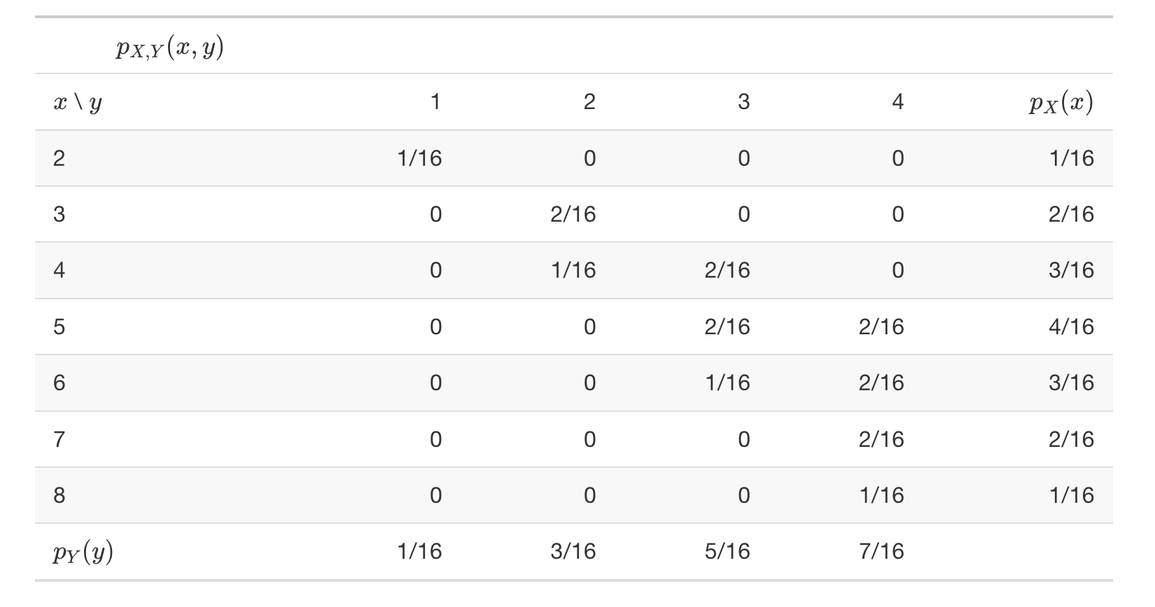
- This is not one "conditional distribution of $Y$ given $X$", but rather a family of conditional distributions of $Y$ given different values of $X$. - Be sure to distinguish between joint, conditional, and marginal distributions. + The **joint** distribution is a distribution on $(X, Y)$ pairs. A mathematical expression of a joint distribution is a function of both values of $X$ and values of $Y$ . In particular, a joint pdf $f_{X, Y}$ is a function of both values of $X$ and values of $Y$. Pay special attention to the possible values; the possible values of one variable might be restricted by the value of the other. + The **conditional** distribution of $Y$ given $X = x$ is a distribution on $Y$ values (among $(X, Y)$ pairs with a fixed value of $X = x$). A mathematical expression of a conditional distribution will involve both $x$ and $y$, but $x$ is treated like a fixed constant and $y$ is treated as the variable. In particular, a conditional pdf $f_{Y|X}$ is a function of values of $Y$ for a fixed value of $x$, treat $x$ like a constant and $y$ as the variable. **Note**: the possible values of $Y$ might depend on the value of $x$, but $x$ is treated like a constant. + The **marginal** distribution of $Y$ is a distribution on $Y$ values only, regardless of the value of $X$. A mathematical expression of a marginal distribution will have only values of the single variable in it; for example, an expression for the marginal distribution of $Y$ will only have $y$ in it (no $x$, not even in the possible values). In particular, a marginal pdf $f_Y$ is a function of values of $Y$ only. # Conditional expection Conditioning on the value of a random variable $X$ in general changes the distribution of another random variable $Y$. If a distribution changes, its summary characteristics like expected value and variance can change too. - The **conditional expectation** (a.k.a. **conditional expected value** a.k.a. **conditional mean**), of a random variable $Y$ given the event $\{X = x\}$, defined on a probability space with measure $P$, is a number denoted $\mathbf{E}(Y|X = x)$ representing the probability-weighted average value of $Y$, where the weights are determined by the **conditional distribution** of $Y$ given $X = x$. + $\textbf{Discrete}$ $(X, Y)$ with conditional pmf $p_{Y|X}$: $$ E(Y|X = x) = \sum_{y} y p_{Y|X} (y|x) $$ + $\textbf{Continuous}$ $(X, Y)$ with conditional pdf $f_{Y|X}$: $$ E(Y|X = x) = \int_{-\infty}^{\infty} y f_{Y|X} (y|x) \, dy $$ ## Conditional expectation as a random variable - Given a value $x$ of $X$, the conditional expected value $\mathbf{E}( Y | X = x)$ is a number. However, since $X$ can take different values $x$, then $\mathbf{E}(Y | X = x)$ can also take different values depending on the value of $x$. - That is, $\mathbf{E}( Y | X = x)$ is a function of $x$. - Since $X$ is a random variable, $\mathbf{E}( Y | X = x)$ is a function of values of a random variable. - The \textit{conditional expectation of $Y$ given $X$} is a \textit{random variable}, denoted as $\textbf{E}(Y|X)$, which takes value $\textbf{E}(Y|X = x)$ on the occurrence of the event $\{X = x\}$. The random variable $\textbf{E}(Y|X)$ is a function of $X$. - Since $\mathbf{E}( Y | X = x)$ is a random variable, it has a distribution. - And since $\mathbf{E}( Y | X = x)$ is a function of $X$, its distribution will depend on the distribution of $X$. However, remember that a transformation generally changes the shape of a distribution, so the distribution of $\mathbf{E}( Y | X = x)$ will usually have a different shape than that of $X$. ## Linearity of conditional expected value - Conditional expected value, whether viewed as a number $\mathbf{E}( Y | X = x)$ or as a random variable $\mathbf{E}(Y|X)$, possesses properties analogous to those of (unconditional) expected value. In particular, we have linearity of conditional expected value. \begin{align*} \mathbf{E}(a_1Y_1 + \ldots + a_nY_n | X = x) & = a_1\mathbf{E}(Y_1 | X = x) + \ldots + a_nE(Y_n | X = x)\\ \mathbf{E}(a_1Y_1 + \ldots + a_nY_n | X) & = a_1\mathbf{E}(Y_1 | X = x) + \ldots + a_nE(Y_n | X) \end{align*} The first line above is an equality involving numbers; the second line is an equality involving random variables (i.e., functions). ## Law of total expectation - The law of total expectation provides a way of computing an expected value by breaking down a problem into various cases, computing the conditional expected value given each case, and then computing the overall expected value as a probability-weighted average of these case-by-case conditional expected values. - **Law of Total Expectation (LTE)** For any two random variables $X$ and $Y$ defined on the same probability space, $$ \mathbf{E}(Y) = \mathbf{E}(\mathbf{E}(Y|X)). $$ + $\mathbf{E}( Y | X = x)$ is a random variable and so it has an expected value $\mathbf{E}(\mathbf{E}(Y|X))$ representing the average value of the random variable $\mathbf{E}(\mathbf{E}(Y|X))$. + $\mathbf{E}( Y | X = x)$ is a function of $X$ and so $\mathbf{E}(\mathbf{E}(Y|X))$ can be computed with respect to $X$. For two discrete random variables X and Y \begin{align*} \mathbf{E}(\mathbf{E}(Y|X)) & = \sum_{x} \mathbf{E}(Y|X = x) \mathbf{P}(X = x)\\ & = \sum_{x} \sum_{y} y \mathbf{P}_{Y|X} (y|x) \mathbf{P}(X = x)\\ & = \sum_{x} \sum_{y} y \mathbf{P}_{X,Y} (x, y)\\ & = \sum_{y} y\sum_{x} \mathbf{P}_{X,Y} (x, y)\\ & = \sum_{y} y \mathbf{P}_{Y} (y)\\ & = \mathbf{E}(Y) \end{align*} # Excercises Roll a fair four-sided die twice. Let $X$ be the sum of the two rolls, and let $Y$ be the larger of the two rolls (or the common value if a tie). We found the joint and marginal distributions of $X$ and $Y$ displayed in the table below.