---
title: "Classification (ISL 4)"
subtitle: "Biostat 212A"
author: "Dr. Jin Zhou @ UCLA"
date: today
format:
  html:
    theme: cosmo
    embed-resources: true
    number-sections: true
    toc: true
    toc-depth: 4
    toc-location: left
    code-fold: false
engine: knitr
knitr:
  opts_chunk: 
    fig.align: 'center'
    # fig.width: 6
    # fig.height: 4
    message: FALSE
    cache: false
---

Credit: This note heavily uses material from the books [_An Introduction to Statistical Learning: with Applications in R_](https://www.statlearning.com/) (ISL2) and [_Elements of Statistical Learning: Data Mining, Inference, and Prediction_](https://hastie.su.domains/ElemStatLearn/) (ESL2).

Display system information for reproducibility.

::: {.panel-tabset}


## R

```{r}
sessionInfo()
```

## Python

```{python}
import IPython
print(IPython.sys_info())
```


:::

## Overview of classification

- Qualitative variables take values in an unordered set $\mathcal{C}$,
such as: $\text{eye color} \in \{\text{brown}, \text{blue}, \text{green}\}$. 

- Given a feature vector $X$ and a qualitative response $Y$
taking values in the set $\mathcal{C}$, the classification task is to build
a function $C(X)$ that takes as input the feature vector $X$ and predicts its value for $Y$, i.e. $C(X) \in \mathcal{C}$.

- Often we are more interested in estimating the probabilities that $X$ belongs to each category in $\mathcal{C}$.

## Credit `Default` data

- Response variable: Credit `default` (`yes` or `no`). 

- Predictors:  
    - `balance`: credit card balance. 
    - `income`: income of customer.  
    - `student`: customer is a student or not.

::: {.panel-tabset}

#### R

```{r}
library(ISLR2)
library(GGally) # ggpairs function
library(tidyverse)
library(pROC)

# Credit default data
Default <- as_tibble(Default) %>% 
  print(width = Inf)

# Visualization by pair plot
ggpairs(
  data = Default, 
  mapping = aes(), 
  lower = list(continuous = "smooth", combo = "box", discrete = "ratio")
  ) + 
  labs(title = "Credit Default Data")
```

```{r}
ggplot(
  data = Default, 
  mapping = aes(x = balance, y = income, color = default)
  ) + 
  geom_point() + 
  labs(
    title = "Credit Default Data", 
    x = "Balance", 
    y = "Income"
    )
```
```{r}
# Visualize income ~ balance
ggplot(
  data = Default, 
  mapping = aes(x = balance, y = income, color = default)
  ) + 
  geom_point() + 
  labs(
    title = "Credit Default Data", 
    x = "Balance", 
    y = "Income"
    )
```

```{r}
# Visualize balance ~ default
ggplot(
  data = Default, 
  mapping = aes(x = default, y = balance)
  ) + 
  geom_boxplot() + 
  labs(
    title = "Credit Default Data", 
    x = "Default", 
    y = "Balance"
    )
```

```{r}
# Visualize income ~ default
ggplot(
  data = Default, 
  mapping = aes(x = default, y = income)
  ) + 
  geom_boxplot() + 
  labs(
    title = "Credit Default Data", 
    x = "Default", 
    y = "Income"
    )
```

```{r}
# Visualize student ~ default
ggplot(
  data = Default, 
  mapping = aes(x = default, fill = student)
  ) + 
  geom_bar(position = "fill") + 
  labs(
    title = "Credit Default Data", 
    x = "Default", 
    y = "Count"
    )
```

#### Python

```{python}
# Load the pandas library
import pandas as pd
# Load numpy for array manipulation
import numpy as np
# Load seaborn plotting library
import seaborn as sns
import matplotlib.pyplot as plt

# Set font sizes in plots
sns.set(font_scale = 1.2)
# Display all columns
pd.set_option('display.max_columns', None)

# Import Credit Default data
Default = pd.read_csv("../data/Default.csv")
Default
```

```{python}
# Visualize income ~ balance
plt.figure()
sns.relplot(
  data = Default, 
  x = 'balance', 
  y = 'income', 
  hue = 'default', 
  style = 'default', 
  height = 10
  ).set(
  xlabel = 'Balance', 
  ylabel = 'Income'
  );
plt.show()  
```

```{python}
# Visualize balance ~ default
plt.figure()
sns.boxplot(
  data = Default, 
  x = 'default', 
  y = 'balance'
  ).set(
  xlabel = 'Default', 
  ylabel = 'Balance'
  );
plt.show()  
```

```{python}
# Visualize income ~ default
plt.figure()
sns.boxplot(
  data = Default, 
  x = 'default', 
  y = 'income'
  ).set(
  xlabel = 'Default', 
  ylabel = 'Income'
  );
plt.show()  
```

```{python}
# Visualize student ~ default
plt.figure()
sns.countplot(
  data = Default, 
  x = 'default', 
  hue = 'student'
  ).set(
  xlabel = 'Default', 
  ylabel = 'Count'
  );
plt.show()  
```

::: 

## Linear vs logistic regression

- If we code `default` as
$$
Y = \begin{cases}
0 & \text{if No} \\
1 & \text{if Yes}
\end{cases},
$$
can we simply perform a linear regression of $Y$ on $X$ and classify as `Yes` if $\hat Y > 0.5$? 

    - Since $\operatorname{E}(Y \mid X = x) = \operatorname{Pr}(Y=1 \mid X = x)$, we might think that linear regression is perfect for this task.  
    
    - The issue is that linear regression may produce probabilities <0 or >1, which does not make sense. 
    
::: {.panel-tabset}

#### R

```{r}
#| label: fig-default-lm-vs-logisitc
#| fig-cap: "Predicted probabilities by linear regression (blue line) vs logistic regression (green line)."
#| code-fold: true

Default %>%
  mutate(y = as.integer(default == "Yes")) %>%
  ggplot(mapping = aes(x = balance, y = y)) + 
  geom_point() + 
  geom_smooth(
    method = "lm",
    color = "blue",
    show.legend = TRUE
    ) + 
  geom_smooth(
    method = "glm", 
    method.args = list(family = binomial),
    color = "green",
    show.legend = TRUE
    ) +
  labs(
    x = "Balance",
    y = "Probability of Default"
    )
```

#### Python

```{python}


# 0-1 (No-Yes) coding
Default['y'] = (Default['default'] == 'Yes').astype(int)
# Linear regression fit vs logistic regression fit
plt.figure()
sns.regplot(
  data = Default, 
  x = 'balance', 
  y = 'y',
  label = 'Linear regression'
  )
sns.regplot(
  data = Default, 
  x = 'balance', 
  y = 'y', 
  logistic = True, 
  label = 'Logistic regression',
  line_kws = {'color': 'g'}
  ).set(
    xlabel = 'Balance', 
    ylabel = 'Probability of Default'
  )
plt.show()  
```

:::

- Now suppose we have a response variable with three possible values. A patient presents at the emergency room, and we must classify them according to their symptoms.
$$
Y = \begin{cases}
1 & \text{if stroke} \\
2 & \text{if drug overdose} \\
3 & \text{if epileptic seizure}
\end{cases}.
$$
This coding suggests an ordering, and in fact implies that the difference between `stroke` and `drug overdose` is the same as between `drug overdose` and `epileptic seizure`. 

    Linear regression is not appropriate here. Multiclass Logistic Regression or Discriminant Analysis are more appropriate.
    
## Logistic regression

- Let's write
$$
p(X) = \operatorname{Pr}(Y = 1 \mid X)
$$
for short. Logistic regression assumes
$$
p(X) = \frac{e^{\beta_0 + \beta_1 X_1 + \cdots + \beta_p X_p}}{1 + e^{\beta_0 + \beta_1 X_1 + \cdots + \beta_p X_p}}.
$$
$p(X) \in [0, 1]$, no matter what values of $\beta_j$ and $X$ take.

- A bit of rearrangement gives
$$
\log \left( \frac{p(X)}{1 - p(X)} \right) = \beta_0 + \beta_1 X_1 + \cdots + \beta_p X_p.
$$
This monotone transformation is called the **log odds** or **logit** transformation of $p(X)$. 

    - The left-hand side is called the **logit** of $p(X)$.
    - The quantity $p(X)/[1−p(X)]$ is called the **odds**, and can take on any value between $[0, \infty]$.
    - For example, on average 1 in 5 people with an odds of $1/4$ will default, since $p(X) = 0.2$ implies an odds of $0.2 = 1/4$.


- We use maximum likelihood to estimate the parameters. That is find $\beta_0, \ldots, \beta_p$ that maximizes the *likelihood* function
$$
\ell(\beta_0, \ldots, \beta_p) = \prod_{i:y_i=1} p(x_i) \prod_{i: y_i = 0} [1 - p(x_i)].
$$

### Optimization for logistic regression (how we actually fit it)

**Model**

- Linear score: $\eta_i = x_i^\top \beta$

- Probability: $p_i = g^{-1}(\eta_i) = \dfrac{1}{1+e^{-\eta_i}}$

**Loss / objective (cross-entropy = negative log-likelihood)**
$$
\mathcal{L}(\beta)
= -\sum_{i=1}^n \Big[ y_i \log(p_i) + (1-y_i)\log(1-p_i) \Big]
$$

- Unlike OLS, minimizing $\mathcal{L}(\beta)$ has **no closed-form solution** → we use iterative optimization.

**Gradient + Hessian (what the optimizer uses)**
Let $p=(p_1,\dots,p_n)^\top$.
$$
\nabla \mathcal{L}(\beta) = X^\top(p - y)
$$
$$
\nabla^2 \mathcal{L}(\beta) = X^\top W X,\quad
W=\mathrm{diag}\big(p_i(1-p_i)\big)
$$

- $\mathcal{L}(\beta)$ is convex ⇒ unique global minimum (when not separable).

**Newton / IRLS update (most common in practice)**
Newton step:
$$
\beta^{(t+1)} = \beta^{(t)} - \left(X^\top W X\right)^{-1} X^\top(p-y)
$$
Equivalent **IRLS** (Iteratively Reweighted Least Squares) view:
1. Compute $p^{(t)}=\sigma(X\beta^{(t)})$ and $W^{(t)}=\mathrm{diag}(p_i^{(t)}(1-p_i^{(t)}))$
2. Form the “working response”
   $$
   z^{(t)} = X\beta^{(t)} + \left(W^{(t)}\right)^{-1}(y - p^{(t)})
   $$
3. Solve weighted least squares
  $$
   \beta^{(t+1)} = \arg\min_\beta \ \| W^{(t)1/2}(z^{(t)} - X\beta)\|_2^2
   $$
4. Repeat until convergence (e.g., change in $\beta$ or $\mathcal{L}(\beta)$ is tiny)

**Practical notes**

- If classes are (quasi-)separable, coefficients can blow up → use regularization (e.g., ridge / lasso) or priors.

- With regularization (ridge):
  $$
  \min_\beta \ \mathcal{L}(\beta) + \lambda\|\beta\|_2^2
  $$
  (same iterative idea, slightly modified updates)


::: {.panel-tabset}

#### R

```{r}
library(gtsummary)

logit_mod <- glm(
  default ~ balance + income + student, 
  family = binomial, 
  data = Default
  )
summary(logit_mod)
```

```{r}
 logit_mod %>% tbl_regression(exponentiate = TRUE)
```


```{r}
# Predicted labels from logistic regression
logit_pred = ifelse(
  predict(logit_mod, Default, type = "response") > 0.5,
  "Yes",
  "No"
)

# Confusion matrix
logit_cfm = table(Predicted = logit_pred, Default = Default$default)

# Accuracy
(logit_cfm['Yes', 'Yes'] + logit_cfm['No', 'No']) / sum(logit_cfm)
```


#### Python (sklearn)

```{python}
from sklearn.linear_model import LogisticRegression
from sklearn.preprocessing import OneHotEncoder
from sklearn.compose import make_column_transformer
from sklearn.pipeline import Pipeline

# Code student as numerical 0/1
col_tf = make_column_transformer(
  # OHE transformer for categorical variables
  (OneHotEncoder(drop = 'first'), ['student']),
  remainder = 'passthrough'
  )
X = Default[['student', 'balance', 'income']]
y = Default['default']

# Pipeline
pipe_logit = Pipeline(steps = [
  ("col_tf", col_tf),
  ("model", LogisticRegression())
])

# Fit logistic regression
logit_fit = pipe_logit.fit(X, y)
logit_fit

# Predicted labels from logistic regression
logit_pred = logit_fit.predict(X)

# Confusion matrix from the logistic regression
logit_cfm = pd.crosstab(
  logit_pred, 
  y,
  margins = True, 
  rownames = ['Predicted Default Stats'],
  colnames = ['True Default Status']
  )
logit_cfm
```
Overall training accuracy of logistic regression (using 0.5 as threshold) is
```{python}
(logit_cfm.loc['Yes', 'Yes'] + logit_cfm.loc['No', 'No']) / logit_cfm.loc['All', 'All']
```
The area-under-ROC curve (AUC) of logistic regression (sklearn) is
```{python}
from sklearn.metrics import roc_auc_score

logit_auc = roc_auc_score(
  y,
  logit_fit.predict_proba(X)[:, 1]
)
logit_auc
```

#### Python (statsmodels)

```{python}
import statsmodels.api as sm
import statsmodels.formula.api as smf

# Fit logistic regression
logit_mod = smf.logit(
  formula = 'y ~ balance + income + student', 
  data = Default
  ).fit()
logit_mod.summary()

# Predicted labels from logistic regression
logit_smpred = np.where(logit_mod.predict(X) > 0.5, 'Yes', 'No')
  
# Confusion matrix from the logistic regression
logit_smcfm = pd.crosstab(
  logit_smpred, 
  y,
  margins = True, 
  rownames = ['Predicted Default Stats'],
  colnames = ['True Default Status']
  )
```

Overall accuracy of logistic regression (by statsmodels)
```{python}
(logit_smcfm.loc['Yes', 'Yes'] + logit_smcfm.loc['No', 'No']) / logit_smcfm.loc['All', 'All']
```

The area-under-ROC curve (AUC) of logistic regression (statsmodels) is
```{python}
logit_smauc = roc_auc_score(
  y,
  logit_mod.predict(X)
)
logit_smauc
```


:::

- We interpret the logistic regression coefficient as the **expected change in log odds** associated with one-unit increase in the corresponding predictor.

    +  Equivalently, it multiplies the odds by a factor of $e^{\beta}$.

- We can measure the accuracy of the coefficient estimates by computing their standard errors. 

- The z-statistic (`z value`) in R output plays the same role as the t-statistic in the linear regression output

    + It is the coefficient divided by its standard error.
    + The null hypotheses is that the coefficient is zero, or equivalently that the **odds ratio** is 1.
    + If pvalue is small, we can reject the null hypothesis and conclude that higher `balance` is associated with the higher probability of `default`.

- Wait! Why the coefficient of `student` is negative, contradicting with the plot?

- **Confounding:** `student` status is confounded with `balance`. Students tend to have higher balances than non-students, so their marginal default rate is higher than for non-students. 
    
    But for each level of balance, students default less than non-students.
    
    Multiple logistic regression can tease this out.
    
::: {.panel-tabset}

#### R
::: {#fig-default-confounding}

```{r}
#| code-fold: true

ggplot(data = Default) + 
  geom_boxplot(mapping = aes(x = student, y = balance)) + 
  labs(
    x = "Student Status",
    y = "Credit Card Balance",
    title = "Students tend to carry larger credit card balance."
    )

Default %>%
  mutate(yhat = logit_mod$fitted.values) %>%
  ggplot() + 
    geom_point(mapping = aes(x = balance, y = yhat, color = student)) +
    labs(
      x = "Credit Card Balance",
      y = "Default Rate",
      subtitle = "Even though students default less at than non-students for each level of balance, marginally their default rate is higher than for non-students."
    )
```
Student status confounds with credit card balance. Students tend to have higher balances than non-students. Even though students default less at than non-students for each level of balance, marginally their default rate is higher than for non-students.

:::

#### Python

```{python}
#| code-fold: true

# Visualize balance ~ default
plt.figure()
sns.boxplot(
  data = Default, 
  x = 'student', 
  y = 'balance'
  ).set(
  xlabel = 'Student Status', 
  ylabel = 'Credit Card Balance'
  );
plt.show()  
```

```{python}
#| code-fold: true

# Add predicted probabilities to DataFrame
Default['yhat'] = logit_mod.predict()
# Visualize yhat ~ balance
plt.figure()
sns.relplot(
  data = Default,
  x = 'balance',
  y = 'yhat',
  kind = 'line',
  hue = 'student',
  height = 8
).set(
  xlabel = 'Credit Card Balance',
  ylabel = 'Default Rate'
);
plt.show()
```


:::

### Making Predictions
- After fitting the logistic regression, for an individual $i$, we can compute the probability of `default` using the estimated coefficients:
$$
\log \left( \frac{ \hat p(\text{balance}_i, \text{income}_i, \text{student}_i)}{1- \hat p(\text{balance}_i, \text{income}_i, \text{student}_i)} \right) = \hat \beta_0 +  \hat \beta_1 \text{balance}_i +  \hat\beta_2 \text{income}_i +\hat \beta_3 \text{student}_i
$$
which is 
$$
\hat p(\text{default}_i = \text{Yes}\mid \text{balance}_i, \text{income}_i, \text{student}_i) = \frac{e^{\hat \beta_0 +  \hat \beta_1 \text{balance}_i +  \hat\beta_2 \text{income}_i + \hat\beta_3 \text{student}_i}}{1+e^{\hat \beta_0 +  \hat \beta_1 \text{balance}_i +  \hat\beta_2 \text{income}_i + \hat\beta_3 \text{student}_i}}
$$
then classify the individual to `default` if $\hat p(\text{balance}_i, \text{income}_i, \text{student}_i) > 0.5$.

- Dummy variable approach is used for qualitative predictors with the logistic regression model as well. 

    + For example, `student` is a qualitative predictor with two levels, `Yes` and `No`. 
    + We can create a dummy variable: a value of $1$ for students and $0$ for non-students. 
    + Then we include this dummy variable as a predictor in the logistic regression equation in order to predict the probability of default for a given value of `balance` for both students and non-students, e.g., a student with a credit card balance of $\$1,500$ and an income of $\$40,000$ has an estimated probability of `default` of
\begin{eqnarray*}
& & \hat p(\text{default = Yes} | \text{balance = 1500, income = 40,000, student = Yes})  \\
&=& \frac{e^{−10.869+0.00574\times 1500+0.003\times 40−0.6468\times 1}}{1 + e^{−10.869+0.00574\times 1500+0.003\times40−0.6468\times 1}} \\
&=& 0.058
\end{eqnarray*}

- We can use the `predict()` function to predict the probability that a given observation belongs to a particular class, rather than predicting the class itself.
```{r}
(p = predict(logit_mod, 
             newdata = data.frame(balance = 1500, income = 40000, student = "Yes"), 
             type = "response"))
```

## Multinomial logit regression

For more than two classes, we generalize logistic regression to
$$
\operatorname{Pr}(Y = k \mid X) = \frac{e^{\beta_{0k} + \beta_{1k} X_1 + \cdots + \beta_{pk} X_p}}{\sum_{\ell = 1}^K e^{\beta_{0\ell} + \beta_{1\ell} X_1 + \cdots + \beta_{p\ell} X_p}}.
$$
Note each class has its own set of regression coefficients.

- We first select a single class to serve as the baseline; then for each of the remaining $K-1$ classes, we fit a separate binary logistic regression model that compares that class to the baseline.
$$
p(Y=k|X=x) = \frac{e^{\beta_{k0}+\beta_{k1}x_1+\ldots+\beta_{kp}x_p}}{1+\sum_{\ell=1}^{K-1}e^{\beta_{\ell0}+\beta_{\ell1}x_1+\ldots+\beta_{\ell p}x_p}}, \quad k=1,\ldots,K-1.
$$
and the baseline class is
$$
p(Y=K|X=x) = \frac{1}{1+\sum_{\ell=1}^{K-1}e^{\beta_{\ell0}+\beta_{\ell1}x_1+\ldots+\beta_{\ell p}x_p}}.
$$
Then we can show
$$
\log\left(\frac{p(Y=k|X=x)}{p(Y=K|X=x)}\right) = \beta_{k0}+\beta_{k1}x_1+\ldots+\beta_{kp}x_p, \quad k=1,\ldots,K-1.
$$
- Therefore, the interpretation of the coefficients in a multinomial logistic regression model is tied to the choice of baseline.
    + For example, if we set  `epileptic seizure` to be the baseline, then a one-unit increase in $X_j$ is associated with a $\beta_{stroke,j}$ increase in the log odds of stroke over epileptic seizure. Stated another way, if $X_j$ increases by one unit, then the odds of stroke over epileptic seizure 
$$
\frac{p(Y=\text{stroke}|X=x)}{p(Y=\text{epileptic seizure}|X=x)}
$$
are multiplied by $e^{\beta_{stroke,j}}$.

In Python, we can fit multinomial logit model by [`statsmodels.discrete.discrete_model.MNLogit`](https://www.statsmodels.org/dev/generated/statsmodels.discrete.discrete_model.MNLogit.html). In R, we can use `glmnet` package or `nnet` package.

## Discriminant analysis

- Another approach for classification is to model the distribution of $X$ in each of the classes separately, and then use **Bayes theorem** to flip things around and obtain $\operatorname{Pr}(Y = j \mid X)$.

- When we use normal (Gaussian) distributions for each class, this leads to linear or quadratic discriminant analysis.

- However, this approach is quite general, and other distributions can be used as well. We will focus on normal distributions.

- [Thomas Bayes](https://en.wikipedia.org/wiki/Thomas_Bayes) was a famous mathematician whose name represents a big subfield of statistical and probabilistic modeling. Here we focus on a simple result, known as **Bayes theorem**:
\begin{eqnarray*}
p_k(x) &=& \operatorname{Pr}(Y = k \mid X = x) \\
&=& \frac{\operatorname{Pr}(X = x, Y = k)}{\operatorname{Pr}(X = x)} \\
&=& \frac{\operatorname{Pr}(X = x \mid Y = k) \cdot \operatorname{Pr}(Y = k)}{\operatorname{Pr}(X = x)} \\
&=& \frac{\pi_k f_k(x)}{\sum_{\ell=1}^K \pi_\ell f_\ell(x)},
\end{eqnarray*}
where   
    - $f_k(x) = \operatorname{Pr}(X = x \mid Y = k)$ is the density of $X$ in class $k$  
    - $\pi_k = \operatorname{Pr}(Y = k)$ is the marginal or **prior** probability for class $k$. 
    
- Advantages of discriminant analysis.

    - When the classes are well-separated, the parameter estimates for the logistic regression model are surprisingly unstable (separation or quasi-separation). Linear discriminant analysis does not suffer from this problem.
    
    - If $n$ is small and the distribution of the predictors $X$ is approximately normal in each of the classes, the linear discriminant model is again more stable than the logistic regression model.
    
### Linear discriminant analysis (LDA)
    
- Assume $X \in \mathbb{R}^p$ in the $k$-th class is distributed as as multivariate normal $N(\mu_k, \boldsymbol{\Sigma})$ with density
$$
f_k(x) = \frac{1}{(2\pi)^{p/2} |\boldsymbol{\Sigma}|^{1/2}} e^{- \frac{1}{2} (x - \mu_k)^T \boldsymbol{\Sigma}^{-1} (x - \mu_k)}.
$$
To classify $X=x$, we need to see which of $p_k(x)$ is big. Taking logs, and discarding terms that do not depend on $k$, we just need to assign $x$ to the class with the largest **discriminant score**
$$
\delta_k(x) = x^T \boldsymbol{\Sigma}^{-1} \mu_k - \frac{1}{2} \mu_k^T \boldsymbol{\Sigma}^{-1} \mu_k + \log \pi_k,
$$
which is a linear function in $x$!

    + For example, in the one-dimensional setting, the normal density takes the form
$$
f_k(x) = \frac{1}{\sqrt{2\pi\sigma_k}} \exp\left(-\frac{1}{2\sigma_k^2}(x - \mu_k)^2\right)
$$
    + where $\mu_k$ and $\sigma_{k}^2$ are the mean and variance parameters for the $k$th class. We assume shared variance term across all $K$ classes, $\sigma_{1}^2=\ldots=\sigma_{K}^2 = \sigma^2$. Then 
$$
p_k(x) = \frac{\pi_k \frac{1}{\sqrt{2\pi\sigma}} \exp\left(-\frac{1}{2\sigma^2}(x - \mu_k)^2\right)}{\sum_{l=1}^{K} \pi_l \frac{1}{\sqrt{2\pi\sigma}} \exp\left(-\frac{1}{2\sigma^2}(x - \mu_l)^2\right)}.
$$
      Taking the log of both sides and rearrange terms with $k$
$$
\delta_k = x \frac{\mu_k}{\sigma^2} - \frac{\mu_k^2}{2\sigma^2} + \log \pi_k.
$$ 

- The linear discriminant function $\delta_k(x)$ is a linear combination of the features $x_1, \ldots, x_p$.

- We estimate the unknown parameters $\pi_k$, $\mu_k$, and $\boldsymbol{\Sigma}$ by
\begin{eqnarray*}
\hat{\pi}_k &=& \frac{n_k}{n} \\
\hat{\mu}_k &=& \frac{1}{n_k} \sum_{i: y_i = k} x_i \\
\hat{\boldsymbol{\Sigma}} &=& \frac{1}{n-K} \sum_{k=1}^K \sum_{i: y_i = k} (x_i - \hat \mu_k)(x_i - \hat \mu_k)^T.
\end{eqnarray*}

- Once we have estimated $\hat \delta_k(x)$, we can turn these into class probabilities
$$
\hat{\operatorname{Pr}}(Y = k \mid X = x) = \frac{e^{\hat \delta_k(x)}}{\sum_{\ell=1}^K e^{\hat \delta_{\ell}(x)}}.
$$

::: {#fig-tradeoff-truth}

<p align="center">
![](ISL_fig_4_6.pdf){width=700px height=350px}
</p>

Here $\pi_1 = \pi_2 = \pi_3 = 1/3$. The dashed lines are known as the Bayes decision boundaries. Were they known, they would yield the fewest misclassification errors, among all possible classifiers. The black line is the LDA decision boundary.

:::

- LDA on the credit `Default` data.

::: {.panel-tabset}


#### R

```{r}
library(MASS)

# Fit LDA
lda_mod <- lda(
  default ~ balance + income + student, 
  data = Default
  )
lda_mod

# Predicted labels from LDA
lda_pred = predict(lda_mod, Default)

# Confusion matrix
(lda_cfm = table(Predicted = lda_pred$class, Default = Default$default))

```

Overall training accuracy of LDA (using 0.5 as threshold) is
```{r}
# Accuracy
(lda_cfm['Yes', 'Yes'] + lda_cfm['No', 'No']) / sum(lda_cfm)
```

The area-under-ROC curve (AUC) of LDA is
```{r}
# AUC

(lda_auc = roc(Default$default, lda_pred$posterior[, 2])$auc)
```

#### Python

```{python}
from sklearn.discriminant_analysis import LinearDiscriminantAnalysis

# Pipeline
pipe_lda = Pipeline(steps = [
  ("col_tf", col_tf),
  ("model", LinearDiscriminantAnalysis())
])

# Fit LDA
lda_fit = pipe_lda.fit(X, y)

# Predicted labels from LDA
lda_pred = lda_fit.predict(X)

# Confusion matrix
lda_cfm = pd.crosstab(
  lda_pred, 
  y, 
  margins = True, 
  rownames = ['Predicted Default Stats'],
  colnames = ['True Default Status']
  )
lda_cfm
```
:::


The area-under-ROC curve (AUC) of LDA is
```{python}
lda_auc = roc_auc_score(
  y,
  lda_fit.predict_proba(X)[:, 1]
)
lda_auc
```


- Note: 

    + Training error rates will usually be lower than test error rates, which are the real quantity of interest. 
    + The higher the ratio of parameters $p$ to number of samples n, the more we expect this overfitting to play a role.
    + Since only $3.33\%$ of the individuals in the training sample defaulted, a simple but useless classifier that always predicts that an individual will not default, regardless of his or her credit card balance and student status, will result in an error rate of $3.33\%$. In other words, the trivial **null classifier** will achieve an error rate that null is only a bit higher than the LDA training set error rate.

- However this can change, depending how we define `default`. In the two-class case, we often assign an observation to the `default` class if
$$
p(\text{default = Yes}|X = x) > 0.5
$$

- But if we are interested in minimizing the number of defaults that we fail to identify, then we should instead assign an observation to the `default` class if
$$
p(\text{default = Yes}|X = x) > 0.2.
$$

### Quadratic discriminant analysis (QDA)

- In LDA, the normal distribution for each class shares the same covariance $\boldsymbol{\Sigma}$.

- If we assume that the normal distribution for class $k$ has covariance $\boldsymbol{\Sigma}_k$, then it leads to the **quadratic discriminant analysis** (QDA).

- The discriminant function takes the form
$$
\delta_k(x) = - \frac{1}{2} (x - \mu_k)^T \boldsymbol{\Sigma}_k^{-1} (x - \mu_k) + \log \pi_k - \frac{1}{2} \log |\boldsymbol{\Sigma}_k|,
$$
which is a quadratic function in $x$.

::: {#fig-lda-vs-qda}

<p align="center">
![](ISL_fig_4_9.pdf){width=700px height=350px}
</p>

The Bayes (purple dashed), LDA (black dotted), and QDA (green solid) decision boundaries for a two-class problem. Left: $\boldsymbol{\Sigma}_1 = \boldsymbol{\Sigma}_2$. Right: $\boldsymbol{\Sigma}_1 \ne \boldsymbol{\Sigma}_2$.

:::

::: {.panel-tabset}

#### R

```{r}
# Fit QDA
qda_mod <- qda(
  default ~ balance + income + student, 
  data = Default
  )
qda_mod

# Predicted probabilities from QDA
qda_pred = predict(qda_mod, Default)

# Confusion matrix
(qda_cfm = table(Predicted = qda_pred$class, Default = Default$default))
```

Overall training accuracy of QDA (using 0.5 as threshold) is
```{r}
# Accuracy
(qda_cfm['Yes', 'Yes'] + qda_cfm['No', 'No']) / sum(qda_cfm)
```

The area-under-ROC curve (AUC) of QDA is
```{r}
(auc_qda = roc(
  Default$default,
  qda_pred$posterior[, 'Yes']
)$auc)
```

#### Python

```{python}
from sklearn.discriminant_analysis import QuadraticDiscriminantAnalysis

# Pipeline
pipe_qda = Pipeline(steps = [
  ("col_tf", col_tf),
  ("model", QuadraticDiscriminantAnalysis())
])

# Fit QDA
qda_fit = pipe_qda.fit(X, y)

# Predicted labels from QDA
qda_pred = qda_fit.predict(X)

# Confusion matrix from the QDA
qda_cfm = pd.crosstab(
  qda_pred, 
  y,
  margins = True, 
  rownames = ['Predicted Default Stats'],
  colnames = ['True Default Status']
  )
qda_cfm
```

Overall training accuracy of QDA (using 0.5 as threshold) is
```{python}
(qda_cfm.loc['Yes', 'Yes'] + qda_cfm.loc['No', 'No']) / qda_cfm.loc['All', 'All']
```

The area-under-ROC curve (AUC) of QDA is
```{python}
qda_auc = roc_auc_score(
  y,
  qda_fit.predict_proba(X)[:, 1]
)
qda_auc
```

:::

### Naive Bayes

- If we assume $f_k(x) = \prod_{j=1}^p f_{jk}(x_j)$ (conditional independence model) in each class, we get **naive Bayes**. 

    For Gaussian this means the $\boldsymbol{\Sigma}_k$ are diagonal.

- Naive Bayes is useful when $p$ is large (LDA and QDA break down).

- Can be used for $mixed$ feature vectors (both continuous and categorical). If $X_j$ is qualitative, replace $f_{kj}(x_j)$ with probability mass function (histogram) over discrete
categories.

- Despite strong assumptions, naive Bayes often produces good classification results.

::: {.panel-tabset}



#### R
- Note : For each categorical variable a table giving, for each attribute level, the conditional probabilities given the target class. For each numeric variable, a table giving, for each target class, mean and standard deviation of the (sub-)variable.
```{r}
library(e1071)

# Fit Naive Bayes classifier
nb_mod <- naiveBayes(
  default ~ balance + income + student, 
  data = Default
  )
nb_mod

# Predicted labels from Naive Bayes
nb_pred = predict(nb_mod, Default)

# Confusion matrix
(nb_cfm = table(Predicted = nb_pred, Default = Default$default))
```

Overall training accuracy of Naive Bayes classifier (using 0.5 as threshold) is
```{r}
# Accuracy
(nb_cfm['Yes', 'Yes'] + nb_cfm['No', 'No']) / sum(nb_cfm)
```

The area-under-ROC curve (AUC) of NB is
```{r}
(auc_nb = roc(
  Default$default, 
  predict(nb_mod, Default, type = "raw")[, 2]
  )$auc)
```

#### Python

```{python}
from sklearn.naive_bayes import GaussianNB

# Pipeline
pipe_nb = Pipeline(steps = [
  ("col_tf", col_tf),
  ("model", GaussianNB())
])

# Fit Naive Bayes classifier
nb_fit = pipe_nb.fit(X, y)

# Predicted labels by NB classifier
nb_pred = nb_fit.predict(X)

# Confusion matrix of NB classifier
nb_cfm = pd.crosstab(
  nb_pred, 
  y, 
  margins = True, 
  rownames = ['Predicted Default Stats'],
  colnames = ['True Default Status']
  )
nb_cfm
```

Overall training accuracy of Naive Bayes classifier (using 0.5 as threshold) is
```{python}
(nb_cfm.loc['Yes', 'Yes'] + nb_cfm.loc['No', 'No']) / nb_cfm.loc['All', 'All']
```

The area-under-ROC curve (AUC) of NB is
```{python}
nb_auc = roc_auc_score(
  y,
  nb_fit.predict_proba(X)[:, 1]
)
nb_auc
```

:::

## $K$-nearest neighbor (KNN) classifier

- KNN is a nonparametric classifier. 

- Given a positive integer $K$ and a test observation $x_0$, the KNN classifier first identifies the $K$ points in the training data that are closest to $x_0$, represented by $\mathcal{N}_0$. It estimates the conditional probability by
$$
\operatorname{Pr}(Y=j \mid X = x_0) = \frac{1}{K} \sum_{i \in \mathcal{N}_0} I(y_i = j)
$$
and then classifies the test observation $x_0$ to the class with the largest probability.

- We illustrate KNN with $K=5$ on the credit default data.

::: {.panel-tabset}

#### R

```{r}
library(class)

X_default <- Default %>% 
  mutate(x_student = as.integer(student == "Yes")) %>%
  dplyr::select(x_student, balance, income)

# KNN prediction with K = 5
knn_pred <- knn(
  train = X_default, 
  test = X_default,
  cl = Default$default,
  k = 5
  )

# Confusion matrix
(knn_cfm = table(Predicted = knn_pred, Default = Default$default))
```

Overall training accuracy of KNN classifier with $K=5$ (using 0.5 as threshold) is
```{r}
# Accuracy
(knn_cfm['Yes', 'Yes'] + knn_cfm['No', 'No']) / sum(knn_cfm)
```

The area-under-ROC curve (AUC) of KNN ($K=5$) is
```{r}
# AUC
knn_mod <- knn(
  train = X_default, 
  test = X_default,
  cl = Default$default,
  prob = TRUE,
  k = 5
  )
knn_pred_prob <- 1 - attr(knn_mod, "prob") 

(knn_auc = auc(
  Default$default,
  knn_pred_prob
))
```

#### Python

```{python}
from sklearn.neighbors import KNeighborsClassifier

# Pipeline
pipe_knn = Pipeline(steps = [
  ("col_tf", col_tf),
  ("model", KNeighborsClassifier(n_neighbors = 5))
])

# Fit KNN with K = 5
knn_fit = pipe_knn.fit(X, y)

# Predicted labels from KNN
knn_pred = knn_fit.predict(X)

# Confusion matrix of KNN
knn_cfm = pd.crosstab(
  knn_pred, 
  y, 
  margins = True, 
  rownames = ['Predicted Default Stats'],
  colnames = ['True Default Status']
  )
knn_cfm
```

Overall training accuracy of KNN classifier with $K=5$ (using 0.5 as threshold) is
```{python}
(knn_cfm.loc['Yes', 'Yes'] + knn_cfm.loc['No', 'No']) / knn_cfm.loc['All', 'All']
```

The area-under-ROC curve (AUC) of KNN ($K=5$) is
```{python}
knn_auc = roc_auc_score(
  y,
  knn_fit.predict_proba(X)[:, 1]
)
knn_auc
```
:::

## Evaluation of classification performance: false positive, false negative, ROC and AUC

- Let's summarize the classification performance of different classifiers on the training data. 

::: {.panel-tabset}

#### R
```{r, message=F}
library(pROC)

acc_f = function(cfm) {
  (cfm['Yes', 'Yes'] + cfm['No', 'No']) / sum(cfm)
}

fpr_f = function(cfm) {
  cfm['Yes', 'No'] / sum(cfm[, 'No'])
}

fnr_f = function(cfm) {
  cfm['No', 'Yes'] / sum(cfm[, 'Yes'])
}

auc_f = function(pred) {
  y = pred$y
  pred_prob = pred$prob
  roc_object <- roc(y, pred_prob)
  auc_c = auc(roc_object)[1]
  return(auc_c)
}

logit_pred_prob <- predict(logit_mod, Default, type = "response")
lda_pred_prob <- lda_pred$posterior[, 2]
qda_pred_prob <- qda_pred$posterior[, 2]
nb_pred_prob <- predict(nb_mod, Default, type = "raw")[, 2]
knn_mod <- knn(
  train = X_default, 
  test = X_default,
  cl = Default$default,
  prob = TRUE,
  k = 5
  )
knn_pred_prob <- 1 - attr(knn_mod, "prob") 

row_names = c("Null", "Logit", "LDA", "QDA", "NB", "KNN")
acc_v = sapply(list(logit_cfm, lda_cfm, qda_cfm, nb_cfm, knn_cfm), acc_f)
fpr_v = sapply(list(logit_cfm, lda_cfm, qda_cfm, nb_cfm, knn_cfm), fpr_f)
fnr_v = sapply(list(logit_cfm, lda_cfm, qda_cfm, nb_cfm, knn_cfm), fnr_f)
auc_v = sapply(list(data.frame(y = Default$default,
                             prob = logit_pred_prob), 
                  data.frame(y = Default$default,
                             prob = lda_pred_prob), 
                  data.frame(y = Default$default,
                             prob = qda_pred_prob), 
                  data.frame(y = Default$default,
                             prob = nb_pred_prob), 
                  data.frame(y = Default$default,
                             prob = knn_pred_prob)), 
             auc_f)
cfm_null =  matrix(c(9667, 333, 0, 0), nrow = 2, ncol = 2, byrow = TRUE)
row.names(cfm_null) <- c("No", "Yes")
colnames(cfm_null) <- c("No", "Yes")

tibble(Classifier = row_names, 
       ACC = c(acc_f(cfm_null), acc_v), 
       FPR = c(fpr_f(cfm_null), fpr_v), 
       FNR = c(fnr_f(cfm_null), fnr_v), 
       AUC = c(0.5, auc_v))

```

#### Python

```{python}
# Confusion matrix from the null classifier (always 'No')
null_cfm = pd.DataFrame(
  data = {
    'No': [9667, 0, 9667],
    'Yes': [333, 0, 333],
    'All': [10000, 0, 10000]
    },
  index = ['No', 'Yes', 'All']
  )
null_pred = np.repeat('No', 10000)
# Fitted classifiers
classifiers = [logit_fit, lda_fit, qda_fit, nb_fit, knn_fit]
# Confusion matrices
cfms = [logit_cfm, lda_cfm, qda_cfm, nb_cfm, knn_cfm, null_cfm]
```

```{python}
sm_df = pd.DataFrame(
  data = {
  'acc': [(cfm.loc['Yes', 'Yes'] + cfm.loc['No', 'No']) / cfm.loc['All', 'All'] for cfm in cfms],
  'fpr': [(cfm.loc['Yes', 'No'] / cfm.loc['All', 'No']) for cfm in cfms],
  'fnr': [(cfm.loc['No', 'Yes'] / cfm.loc['All', 'Yes']) for cfm in cfms],
  'auc': np.append([roc_auc_score(y, c.predict_proba(X)[:, 1]) for c in classifiers], roc_auc_score(y, np.repeat(0, 10000)))
  },
  index = ['logit', 'LDA', 'QDA', 'NB', 'KNN', 'Null']
  )
sm_df.sort_values('acc')
```

:::

- There are two types of classification errors:

    - **False positive rate**: The fraction of negative examples that are classified as positive.
    - **False negative rate**: The fraction of positive examples that are classified as negative.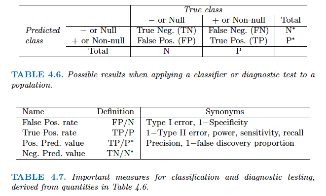
    
![](./classification_measures.png)

- Above table is the training classification performance of classifiers using their default thresholds. Varying thresholds lead to varying false positive rates (1 - specificity) and true positive rates (sensitivity). These can be plotted as the **receiver operating characteristic (ROC)** curve. The overall performance of a classifier is summarized by the **area under ROC curve (AUC)**.

::: {.panel-tabset}

#### R

```{r, message=F}
library(pROC)
classifiers = c("Logit", "LDA", "QDA", "NB", "KNN", "Null")

for(i in seq(1, length(classifiers))) {
# i = 1
  pred = list(
    logit = data.frame(y = Default$default,
                       prob = logit_pred_prob),
    LDA = data.frame(y = Default$default,
                     prob = lda_pred_prob),
    QDA = data.frame(y = Default$default,
                     prob = qda_pred_prob),
    NB = data.frame(y = Default$default,
                    prob = nb_pred_prob),
    KNN = data.frame(y = Default$default,
                     prob = knn_pred_prob),
    Null = data.frame(y = Default$default,
                      prob = rep(0, 10000))
    )
  roc_object <- roc(pred[[i]]$y, pred[[i]]$prob)
  auc_c = auc(roc_object)[1]
  
  print(ggroc(roc_object) + 
    ggtitle(str_c(classifiers[i], " ROC with AUC =", round(auc_c, 4), "")) +
    annotate("segment",x = 1, xend = 0, y = 0, yend = 1, color="red", linetype="dashed") +
    labs(x = "1 - Specificity", y = "Sensitivity"))
}


```

#### Python

```{python}
from sklearn.metrics import roc_curve
from sklearn.metrics import RocCurveDisplay

# plt.rcParams.update({'font.size': 12})
for idx, m in enumerate(classifiers):
  plt.figure();
  RocCurveDisplay.from_estimator(m, X, y, name = sm_df.iloc[idx].name);
  plt.show()
  
# ROC curve of the null classifier (always No or always Yes)  
plt.figure()
RocCurveDisplay.from_predictions(y, np.repeat(0, 10000), pos_label = 'Yes', name = 'Null Classifier');
plt.show()
```

:::

- See [sklearn.metrics](https://scikit-learn.org/stable/modules/model_evaluation.html) for other popularly used metrics for classification tasks.

## Comparison between classifiers

- For a two-class problem, we can show that for LDA,
$$
\log \left( \frac{p_1(x)}{1 - p_1(x)} \right) = \log \left( \frac{p_1(x)}{p_2(x)} \right) = c_0 + c_1 x_1 + \cdots + c_p x_p.
$$
So it has the same form as logistic regression. The difference is in how the parameters are estimated. 

- Logistic regression uses the conditional likelihood based on $\operatorname{Pr}(Y \mid X)$ (known as **discriminative learning**). 

    LDA, QDA, and Naive Bayes use the full likelihood based on $\operatorname{Pr}(X, Y)$ (known as **generative learning**).
    
- Despite these differences, in practice the results are often very similar.

- Logistic regression can also fit quadratic boundaries like QDA, by explicitly including quadratic terms in the model.

- Logistic regression is very popular for classification, especially when $K = 2$.

- LDA is useful when $n$ is small, or the classes are well separated, and Gaussian assumptions are reasonable. Also when $K > 2$.

- Naive Bayes is useful when $p$ is very large.

- LDA is a special case of QDA. 

- Under normal assumption, Naive Bayes leads to linear decision boundary, thus a special case of LDA. 

- KNN classifier is non-parametric and can dominate LDA and logistic regression when the decision boundary is highly nonlinear, provided that $n$ is very large and $p$ is small.

- See ISL Section 4.5 for theoretical and empirical comparisons of logistic regression, LDA, QDA, NB, and KNN.

## Poisson regression
- $Y$ is neither qualitative nor quantitative, but rather a count.
- For example,  `Bikeshare` data set: 
    + The response is `bikers`, the number of hourly users of a bike sharing program in Washington, DC.
    + Predictors: 
        + `mnth` month of the year, 
        + `hr` hour of the day, from 0 to 23, 
        + `workingday` an indicator variable that equals 1 if it is neither a weekend nor a holiday, 
        + `temp` the normalized temperature, in Celsius, 
        + `weathersit` a qualitative variable that takes on one of four possible values: clear; misty or cloudy; light rain or light snow; or heavy rain or heavy snow.
        
```{r}
library(ISLR2)
ggplot(Bikeshare, aes(x = bikers)) + 
  geom_histogram(bins = 40) 
```
### Try linear regression 
```{r}
library(ISLR2)
Bikeshare <- as_tibble(Bikeshare) %>%
  mutate(mnth = factor(mnth),
         hr = factor(hr),
         workingday = factor(workingday, levels = c(0, 1), labels = c("No", "Yes")),
         weathersit = factor(weathersit))
```

```{r, message=F, warning=F}
m1 <- lm(bikers ~ workingday + temp + weathersit, data = Bikeshare)

m1 %>% tbl_regression(
    pvalue_fun = ~ style_pvalue(.x, digits = 2),
    estimate_fun = function(x) style_number(x, digits = 3)
  ) %>%
  add_global_p() %>%
  bold_p(t = 0.05) %>%
  bold_labels() %>%
  modify_column_unhide(columns = c(statistic, std.error)) %>%
  add_glance_source_note(
    label = list(sigma ~ "\U03C3"),
    include = c(r.squared, sigma)) %>%
  add_n(location = "label")
```

::: {.panel-tabset}
#### R
Part of the fitted values in the `Bikeshare` data set are negative.
```{r}
m1 %>% 
  ggplot(aes(x  = .fitted)) +
  geom_histogram() 
```

:::

- Mean-variance relationship 
    + It shows that the smaller the mean, the smaller the variance.
    + This violates the assumption of **constant variance** in linear regression.
```{r}
ggplot(Bikeshare %>% mutate(hr = as.numeric(hr)), 
       aes(x = hr, y = bikers)) +
  geom_point() +
  geom_jitter(width = 0.1) +
  geom_smooth(method = "loess", span = 0.65) 
```
- We could do a transformation, i.e., $\log$
$$
\log(Y) = \sum_{j=1}^p \beta_j X_j + \epsilon.
$$
    + But the model is no longer linear in the predictors and the interpretation of the coefficients is for $\log(Y)$ rather than $Y$.
    
### Poisson regression
- We often use Poisson regression to model counts $Y$.
- Poisson distribution: a random variable $Y$ takes on nonnegative integer values, i.e. $Y \in \{0, 1, 2, \ldots\}$. If $Y$ follows the Poisson distribution, then 
$$
p(Y=k) = \frac{\lambda^k e^{-\lambda}}{k!}, \quad k = 0, 1, 2, \ldots
$$
where $\lambda$ is the **mean and variance** of $Y$, i.e., $\mathbf{E}(Y)$.

- Poisson regression model: 
    + Assume that $Y$ follows a Poisson distribution with mean $\lambda$.
    + We model the log mean as a linear function of the predictors:
$$
\log(\lambda(X_1, \ldots, X_p)) = \beta_0 + \beta_1 X_1 + \cdots + \beta_p X_p.
$$
or equivalently
$$
\lambda(X_1, \ldots, X_p) = \exp(\beta_0 + \beta_1 X_1 + \cdots + \beta_p X_p).
$$

- To estimate the parameters $\beta_0, \ldots, \beta_p$, we use the method of maximum likelihood. 
    + The likelihood function is
$$
\ell(\beta_0,\ldots,\beta_p) = \prod_{i=1}^n \frac{\lambda_i(x_i)^{y_i} e^{-\lambda_i}}{y_i!}
$$
    + We estimate the coefficients that maximize the likelihood $\ell(\beta_0,\ldots,\beta_p)$ i.e. that make the observed data as likely as possible.
    
```{r, message=F, warning=F}
m1 <- glm(bikers ~ workingday + temp + weathersit, data = Bikeshare, family = poisson)

m1 %>% tbl_regression(
    pvalue_fun = ~ style_pvalue(.x, digits = 2),
    estimate_fun = function(x) style_number(x, digits = 3)
  ) %>%
  add_global_p() %>%
  bold_p(t = 0.05) %>%
  bold_labels() %>%
  modify_column_unhide(columns = c(statistic, std.error)) %>%
  add_n(location = "label")
```
- Interpretation: an increase in $X_j$ by one unit is associated with a change in $\mathbf{E}(Y ) = \lambda$ by a factor of $\exp(\beta_j)$.
- Mean-variance relationship: since under the Poisson model, $\lambda = \mathbf{E}(Y ) = \mathbf{Var}(Y)$, we implicitly modeled variance, not a constant any more. If variance is much larger than the mean, i.e., overdispersion, we can use negative binomial regression instead.
- Nonnegative fitted values: no negative predictions using the Poisson regression model. This is because the Poisson model itself assumes that the response is nonnegative.
    
## Generalized linear models

- We have now discussed three types of regression models: linear, logistic, and Poisson. These approaches share some common characteristics:
    + Each approach uses predictors $X_1,\ldots,X_p$ to predict a response $Y$. 
    + We assume that, conditional on $X_1,\ldots,X_p$, $Y$ belongs to a certain family of distributions. 
        + For linear regression, assume that $Y$ follows a Gaussian or normal distribution. 
        + For logistic regression, we assume that $Y$ follows a Bernoulli distribution. 
        + For Poisson regression, we assume that $Y$ follows a Poisson distribution.
    + Each approach models the mean of $Y$ as a function of the predictors. 
        + In linear regression, the mean of $Y$ takes the form, i.e., linear function of the predictors
$$
\mathbf{E}(Y \mid X_1,\ldots,X_p) = \beta_0 + \beta_1 X_1 + \cdots + \beta_p X_p.
$$  
    + For logistic regression, the mean instead takes the form
$$
\mathbf{E}(Y \mid X_1,\ldots,X_p) = \frac{\exp(\beta_0 + \beta_1 X_1 + \cdots + \beta_p X_p)}{1 + \exp(\beta_0 + \beta_1 X_1 + \cdots + \beta_p X_p)}.
$$
    + For Poisson regression, the mean instead takes the form
$$
\mathbf{E}(Y \mid X_1,\ldots,X_p) = \exp(\beta_0 + \beta_1 X_1 + \cdots + \beta_p X_p).
$$
- Each equation can be expressed using a **link function**, $\eta$, which applies a transformation to $\mathbf{E}(Y \mid X_1,\ldots,X_p)$ so that the transformed mean is a linear function of the predictors 
$$
\eta(\mathbf{E}(Y \mid X_1,\ldots,X_p)) = \beta_0 + \beta_1 X_1 + \cdots + \beta_p X_p.
$$
     + The link function for linear regression is the identity function, $\eta(\mu) = \mu$.
     + The link function for logistic regression is the logit function, $\eta(\mu) = \log(\mu/(1-\mu))$.
     + The link function for Poisson regression is the log function, $\eta(\mu) = \log(\mu)$.
- The Gaussian, Bernoulli and Poisson distributions are all members of a wider class of distributions, known as the exponential family.
- In general, we form a regression by modeling the response $Y$ as from a particular member of the exponential family, and then transforming the mean of the response so that the transformed mean is a linear function of the predictors via $\eta(\mathbf{E}(Y \mid X_1,\ldots,X_p)) = \beta_0 + \beta_1 X_1 + \cdots + \beta_p X_p$.
- Any regression approach that follows this very general recipe known as a **generalized linear model(GLM)**. Thus, linear regression, logistic regression, and Poisson regression are all special cases of GLMs.
- Other examples include Gamma regression and negative binomial regression.