{width=500px height=400px}
The population size (`pop`) and ad spending (`ad`) for 100 different cities are shown as purple circles. The green solid line indicates the first principal component, and the blue dashed line indicates the second principal component. ::: ### Computation of PCs - Suppose we have an $n \times p$ data set $\boldsymbol{X}$. Since we are only interested in variance, we assume that each of the variables in $\boldsymbol{X}$ has been centered to have mean zero (that is, the column means of $\boldsymbol{X}$ are zero). - We then look for the linear combination of the sample feature values of the form $$ z_{i1} = \phi_{11} x_{i1} + \phi_{21} x_{i2} + \cdots + \phi_{p1} x_{ip} $$ {#eq-pc-1} for $i=1,\ldots,n$ that has largest sample variance, subject to the constraint that $\sum_{j=1}^p \phi_{j1}^2 = 1$. - Since each of the $x_{ij}$ has mean zero, then so does $z_{i1}$ (for any values of $\phi_{j1}$). Hence the sample variance of the $z_{i1}$ can be written as $\frac{1}{n} \sum_{i=1}^n z_{i1}^2$. - Plugging in (@eq-pc-1) the first principal component loading vector solves the optimization problem $$ \max_{\phi_{11},\ldots,\phi_{p1}} \frac{1}{n} \sum_{i=1}^n \left( \sum_{j=1}^p \phi_{j1} x_{ij} \right)^2 \text{ subject to } \sum_{j=1}^p \phi_{j1}^2 = 1. $$ - This problem can be solved via a [singular-value decomposition (SVD)](https://en.wikipedia.org/wiki/Singular_value_decomposition#:~:text=In%20linear%20algebra%2C%20the%20singular,matrix.) of the matrix $\boldsymbol{X}$, a standard technique in linear algebra. - We refer to $Z_1$ as the first principal component, with realized values $z_{11}, \ldots, z_{n1}$. ### Matrix/vector form of PCA The element-wise formulation above is the same as the following matrix/vector version, which is more compact and connects directly to standard linear algebra tools. **Translating the score formula.** The scalar formula $z_{i1} = \sum_{j=1}^p \phi_{j1} x_{ij}$ for all $i = 1,\ldots,n$ simultaneously is just a matrix-vector product. Stack all scores into a vector and write: $$ \mathbf{z}_1 = \boldsymbol{X} \boldsymbol{\phi}_1, $$ where $\boldsymbol{X}$ is $n \times p$ (centered), $\boldsymbol{\phi}_1$ is $p \times 1$, and $\mathbf{z}_1$ is the $n \times 1$ vector of scores $(z_{11}, \ldots, z_{n1})^T$. **Translating the optimization.** The sample variance of the scores is $$ \frac{1}{n}\sum_{i=1}^n z_{i1}^2 = \frac{1}{n}\mathbf{z}_1^T \mathbf{z}_1 = \frac{1}{n}\boldsymbol{\phi}_1^T \boldsymbol{X}^T \boldsymbol{X} \boldsymbol{\phi}_1 = \boldsymbol{\phi}_1^T \boldsymbol{S} \boldsymbol{\phi}_1, $$ where $\boldsymbol{S} = \frac{1}{n}\boldsymbol{X}^T \boldsymbol{X}$ is the $p \times p$ sample covariance matrix (recall that $\boldsymbol{X}$ is already centered). The unit-norm constraint $\sum_j \phi_{j1}^2 = 1$ becomes $\boldsymbol{\phi}_1^T \boldsymbol{\phi}_1 = 1$. So the scalar optimization problem is, in matrix form: $$ \max_{\boldsymbol{\phi}_1} \; \boldsymbol{\phi}_1^T \boldsymbol{S} \boldsymbol{\phi}_1 \quad \text{subject to} \quad \boldsymbol{\phi}_1^T \boldsymbol{\phi}_1 = 1. $$ **Connection to eigenvalues.** Using a Lagrange multiplier $\lambda$ for the constraint, the first-order condition is: $$ \boldsymbol{S}\boldsymbol{\phi}_1 = \lambda \boldsymbol{\phi}_1. $$ This says $\boldsymbol{\phi}_1$ must be an **eigenvector** of the covariance matrix $\boldsymbol{S}$, with eigenvalue $\lambda$. Since the objective at the solution is $\boldsymbol{\phi}_1^T \boldsymbol{S} \boldsymbol{\phi}_1 = \lambda$, the maximum is achieved by choosing $\boldsymbol{\phi}_1$ as the eigenvector corresponding to the **largest** eigenvalue $\lambda_1$. This eigenvalue *is* the variance of the first PC. Similarly, $\boldsymbol{\phi}_2$ is the eigenvector with the second-largest eigenvalue, and so on. In general, the $m$th loading vector is the eigenvector of $\boldsymbol{S}$ with the $m$th largest eigenvalue $\lambda_m$, and $\lambda_m$ is the variance of the $m$th PC. | Object | Scalar version | Matrix version | |---|---|---| | Loading vectors | $\phi_1, \phi_2, \ldots$ | Eigenvectors of $\boldsymbol{S}$ (sorted by decreasing $\lambda$) | | Score vectors | $z_{i1}, z_{i2}, \ldots$ | $\mathbf{z}_m = \boldsymbol{X}\boldsymbol{\phi}_m$ | | Variance of $m$-th PC | $\frac{1}{n}\sum_i z_{im}^2$ | $\lambda_m$ (the $m$th eigenvalue of $\boldsymbol{S}$) | ::: {.callout-note appearance="minimal"} ### Summary: PCA in one sentence PCA finds the eigenvectors of the sample covariance matrix $\boldsymbol{S} = \frac{1}{n}\boldsymbol{X}^T\boldsymbol{X}$. The eigenvector with the largest eigenvalue is the first loading vector (the direction of maximum variance); the eigenvector with the second-largest eigenvalue is the second loading vector; and so on. ::: ### Geometry of PCA - The loading vector $\phi_1$ with elements $\phi_{11}, \phi_{21}$, \ldots, $\phi_{p1}$ defines a direction in feature space along which the data vary the most. - If we project the $n$ data points $x_1, \ldots, x_n$ onto this direction, the projected values are the principal component scores $z_{11},\ldots,z_{n1}$ themselves. ### Further PCs - The second principal component is the linear combination of $X_1, \ldots, X_p$ that has maximal variance among all linear combinations that are **uncorrelated** with $Z_1$. - The second principal component scores $z_{12}, z_{22}, \ldots, z_{n2}$ take the form $$ z_{i2} = \phi_{12} x_{i1} + \phi_{22} x_{i2} + \cdots + \phi_{p2} x_{ip}, $$ where $\phi_2$ is the second principal component loading vector, with elements $\phi_{12}, \phi_{22}, \ldots , \phi_{p2}$. - It turns out that constraining $Z_2$ to be uncorrelated with $Z_1$ is equivalent to constraining the direction $\phi_2$ to be orthogonal (perpendicular) to the direction $\phi_1$. And so on. - The principal component directions $\phi_1, \phi_2, \phi_3, \ldots$ are the ordered sequence of right singular vectors of the matrix $\boldsymbol{X}$, and the variances of the components are $\frac{1}{n}$ times the squares of the singular values. There are at most $\min(n − 1, p)$ principal components. - **In matrix form**: if we want the first $M$ principal components, we collect the loading vectors as columns of a $p \times M$ matrix $\boldsymbol{\Phi}_M = [\boldsymbol{\phi}_1 \mid \cdots \mid \boldsymbol{\phi}_M]$ and write all scores at once as $$ \boldsymbol{Z}_{n \times M} = \boldsymbol{X}_{n \times p} \, \boldsymbol{\Phi}_{p \times M}. $$ This is a projection of the data from $p$ dimensions down to $M$ dimensions. The columns of $\boldsymbol{Z}$ are exactly the score vectors $\mathbf{z}_1, \ldots, \mathbf{z}_M$, and they are mutually uncorrelated because the eigenvectors of $\boldsymbol{S}$ are orthogonal. ### `USAarrests` data - For each of the fifty states in the United States, the data set contains the number of arrests per 100,000 residents for each of three crimes: `Assault`, `Murder`, and `Rape`. We also record `UrbanPop` (the percent of the population in each state living in urban areas). - The principal component score vectors have length $n = 50$, and the principal component loading vectors have length $p = 4$. - PCA was performed after standardizing each variable to have mean zero and standard deviation one. ::: {#fig-advertising-pc-1}{width=500px height=550px}
The blue state names represent the scores for the first two principal components. The orange arrows indicate the first two principal component loading vectors (with axes on the top and right). For example, the loading for `Rape` on the first component is 0.54, and its loading on the second principal component 0.17 [the word Rape is centered at the point (0.54, 0.17)]. This figure is known as a **biplot**, because it displays both the principal component scores and the principal component loadings. ::: - PCA Loadings: | | PC1 | PC2 | |----------|-----------|------------| | Murder | 0.5358995 | -0.4181809 | | Assault | 0.5831836 | -0.1879856 | | UrbanPop | 0.2781909 | 0.8728062 | | Rape | 0.5434321 | 0.1673186 | ### PCA find the hyperplane closest to the observations ::: {#fig-advertising-pc-1}{width=300px height=350px} {width=300px height=350px}
Ninety observations simulated in three dimensions. The observations are displayed in color for ease of visualization. Left: the first two principal component directions span the plane that best fits the data. The plane is positioned to minimize the sum of squared distances to each point. Right: the first two principal component score vectors give the coordinates of the projection of the 90 observations onto the plane. ::: - The first principal component loading vector has a very special property: it defines the line in $p$-dimensional space that is **closest** to the $n$ observations (using average squared Euclidean distance as a measure of closeness). - The notion of principal components as the dimensions that are closest to the $n$ observations extends beyond just the first principal component. - For instance, the first two principal components of a data set span the plane that is closest to the $n$ observations, in terms of average squared Euclidean distance. ### Scaling - If the variables are in different units, scaling each to have standard deviation equal to one is recommended. - If they are in the same units, you might or might not scale the variables. ::: {#fig-usaarrest-scaled-vs-unscaled}{width=600px height=350px}
Two principal component biplots for the USArrests data. ::: ### Proportion variance explained (PVE) - To understand the strength of each component, we are interested in knowing the proportion of variance explained (PVE) by each one. - The **total variance** present in a data set (assuming that the variables have been centered to have mean zero) is defined as $$ \sum_{j=1}^p \text{Var}(X_j) = \sum_{j=1}^p \frac{1}{n} \sum_{i=1}^n x_{ij}^2, $$ and the variance explained by the $m$th principal component is $$ \text{Var}(Z_m) = \frac{1}{n} \sum_{i=1}^n z_{im}^2. $$ - It can be shown that $$ \sum_{j=1}^p \text{Var}(X_j) = \sum_{m=1}^M \text{Var}(Z_m), $$ with $M = \min(n-1, p)$. - Therefore, the PVE of the $m$th principal component is given by the positive quantity between 0 and 1 $$ \frac{\sum_{i=1}^n z_{im}^2}{\sum_{j=1}^p \sum_{i=1}^n x_{ij}^2}. $$ - **In terms of eigenvalues**: since $\text{Var}(Z_m) = \lambda_m$ (the $m$th eigenvalue of $\boldsymbol{S}$) and the total variance is $\sum_m \lambda_m$, the PVE simplifies to $$ \text{PVE}_m = \frac{\lambda_m}{\sum_{m'=1}^{M} \lambda_{m'}}. $$ Larger eigenvalue = more variance explained by that component. - The PVEs sum to one. We sometimes display the cumulative PVEs. ::: {#fig-usaarrest-PVE}{width=600px height=350px}
Left: a scree plot depicting the proportion of variance explained by each of the four principal components in the `USArrests` data. Right: the cu- mulative proportion of variance explained by the four principal components in the `USArrests` data. ::: - The **scree plot** on the previous slide can be used as a guide: we look for an **elbow**. ## UMAP ### Rescourses - [UMAP: Uniform Manifold Approximation and Projection for Dimension Reduction](https://arxiv.org/abs/1802.03426) - [Understanding UMAP](https://pair-code.github.io/understanding-umap/) - [Nature NEWS 23 February 2024: ‘All of Us’ genetics chart stirs unease over controversial depiction of race](https://www.nature.com/articles/d41586-024-00568-w) - [How UMAP Works](https://umap-learn.readthedocs.io/en/latest/how_umap_works.html) ### Goal of UMAP - PCA works the best if the first 2 PC explain the most variance. - UMAP is a general purpose manifold learning and **dimension reduction** algorithm, usually high-dimensional. - UMAP is flexible in various data types, not just numerical data but also categorical or mixed datasets. - Efficiency and Scalability: UMAP is designed to be efficient with both time and memory usage, making it capable of handling large datasets more feasibly than some other dimensionality reduction methods. - Easy to use and easy to be integrated into data analysis workflows. ### Examples - `USArrests` data ```{r} (USArrests <- rownames_to_column(USArrests, var = "State") %>% as_tibble()) ``` ```{r} set.seed(211) umap_rec <- recipe(~., data = USArrests) %>% update_role(State, new_role = "id") %>% step_normalize(all_predictors()) %>% step_umap(all_predictors(), neighbors = 10, num_comp = 2, min_dist = 0.01) umap_prep <- prep(umap_rec) Assault = umap_prep$template %>% merge(USArrests, by = "State") %>% pull(Assault) juice(umap_prep) %>% ggplot(aes(UMAP1, UMAP2, label = State, color = Assault)) + geom_point( alpha = 0.7, size = 2) + geom_text(check_overlap = TRUE, hjust = "inward") + labs(color = "Assualt") ``` - MNIST and Fashion MNIST ```{r} # may take sometime fashion_mnist <- dataset_fashion_mnist() mnist <- dataset_mnist() ``` ```{r} # c(train_images, train_labels) %<-% fashion_mnist$train # c(test_images, test_labels) %<-% fashion_mnist$test c(train_images, train_labels) %<-% mnist$train c(test_images, test_labels) %<-% mnist$test ``` ```{r} sample_image <- tibble() for(i in 1:20){ image <- as.data.frame(train_images[i, , ]) colnames(image) <- seq_len(ncol(image)) image <- image %>% mutate(y = seq_len(nrow(image))) image <- gather(image, "x", "value", -y) image <- image %>% as_tibble() %>% mutate(x = as.integer(x), l = paste(i, ": ", as.character(train_labels[i]), sep = "")) sample_image <- bind_rows(sample_image, image) } p <- ggplot(sample_image, aes(x = x, y = y, fill = value)) + geom_tile() + scale_fill_gradient(low = "white", high = "black", na.value = NA) + scale_y_reverse() + theme_minimal() + theme(panel.grid = element_blank()) + theme(aspect.ratio = 1) + xlab("") + ylab("") + facet_wrap(~l, ncol = 5) print(p) ``` #### PCA ```{r} train_images <- array_reshape(train_images, c(nrow(train_images), 784)) train_images <- train_images / 255 set.seed(211) n = 1000 labels = as.factor(train_labels[1:n]) ``` ```{r} pca_rec <- recipe(~., data = train_images[1:n, ]) %>% step_zv(all_numeric_predictors()) %>% step_normalize(all_predictors()) %>% step_pca(all_predictors()) pca_prep <- prep(pca_rec) pca_prep ``` ```{r} juice(pca_prep) %>% ggplot(aes(PC1, PC2, label = labels)) + geom_point(aes(color = labels), alpha = 0.7, size = 2) + #geom_text(check_overlap = TRUE, hjust = "inward") + labs(color = NULL) ``` #### UMAP ```{r} umap_rec <- recipe(~., data = train_images[1:n, ]) %>% # update_role(State, new_role = "id") %>% step_zv(all_numeric_predictors()) %>% step_normalize(all_predictors()) %>% step_umap(all_predictors(), neighbors = 20, num_comp = 3, min_dist = 0.02) umap_prep <- prep(umap_rec) juice(umap_prep) %>% ggplot(aes(UMAP1, UMAP2, label = labels, color = labels)) + geom_point( alpha = 0.7, size = 2) + geom_text(check_overlap = TRUE, hjust = "inward") ``` ### A brief introduction to UMAP theory [Fashion-MNIST](https://github.com/zalandoresearch/fashion-mnist) 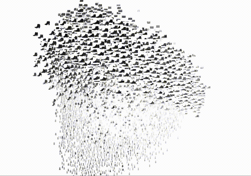 - First, UMAP constructs a high dimensional graph representation of the data using fuzzy simplicial complex: + a representation of a weighted graph, with edge weights representing the likelihood that two points are connected ::: {#fig-simplex} 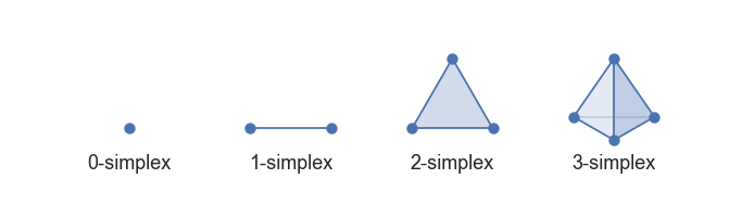 [Low dimensional simplices](https://umap-learn.readthedocs.io/en/latest/how_umap_works.html#id2) ::: - To determine connectedness, UMAP extends a radius outwards from each point, connecting points when those radii overlap. For example, consider a test dataset like this ::: {#fig-sine-wave} 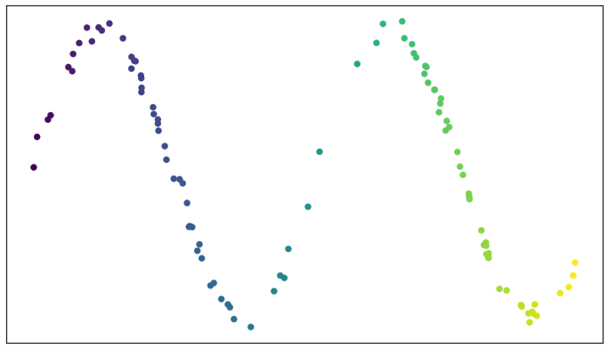 [Test data set of a noisy sine wave](https://umap-learn.readthedocs.io/en/latest/how_umap_works.html#id3) ::: - Then the result is something like this ::: {#fig-open-cover} 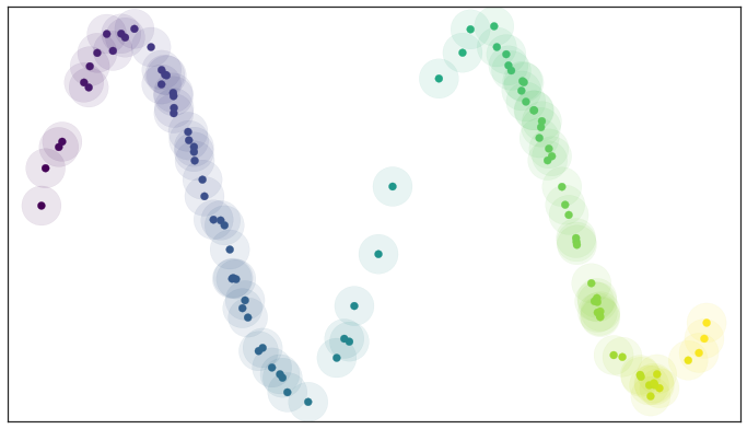 [A basic open cover of the test data](https://umap-learn.readthedocs.io/en/latest/how_umap_works.html#id4) ::: - We can then depict the the simplicial complex of 0-, 1-, and 2-simplices as points, lines, and triangles. ::: {#fig-open-cover} 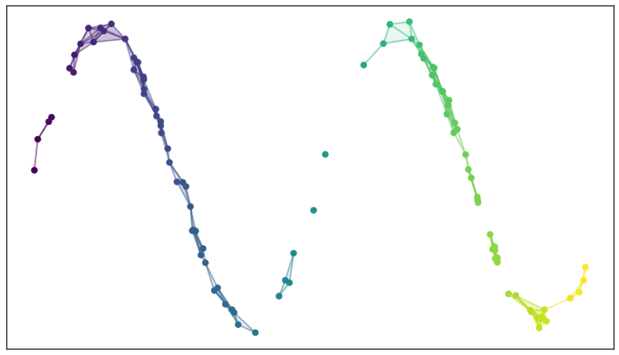 [A simplicial complex built from the test data](https://umap-learn.readthedocs.io/en/latest/how_umap_works.html#id5) ::: - Choosing this radius is critical - too small a choice will lead to small, isolated clusters, while too large a choice will connect everything together. - UMAP overcomes this challenge by choosing a radius locally, based on the distance to each point's nth nearest neighbor, i.e., `n_neighbors`. - UMAP then makes the graph "fuzzy" by decreasing the likelihood of connection as the radius grows. - By stipulating that each point must be connected to at least its closest neighbor, UMAP ensures that local structure is preserved in balance with global structure. - Then, UMAP optimizes a low-dimensional graph to be as structurally similar as possible by controlling the number of edges and their weights. - The second parameter we’ll investigate is `min_dist`, or the minimum distance between points in low-dimensional space. This parameter controls how tightly UMAP clumps points together, with low values leading to more tightly packed embeddings. Larger values of min_dist will make UMAP pack points together more loosely, focusing instead on the preservation of the broad topological structure. #### Try UMAP with different `n_neighbors` and `min_dist` - Let's try:{width=600px height=350px}
- Let $C_1,\ldots,C_K$ denote sets containing the indices of the observations in each cluster. These sets satisfy two properties: 1. $C_1 \cup C_2 \cup \ldots \cup C_K = \{1,\ldots,n\}$. In other words, each observation belongs to at least one of the $K$ clusters. 2. $C_k \cap C_{k'} = \emptyset$ for all $k \ne k'$. In other words, the clusters are non-overlapping: no observation belongs to more than one cluster. For instance, if the $i$th observation is in the $k$th cluster, then $i \in C_k$. - The idea behind $K$-means clustering is that a **good** clustering is one for which the **within-cluster variation** is as small as possible. - The within-cluster variation for cluster $C_k$ is a measure WCV($C_k$) of the amount by which the observations within a cluster differ from each other. - Hence we want to solve the problem $$ \min_{C_1,\ldots,C_K} \left\{ \sum_{i=1}^K \text{WCV}(C_k) \right\}. $$ In words, this formula says that we want to partition the observations into $K$ clusters such that the total within-cluster variation, summed over all $K$ clusters, is as small as possible. - Typically we use Euclidean distance $$ \text{WCV}(C_k) = \frac{1}{|C_k|} \sum_{i, i' \in C_k} \sum_{j=1}^p (x_{ij} - x_{i'j})^2, $$ where $|C_k|$ denotes the number of observations in the $k$th cluster. - Therefore the optimization problem that defines $K$-means clustering is $$ \min_{C_1,\ldots,C_K} \left\{ \sum_{i=1}^K \frac{1}{|C_k|} \sum_{i, i' \in C_k} \sum_{j=1}^p (x_{ij} - x_{i'j})^2 \right\}. $$ - $K$-means clustering algorithm: 1. Randomly assign a number, from 1 to $K$, to each of the observations. These serve as initial cluster assignments for the observations 2. Iterate until the cluster assignments stop changing: 2.a. For each of the $K$ clusters, compute the cluster **centroid**. The $k$th cluster centroid is the vector of the $p$ feature means for the observations in the $k$th cluster. 2.b. Assign each observation to the cluster whose centroid is closest (where **closest** is defined using Euclidean distance). - This algorithm is guaranteed to decrease the value of the objective at each step. Why? Note that $$ \frac{1}{|C_k|} \sum_{i, i' \in C_k} \sum_{j=1}^p (x_{ij} - x_{i'j})^2 = 2 \sum_{i \in C_k} \sum_{j=1}^p (x_{ij} - \bar{x}_{kj})^2, $$ where $\bar{x}_{kj} = \frac{1}{|C_k|} \sum_{i \in C_k} x_{ij}$ is the mean for for feature $j$ in cluster $C_k$. However it is not guaranteed to give the global minimum.{width=600px height=700px}
- Different staring values.{width=600px height=700px}
### Hierarchical clustering - $K$-means clustering requires us to pre-specify the number of clusters $K$. This can be a disadvantage (later we discuss strategies for choosing $K$). - **Hierarchical clustering** is an alternative approach which does not require that we commit to a particular choice of $K$. - We describe **bottom-up** or **agglomerative** clustering. This is the most common type of hierarchical clustering, and refers to the fact that a dendrogram is built starting from the leaves and combining clusters up to the trunk. - Hierarchical clustering algorithm - Start with each point in its own cluster. - Identify the closest two clusters and merge them. - Repeat. - Ends when all points are in a single cluster. - An example. ::: {#figure-bottom-up}{width=500px height=500px}
45 observations generated in 2-dimensional space. In reality there are three distinct classes, shown in separate colors. However, we will treat these class labels as unknown and will seek to cluster the observations in order to discover the classes from the data. ::: ::: {#figure-bottom-up}{width=600px height=450px}
Left: Dendrogram obtained from hierarchically clustering the data from previous slide, with complete linkage and Euclidean distance. Center: The dendrogram from the left-hand panel, cut at a height of 9 (indicated by the dashed line). This cut results in two distinct clusters, shown in different colors. Right: The dendrogram from the left-hand panel, now cut at a height of 5. This cut results in three distinct clusters, shown in different colors. Note that the colors were not used in clustering, but are simply used for display purposes in this figure. ::: - Types of linkage. | _Linkage_ | _Description_ | |-----------|------------------------------------------------------------------------------------------------------------------------------------------------------------------------------------------------------| | Complete | Maximal inter-cluster dissimilarity. Compute all pairwise dissimilarities between the observations in cluster A and the observations in cluster B, and record the **largest** of these dissimilarities. | | Single | Minimal inter-cluster dissimilarity. Compute all pairwise dissimilarities between the observations in cluster A and the observations in cluster B, and record the **smallest** of these dissimilarities. | | Average | Mean inter-cluster dissimilarity. Compute all pairwise dissimilarities between the observations in cluster A and the observations in cluster B, and record the **average** of these dissimilarities. | | Centroid | Dissimilarity between the centroid for cluster A (a mean vector of length $p$) and the centroid for cluster B. Centroid linkage can result in undesirable **inversions**. | - Choice of dissimilarity measure. - So far have used Euclidean distance. - An alternative is **correlation-based distance** which considers two observations to be similar if their features are highly correlated. - Practical issues. - Scaling of the variables matters! - What dissimilarity measure should be used? - What type of linkage should be used? - How many clusters to choose? - Which features should we use to drive the clustering? ## Conclusions - **Unsupervised learning** is important for understanding the variation and grouping structure of a set of unlabeled data, and can be a useful pre-processor for supervised learning. - It is intrinsically more difficult than **supervised learning** because there is no gold standard (like an outcome variable) and no single objective (like test set accuracy). - It is an active field of research, with many recently developed tools such as **self-organizing maps**, **independent components analysis** (ICA) and **spectral clustering**. See ESL Chapter 14.