---
title: Some Applications
subtitle: Biostat 216
author: Dr. Hua Zhou @ UCLA
date: today
format:
  html:
    theme: cosmo
    embed-resources: true
    number-sections: true
    toc: true
    toc-depth: 4
    toc-location: left
    code-fold: false
jupyter:
  jupytext:
    formats: 'ipynb,qmd'
    text_representation:
      extension: .qmd
      format_name: quarto
      format_version: '1.0'
      jupytext_version: 1.15.2
  kernelspec:
    display_name: Julia 1.9.3
    language: julia
    name: julia-1.9
---

```{julia}
using Pkg
Pkg.activate(pwd())
Pkg.instantiate()
Pkg.status()
```

## Matrix completion

Load the 128×128 Lena picture with missing pixels.

```{julia}
using FileIO, Images

lena = load("lena128missing.png")
```

```{julia}
# convert to real matrices
Y = Float64.(lena)
```

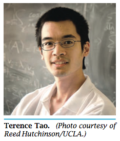
We fill out the missing pixels uisng a **matrix completion** technique developed by Candes and Tao
$$
    \text{minimize } \|\mathbf{X}\|_*
$$
$$
    \text{subject to } x_{ij} = y_{ij} \text{ for all observed entries } (i, j).
$$
Here $\|\mathbf{M}\|_* = \sum_i \sigma_i(\mathbf{M})$ is the nuclear norm. In words we seek the matrix with minimal nuclear norm that agrees with the observed entries. This is a semidefinite programming (SDP) problem readily solved by modern convex optimization software.

We use the convex optimizaion package COSMO.jl to solve for this semi-definite program.

```{julia}
# # Use COSMO solver
using Convex, COSMO
solver = COSMO.Optimizer()


# Linear indices of obs. entries
obsidx = findall(Y[:] .≠ 0.0)
# Create optimization variables
X = Variable(size(Y))
# Set up optmization problem
problem = minimize(nuclearnorm(X))
problem.constraints += X[obsidx] == Y[obsidx]
# Solve the problem by calling solve
@time solve!(problem, solver) # fast
```

```{julia}
colorview(Gray, X.value)
```

## Compressed sensing

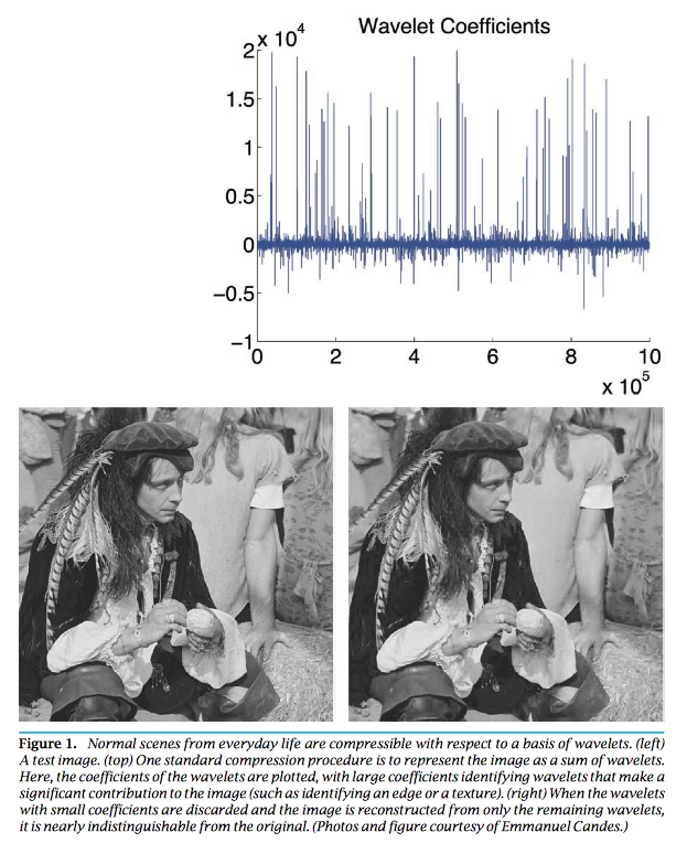
* **Compressed sensing** [Candes and Tao (2006)](https://doi.org/10.1109/TIT.2006.885507) and [Donoho (2006)](https://doi.org/10.1109/TIT.2006.871582) tries to address a fundamental question: how to compress and transmit a complex signal (e.g., musical clips, mega-pixel images), which can be decoded to recover the original signal?

<img src="./david-donoho.jpg" width="100"/>
<img src="./emmanuel-candes.png" width="100"/>
<img src="./terrence-tao.png" width="100"/>

* Suppose a signal $\mathbf{x} \in \mathbb{R}^n$ is sparse with $s$ non-zeros. We under-sample the signal by multiplying a (flat) measurement matrix $\mathbf{y} = \mathbf{A} \mathbf{x}$, where $\mathbf{A} \in \mathbb{R}^{m\times n}$ has iid normal entries. [Candes, Romberg and Tao (2006)](https://doi.org/10.1002/cpa.20124) show that the solution to
$$
\begin{eqnarray*}
	&\text{minimize}& \|\mathbf{x}\|_1 \\
	&\text{subject to}& \mathbf{A} \mathbf{x} = \mathbf{y}
\end{eqnarray*}
$$
exactly recovers the true signal under certain conditions on $\mathbf{A}$ when $n \gg s$ and $m \approx s \ln(n/s)$. Why sparsity is a reasonable assumption? _Virtually all real-world images have low information content_.

<img src="./movie-scene.png" width="400"/>

Generate a sparse signal and sub-sampling:

```{julia}
using CairoMakie, Makie, Random

# random seed
Random.seed!(123)
# Size of signal
n = 1024
# Sparsity (# nonzeros) in the signal
s = 10
# Number of samples (undersample by a factor of 8) 
m = 128

# Generate and display the signal
x0 = zeros(n)
x0[rand(1:n, s)] = randn(s)
# Generate the random sampling matrix
A = randn(m, n) / m
# Subsample by multiplexing
y = A * x0

# plot the true signal
f = Figure()
Makie.Axis(
    f[1, 1], 
    title = "True Signal x0",
    xlabel = "x",
    ylabel = "y"
)
lines!(1:n, x0)
f
```

Solve the linear programming problem.

```{julia}
# Use COSMO solver
solver = COSMO.Optimizer()
# MOI.set(solver, MOI.RawOptimizerAttribute("max_iter"), 5000)

# Set up optimizaiton problem
x = Variable(n)
problem = minimize(norm(x, 1))
problem.constraints += A * x == y

# Solve the problem
@time solve!(problem, solver)
```

```{julia}
# Display the solution
f = Figure()
Makie.Axis(
    f[1, 1], 
    title = "Reconstructed signal overlayed with x0",
    xlabel = "x",
    ylabel = "y"
)
scatter!(1:n, x0, label = "truth")
lines!(1:n, vec(x.value), label = "recovery")
axislegend(position = :lt)
f
```

## Automatic differentiation (Auto-Diff)

Last week we scratched the surface of matrix/vector calculus and chain rules. Recent surge of machine learning sparked rapid advancement of automatic differentiation, which applies chain rule to the computer code to obtain exact gradients (up to machine precision).

### Example: multivariate normal

Define log-likelihood function.

```{julia}
using Distributions, DistributionsAD, LinearAlgebra, PDMats, Random, Zygote

Random.seed!(216)
n, p = 100, 3
Y = randn(p, n) # each column of Y is a sample
```

```{julia}
# log-likelihood evaluator
mnlogl = (θ) -> loglikelihood(MvNormal(θ[:μ], θ[:Ω]), Y)
```

```{julia}
# log-likelihood at (μ = 0, Ω = I)
θ = (μ = zeros(p), Ω = Matrix{Float64}(I(p)))
mnlogl(θ)
```

Calculate gradient by auto-diff.

```{julia}
# gradient of log-likeliohod at (μ = 0, Ω = I)
θ̄ = Zygote.gradient(mnlogl, θ)[1];
```

```{julia}
θ̄[:μ]
```

```{julia}
θ̄[:Ω]
```

Let us check whether auto-diff yields the same answer as our analytical derivations.

```{julia}
# analytical gradient dL/dμ = Ω^{-1} ∑ᵢ (yᵢ - μ)
θ̄[:μ] ≈ θ[:Ω] \ sum(Y .- θ[:μ], dims = 2)
```

```{julia}
# analytical gradient dL/dΩ = -n/2 Ω^{-1} + 1/2 Ω^{-1} ∑ᵢ (yᵢ - μ)(yᵢ - μ)' Ω^{-1}
θ̄[:Ω] ≈ - (n/2) * inv(θ[:Ω]) + 0.5 * inv(θ[:Ω]) * ((Y .- θ[:μ]) * (Y .- θ[:μ])') * inv(θ[:Ω])
```

Surprise! Gradients of the covariance matrix do not match. Close inspection reveals that Julia calculates the gradient with respect to the upper triangular part of the covariance matrix $\text{vech}(\Omega)$

```{julia}
# gradient with respect to vech(Ω)
θ̄[:Ω]
```

```{julia}
# gradient wrt vec(Ω)
- (n/2) * inv(θ[:Ω]) + 0.5 * inv(θ[:Ω]) * ((Y .- θ[:μ]) * (Y .- θ[:μ])') * inv(θ[:Ω])
```

### Example: factor analysis

Now let's try the more complicated factor analysis, where $\boldsymbol{\Omega} = \mathbf{F} \mathbf{F}' + \mathbf{D}$.

```{julia}
# log-likelihood evaluator
falogl = (θ) -> loglikelihood(MvNormal(θ[:F] * θ[:F]' + diagm(θ[:d])), Y)
```

```{julia}
r = 2
# log-likelihood at (F = ones(p, 2), d = ones(p))
θ = (F = ones(p, r), d = ones(p))
falogl(θ)
```

```{julia}
# gradient of log-likeliohod at (F = ones(p, 2), d = ones(p))
θ̄ = Zygote.gradient(falogl, θ)[1];
```

```{julia}
# auto-diff gradient wrt F
θ̄[:F]
```

```{julia}
# analytic gradient wrt F
Ω = θ[:F] * θ[:F]' + diagm(θ[:d])
S = Y * Y' / n
- n * inv(Ω) * θ[:F] + n * inv(Ω) * S * inv(Ω) * θ[:F]
```

```{julia}
# auto-diff gradient wrt d
θ̄[:d]
```

```{julia}
# analytic gradient wrt d
- (n / 2) * diag(inv(Ω) -  inv(Ω) * S * inv(Ω))
```

Hessian (second derivatives) is essentially gradient of gradient. ForwardDiff.jl is better for Hessian calculation.

```{julia}
using ForwardDiff

# HFF = ∂²L/∂F∂F'
ForwardDiff.jacobian(F -> Zygote.gradient(falogl, (F = F, d = ones(p)))[1][:F], θ[:F])
```

```{julia}
# Hdd = ∂²L/∂d∂d'
ForwardDiff.jacobian(d -> Zygote.gradient(falogl, (F = θ[:F], d = d))[1][:d], θ[:d])
```

```{julia}
# Hθθ = ∂²L/∂θ∂θ'

# gradient function with vector input and vector output
falogl_grad = function(θvec)
    θ = (F = reshape(θvec[1:(p * r)], p, r), d = θvec[(p * r + 1):(p * r + p)])
    θ̄ = Zygote.gradient(falogl, θ)[1]
    return [vec(θ̄[:F]); vec(θ̄[:d])]
end

ForwardDiff.jacobian(falogl_grad, [vec(θ[:F]); vec(θ[:d])])
```