---
title: Introduction to Julia
subtitle: Biostat/Biomath M257
author: Dr. Hua Zhou @ UCLA
date: today
format:
html:
theme: cosmo
embed-resources: true
number-sections: true
toc: true
toc-depth: 4
toc-location: left
code-fold: false
jupyter:
jupytext:
formats: 'ipynb,qmd'
text_representation:
extension: .qmd
format_name: quarto
format_version: '1.0'
jupytext_version: 1.14.5
kernelspec:
display_name: Julia 1.8.5
language: julia
name: julia-1.8
---
 System information (for reproducibility)
```{julia}
versioninfo()
```
Load packages:
```{julia}
using Pkg
Pkg.activate(pwd())
Pkg.instantiate()
Pkg.status()
```
```{julia}
using BenchmarkTools, Distributions, RCall
using LinearAlgebra, Profile, SparseArrays
```
## What's Julia?
> Julia is a high-level, high-performance dynamic programming language for technical computing, with syntax that is familiar to users of other technical computing environments
* History:
- Project started in 2009. First public release in 2012
- Creators: Jeff Bezanson, Alan Edelman, Stefan Karpinski, Viral Shah
- First major release v1.0 was released on Aug 8, 2018
- Current stable release v1.8.5 (as of Apr 6, 2023)
* Aim to solve the notorious **two language problem**: Prototype code goes into high-level languages like R/Python, production code goes into low-level language like C/C++.
Julia aims to:
> Walks like Python. Runs like C.
System information (for reproducibility)
```{julia}
versioninfo()
```
Load packages:
```{julia}
using Pkg
Pkg.activate(pwd())
Pkg.instantiate()
Pkg.status()
```
```{julia}
using BenchmarkTools, Distributions, RCall
using LinearAlgebra, Profile, SparseArrays
```
## What's Julia?
> Julia is a high-level, high-performance dynamic programming language for technical computing, with syntax that is familiar to users of other technical computing environments
* History:
- Project started in 2009. First public release in 2012
- Creators: Jeff Bezanson, Alan Edelman, Stefan Karpinski, Viral Shah
- First major release v1.0 was released on Aug 8, 2018
- Current stable release v1.8.5 (as of Apr 6, 2023)
* Aim to solve the notorious **two language problem**: Prototype code goes into high-level languages like R/Python, production code goes into low-level language like C/C++.
Julia aims to:
> Walks like Python. Runs like C.
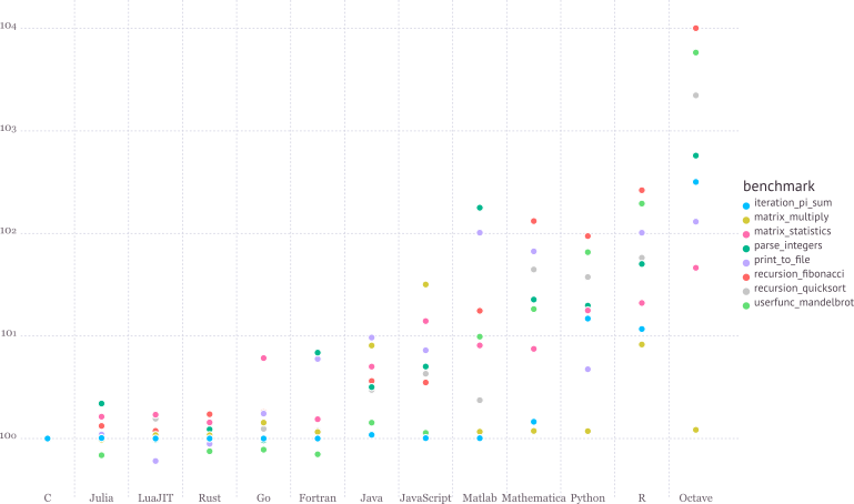 See for the details of benchmark.
* Write high-level, abstract code that closely resembles mathematical formulas
- yet produces fast, low-level machine code that has traditionally only been generated by static languages.
* Julia is more than just "Fast R" or "Fast Matlab"
- Performance comes from features that work well together.
- You can't just take the magic dust that makes Julia fast and sprinkle it on [language of choice]
## Learning resources
1. The (free) online course [Introduction to Julia](https://juliaacademy.com/p/intro-to-julia), by Jane Herriman.
2. Cheat sheet: [The Fast Track to Julia](https://juliadocs.github.io/Julia-Cheat-Sheet/).
3. Browse the Julia [documentation](https://docs.julialang.org/en).
bm
4. For Matlab users, read [Noteworthy Differences From Matlab](https://docs.julialang.org/en/v1/manual/noteworthy-differences/#Noteworthy-differences-from-MATLAB-1).
For R users, read [Noteworthy Differences From R](https://docs.julialang.org/en/v1/manual/noteworthy-differences/#Noteworthy-differences-from-R-1).
For Python users, read [Noteworthy Differences From Python](https://docs.julialang.org/en/v1/manual/noteworthy-differences/?highlight=matlab#Noteworthy-differences-from-Python-1).
5. The [Learning page](http://julialang.org/learning/) on Julia's website has pointers to many other learning resources.
## Julia REPL (Read-Evaluation-Print-Loop)
The `Julia` REPL, or `Julia` shell, has at least five modes.
1. **Default mode** is the Julian prompt `julia>`. Type backspace in other modes to enter default mode.
2. **Help mode** `help?>`. Type `?` to enter help mode. `?search_term` does a fuzzy search for `search_term`.
3. **Shell mode** `shell>`. Type `;` to enter shell mode.
4. **Package mode** `(@v1.8) pkg>`. Type `]` to enter package mode for managing Julia packages (install, uninstall, update, ...).
5. **Search mode** `(reverse-i-search)`. Press `ctrl+R` to enter search model.
6. With `RCall.jl` package installed, we can enter the **R mode** by typing `$` (shift+4) at Julia REPL.
Some survival commands in Julia REPL:
1. `exit()` or `Ctrl+D`: exit Julia.
2. `Ctrl+C`: interrupt execution.
3. `Ctrl+L`: clear screen.
0. Append `;` (semi-colon) to suppress displaying output from a command. Same as Matlab.
0. `include("filename.jl")` to source a Julia code file.
## Seek help
* Online help from REPL: `?function_name`.
* Google.
* Julia documentation: .
* Look up source code: `@edit sin(π)`.
* Discourse: .
* Friends.
## Which IDE?
* Julia homepage lists many choices: Juno, VS Code, Vim, ...
* Unfortunately at the moment there are no mature RStudio- or Matlab-like IDE for Julia yet.
* For dynamic document, e.g., homework, I recommend [Jupyter Notebook](https://jupyter.org/install.html) or [JupyterLab](http://jupyterlab.readthedocs.io/en/stable/).
* For extensive Julia coding, myself has been happily using the editor [VS Code](https://code.visualstudio.com) with extensions `Julia` and `VS Code Jupyter Notebook Previewer` installed.
## Julia package system
* Each Julia package is a Git repository. Each Julia package name ends with `.jl`. E.g., `Distributions.jl` package lives at .
Google search with `PackageName.jl` usually leads to the package on github.com.
* The package ecosystem is rapidly maturing; a complete list of **registered** packages (which are required to have a certain level of testing and documentation) is at [http://pkg.julialang.org/](http://pkg.julialang.org/).
* For example, the package called `Distributions.jl` is added with
```julia
# in Pkg mode
(@v1.8) pkg> add Distributions
```
and "removed" (although not completely deleted) with
```julia
# in Pkg mode
(@v1.8) pkg> rm Distributions
```
* The package manager provides a dependency solver that determines which packages are actually required to be installed.
* **Non-registered** packages are added by cloning the relevant Git repository. E.g.,
```julia
# in Pkg mode
(@v1.8) pkg> add https://github.com/OpenMendel/SnpArrays.jl
```
* A package needs only be added once, at which point it is downloaded into your local `.julia/packages` directory in your home directory.
```{julia}
readdir(Sys.islinux() ? ENV["JULIA_PATH"] * "/pkg/packages" : ENV["HOME"] * "/.julia/packages")
```
* Directory of a specific package can be queried by `pathof()`:
```{julia}
pathof(Distributions)
```
* If you start having problems with packages that seem to be unsolvable, you may try just deleting your .julia directory and reinstalling all your packages.
* Periodically, one should run `update` in Pkg mode, which checks for, downloads and installs updated versions of all the packages you currently have installed.
* `status` lists the status of all installed packages.
* Using functions in package.
```julia
using Distributions
```
This pulls all of the *exported* functions in the module into your local namespace, as you can check using the `whos()` command. An alternative is
```julia
import Distributions
```
Now, the functions from the Distributions package are available only using
```julia
Distributions.
```
All functions, not only exported functions, are always available like this.
## Calling R from Julia
* The [`RCall.jl`](https://github.com/JuliaInterop/RCall.jl) package allows us to embed R code inside of Julia.
* There are also `PyCall.jl`, `MATLAB.jl`, `JavaCall.jl`, `CxxWrap.jl` packages for interfacing with other languages.
```{julia}
# x is in Julia workspace
x = randn(1000)
# $ is the interpolation operator
R"""
hist($x, main = "I'm plotting a Julia vector")
""";
```
```{julia}
R"""
library(ggplot2)
qplot($x)
"""
```
```{julia}
x = R"""
rnorm(10)
"""
```
```{julia}
# collect R variable into Julia workspace
y = collect(x)
```
* Access Julia variables in R REPL mode:
```julia
julia> x = rand(5) # Julia variable
R> y <- $x
```
* Pass Julia expression in R REPL mode:
```julia
R> y <- $(rand(5))
```
* Put Julia variable into R environment:
```julia
julia> @rput x
R> x
```
* Get R variable into Julia environment:
```julia
R> r <- 2
Julia> @rget r
```
* If you want to call Julia within R, check out the [`JuliaCall`](https://non-contradiction.github.io/JuliaCall//index.html) package.
## Some basic Julia code
```{julia}
# an integer, same as int in R
y = 1
```
```{julia}
# query type of a Julia object
typeof(y)
```
```{julia}
# a Float64 number, same as double in R
y = 1.0
```
```{julia}
typeof(y)
```
```{julia}
# Greek letters: `\pi`
π
```
```{julia}
typeof(π)
```
```{julia}
# Greek letters: `\theta`
θ = y + π
```
```{julia}
# emoji! `\:kissing_cat:`
😽 = 5.0
😽 + 1
```
```{julia}
# `\alpha\hat`
α̂ = π
```
For a list of unicode symbols that can be tab-completed, see . Or in the help mode, type `?` followed by the unicode symbol you want to input.
```{julia}
# vector of Float64 0s
x = zeros(5)
```
```{julia}
# vector Int64 0s
x = zeros(Int, 5)
```
```{julia}
# matrix of Float64 0s
x = zeros(5, 3)
```
```{julia}
# matrix of Float64 1s
x = ones(5, 3)
```
```{julia}
# define array without initialization
x = Matrix{Float64}(undef, 5, 3)
```
```{julia}
# fill a matrix by 0s
fill!(x, 0)
```
```{julia}
# initialize an array to be constant 2.5
fill(2.5, (5, 3))
```
```{julia}
# rational number
a = 3//5
```
```{julia}
typeof(a)
```
```{julia}
b = 3//7
```
```{julia}
a + b
```
```{julia}
# uniform [0, 1) random numbers
x = rand(5, 3)
```
```{julia}
# uniform random numbers (in single precision)
x = rand(Float16, 5, 3)
```
```{julia}
# random numbers from {1,...,5}
x = rand(1:5, 5, 3)
```
```{julia}
# standard normal random numbers
x = randn(5, 3)
```
```{julia}
# range
1:10
```
```{julia}
typeof(1:10)
```
```{julia}
1:2:10
```
```{julia}
typeof(1:2:10)
```
```{julia}
# integers 1-10
x = collect(1:10)
```
```{julia}
# or equivalently
[1:10...]
```
```{julia}
# Float64 numbers 1-10
x = collect(1.0:10)
```
```{julia}
# convert to a specific type
convert(Vector{Float64}, 1:10)
```
## Matrices and vectors
### Dimensions
```{julia}
x = randn(5, 3)
```
```{julia}
size(x)
```
```{julia}
size(x, 1) # nrow() in R
```
```{julia}
size(x, 2) # ncol() in R
```
```{julia}
# total number of elements
length(x)
```
### Indexing
```{julia}
# 5 × 5 matrix of random Normal(0, 1)
x = randn(5, 5)
```
```{julia}
# first column
x[:, 1]
```
```{julia}
# first row
x[1, :]
```
```{julia}
# sub-array
x[1:2, 2:3]
```
```{julia}
# getting a subset of a matrix creates a copy, but you can also create "views"
z = view(x, 1:2, 2:3)
```
```{julia}
# same as
@views z = x[1:2, 2:3]
```
```{julia}
# change in z (view) changes x as well
z[2, 2] = 0.0
x
```
```{julia}
# y points to same data as x
y = x
```
```{julia}
# x and y point to same data
pointer(x), pointer(y)
```
```{julia}
# changing y also changes x
y[:, 1] .= 0
x
```
```{julia}
# create a new copy of data
z = copy(x)
```
```{julia}
pointer(x), pointer(z)
```
### Concatenate matrices
```{julia}
# 3-by-1 vector
[1, 2, 3]
```
```{julia}
# 1-by-3 array
[1 2 3]
```
```{julia}
# multiple assignment by tuple
x, y, z = randn(5, 3), randn(5, 2), randn(3, 5)
```
```{julia}
[x y] # 5-by-5 matrix
```
```{julia}
[x y; z] # 8-by-5 matrix
```
### Dot operation (broadcasting)
Dot operation in Julia is elementwise operation, similar to Matlab.
```{julia}
x = randn(5, 3)
```
```{julia}
y = ones(5, 3)
```
```{julia}
x .* y # same x * y in R
```
```{julia}
x .^ (-2)
```
```{julia}
sin.(x)
```
### Basic linear algebra
```{julia}
x = randn(5)
```
```{julia}
# vector L2 norm
norm(x)
```
```{julia}
# same as
sqrt(sum(abs2, x))
```
```{julia}
y = randn(5) # another vector
# dot product
dot(x, y) # x' * y
```
```{julia}
# same as
x'y
```
```{julia}
x, y = randn(5, 3), randn(3, 2)
# matrix multiplication, same as %*% in R
x * y
```
```{julia}
x = randn(3, 3)
```
```{julia}
# conjugate transpose
x'
```
```{julia}
b = rand(3)
x'b # same as x' * b
```
```{julia}
# trace
tr(x)
```
```{julia}
det(x)
```
```{julia}
rank(x)
```
### Sparse matrices
```{julia}
# 10-by-10 sparse matrix with sparsity 0.1
X = sprandn(10, 10, .1)
```
```{julia}
# dump() in Julia is like str() in R
dump(X)
```
```{julia}
# convert to dense matrix; be cautious when dealing with big data
Xfull = convert(Matrix{Float64}, X)
```
```{julia}
# convert a dense matrix to sparse matrix
sparse(Xfull)
```
```{julia}
# syntax for sparse linear algebra is same as dense linear algebra
β = ones(10)
X * β
```
```{julia}
# many functions apply to sparse matrices as well
sum(X)
```
## Control flow and loops
* if-elseif-else-end
```julia
if condition1
# do something
elseif condition2
# do something
else
# do something
end
```
* `for` loop
```julia
for i in 1:10
println(i)
end
```
* Nested `for` loop:
```julia
for i in 1:10
for j in 1:5
println(i * j)
end
end
```
Same as
```julia
for i in 1:10, j in 1:5
println(i * j)
end
```
* Exit loop:
```julia
for i in 1:10
# do something
if condition1
break # skip remaining loop
end
end
```
* Exit iteration:
```julia
for i in 1:10
# do something
if condition1
continue # skip to next iteration
end
# do something
end
```
## Functions
* In Julia, all arguments to functions are **passed by reference**, in contrast to R and Matlab.
* Function names ending with `!` indicates that function mutates at least one argument, typically the first.
```julia
sort!(x) # vs sort(x)
```
* Function definition
```julia
function func(req1, req2; key1=dflt1, key2=dflt2)
# do stuff
return out1, out2, out3
end
```
**Required arguments** are separated with a comma and use the positional notation.
**Optional arguments** need a default value in the signature.
**Semicolon** is not required in function call.
**return** statement is optional.
Multiple outputs can be returned as a **tuple**, e.g., `return out1, out2, out3`.
* Anonymous functions, e.g., `x -> x^2`, is commonly used in collection function or list comprehensions.
```julia
map(x -> x^2, y) # square each element in x
```
* Functions can be nested:
```julia
function outerfunction()
# do some outer stuff
function innerfunction()
# do inner stuff
# can access prior outer definitions
end
# do more outer stuff
end
```
* Functions can be vectorized using the Dot syntax:
```{julia}
# defined for scalar
function myfunc(x)
return sin(x^2)
end
x = randn(5, 3)
myfunc.(x)
```
* **Collection function** (think this as the series of `apply` functions in R).
Apply a function to each element of a collection:
```julia
map(f, coll) # or
map(coll) do elem
# do stuff with elem
# must contain return
end
```
```{julia}
map(x -> sin(x^2), x)
```
```{julia}
map(x) do elem
elem = elem^2
return sin(elem)
end
```
```{julia}
# Mapreduce
mapreduce(x -> sin(x^2), +, x)
```
```{julia}
# same as
sum(x -> sin(x^2), x)
```
* List **comprehension**
```{julia}
[sin(2i + j) for i in 1:5, j in 1:3] # similar to Python
```
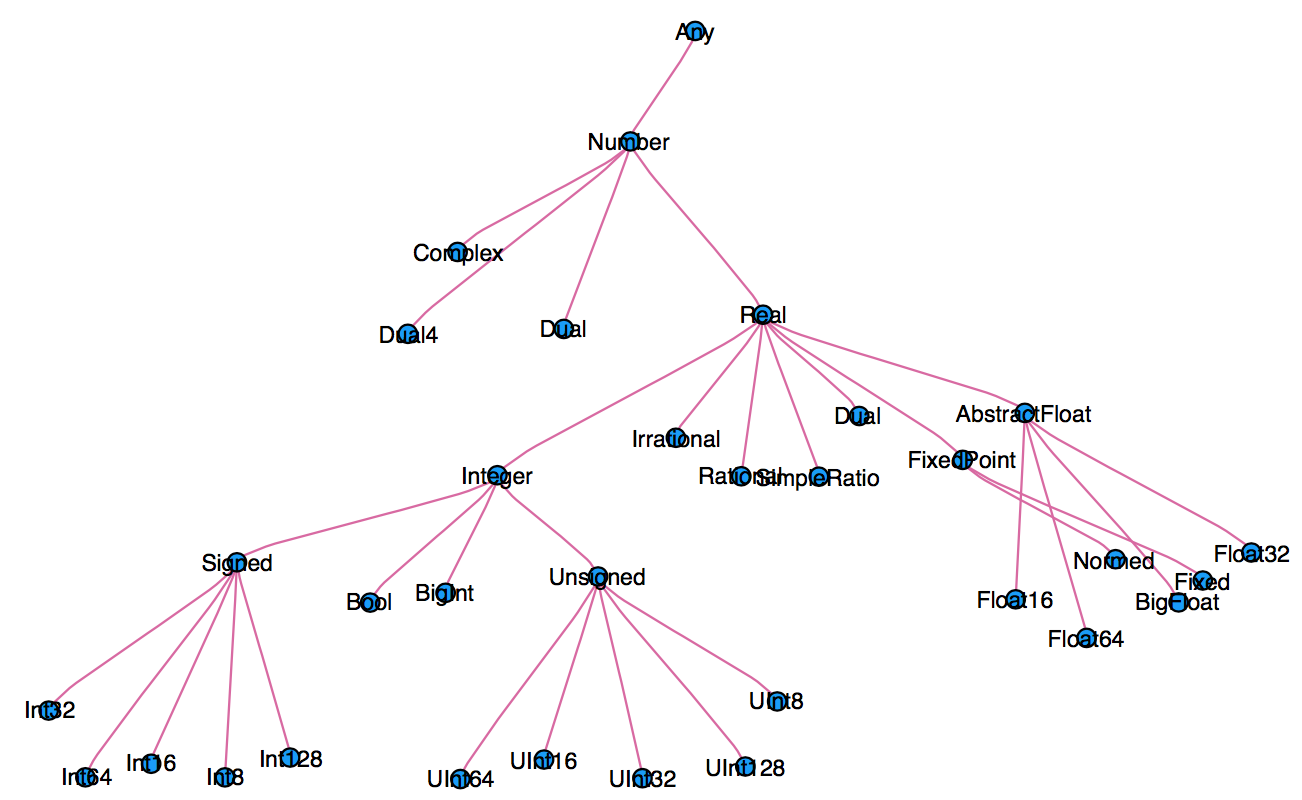
## Type system
* Every variable in Julia has a type.
* When thinking about types, think about sets.
* Everything is a subtype of the abstract type `Any`.
* An abstract type defines a set of types
- Consider types in Julia that are a `Number`:
See for the details of benchmark.
* Write high-level, abstract code that closely resembles mathematical formulas
- yet produces fast, low-level machine code that has traditionally only been generated by static languages.
* Julia is more than just "Fast R" or "Fast Matlab"
- Performance comes from features that work well together.
- You can't just take the magic dust that makes Julia fast and sprinkle it on [language of choice]
## Learning resources
1. The (free) online course [Introduction to Julia](https://juliaacademy.com/p/intro-to-julia), by Jane Herriman.
2. Cheat sheet: [The Fast Track to Julia](https://juliadocs.github.io/Julia-Cheat-Sheet/).
3. Browse the Julia [documentation](https://docs.julialang.org/en).
bm
4. For Matlab users, read [Noteworthy Differences From Matlab](https://docs.julialang.org/en/v1/manual/noteworthy-differences/#Noteworthy-differences-from-MATLAB-1).
For R users, read [Noteworthy Differences From R](https://docs.julialang.org/en/v1/manual/noteworthy-differences/#Noteworthy-differences-from-R-1).
For Python users, read [Noteworthy Differences From Python](https://docs.julialang.org/en/v1/manual/noteworthy-differences/?highlight=matlab#Noteworthy-differences-from-Python-1).
5. The [Learning page](http://julialang.org/learning/) on Julia's website has pointers to many other learning resources.
## Julia REPL (Read-Evaluation-Print-Loop)
The `Julia` REPL, or `Julia` shell, has at least five modes.
1. **Default mode** is the Julian prompt `julia>`. Type backspace in other modes to enter default mode.
2. **Help mode** `help?>`. Type `?` to enter help mode. `?search_term` does a fuzzy search for `search_term`.
3. **Shell mode** `shell>`. Type `;` to enter shell mode.
4. **Package mode** `(@v1.8) pkg>`. Type `]` to enter package mode for managing Julia packages (install, uninstall, update, ...).
5. **Search mode** `(reverse-i-search)`. Press `ctrl+R` to enter search model.
6. With `RCall.jl` package installed, we can enter the **R mode** by typing `$` (shift+4) at Julia REPL.
Some survival commands in Julia REPL:
1. `exit()` or `Ctrl+D`: exit Julia.
2. `Ctrl+C`: interrupt execution.
3. `Ctrl+L`: clear screen.
0. Append `;` (semi-colon) to suppress displaying output from a command. Same as Matlab.
0. `include("filename.jl")` to source a Julia code file.
## Seek help
* Online help from REPL: `?function_name`.
* Google.
* Julia documentation: .
* Look up source code: `@edit sin(π)`.
* Discourse: .
* Friends.
## Which IDE?
* Julia homepage lists many choices: Juno, VS Code, Vim, ...
* Unfortunately at the moment there are no mature RStudio- or Matlab-like IDE for Julia yet.
* For dynamic document, e.g., homework, I recommend [Jupyter Notebook](https://jupyter.org/install.html) or [JupyterLab](http://jupyterlab.readthedocs.io/en/stable/).
* For extensive Julia coding, myself has been happily using the editor [VS Code](https://code.visualstudio.com) with extensions `Julia` and `VS Code Jupyter Notebook Previewer` installed.
## Julia package system
* Each Julia package is a Git repository. Each Julia package name ends with `.jl`. E.g., `Distributions.jl` package lives at .
Google search with `PackageName.jl` usually leads to the package on github.com.
* The package ecosystem is rapidly maturing; a complete list of **registered** packages (which are required to have a certain level of testing and documentation) is at [http://pkg.julialang.org/](http://pkg.julialang.org/).
* For example, the package called `Distributions.jl` is added with
```julia
# in Pkg mode
(@v1.8) pkg> add Distributions
```
and "removed" (although not completely deleted) with
```julia
# in Pkg mode
(@v1.8) pkg> rm Distributions
```
* The package manager provides a dependency solver that determines which packages are actually required to be installed.
* **Non-registered** packages are added by cloning the relevant Git repository. E.g.,
```julia
# in Pkg mode
(@v1.8) pkg> add https://github.com/OpenMendel/SnpArrays.jl
```
* A package needs only be added once, at which point it is downloaded into your local `.julia/packages` directory in your home directory.
```{julia}
readdir(Sys.islinux() ? ENV["JULIA_PATH"] * "/pkg/packages" : ENV["HOME"] * "/.julia/packages")
```
* Directory of a specific package can be queried by `pathof()`:
```{julia}
pathof(Distributions)
```
* If you start having problems with packages that seem to be unsolvable, you may try just deleting your .julia directory and reinstalling all your packages.
* Periodically, one should run `update` in Pkg mode, which checks for, downloads and installs updated versions of all the packages you currently have installed.
* `status` lists the status of all installed packages.
* Using functions in package.
```julia
using Distributions
```
This pulls all of the *exported* functions in the module into your local namespace, as you can check using the `whos()` command. An alternative is
```julia
import Distributions
```
Now, the functions from the Distributions package are available only using
```julia
Distributions.
```
All functions, not only exported functions, are always available like this.
## Calling R from Julia
* The [`RCall.jl`](https://github.com/JuliaInterop/RCall.jl) package allows us to embed R code inside of Julia.
* There are also `PyCall.jl`, `MATLAB.jl`, `JavaCall.jl`, `CxxWrap.jl` packages for interfacing with other languages.
```{julia}
# x is in Julia workspace
x = randn(1000)
# $ is the interpolation operator
R"""
hist($x, main = "I'm plotting a Julia vector")
""";
```
```{julia}
R"""
library(ggplot2)
qplot($x)
"""
```
```{julia}
x = R"""
rnorm(10)
"""
```
```{julia}
# collect R variable into Julia workspace
y = collect(x)
```
* Access Julia variables in R REPL mode:
```julia
julia> x = rand(5) # Julia variable
R> y <- $x
```
* Pass Julia expression in R REPL mode:
```julia
R> y <- $(rand(5))
```
* Put Julia variable into R environment:
```julia
julia> @rput x
R> x
```
* Get R variable into Julia environment:
```julia
R> r <- 2
Julia> @rget r
```
* If you want to call Julia within R, check out the [`JuliaCall`](https://non-contradiction.github.io/JuliaCall//index.html) package.
## Some basic Julia code
```{julia}
# an integer, same as int in R
y = 1
```
```{julia}
# query type of a Julia object
typeof(y)
```
```{julia}
# a Float64 number, same as double in R
y = 1.0
```
```{julia}
typeof(y)
```
```{julia}
# Greek letters: `\pi`
π
```
```{julia}
typeof(π)
```
```{julia}
# Greek letters: `\theta`
θ = y + π
```
```{julia}
# emoji! `\:kissing_cat:`
😽 = 5.0
😽 + 1
```
```{julia}
# `\alpha\hat`
α̂ = π
```
For a list of unicode symbols that can be tab-completed, see . Or in the help mode, type `?` followed by the unicode symbol you want to input.
```{julia}
# vector of Float64 0s
x = zeros(5)
```
```{julia}
# vector Int64 0s
x = zeros(Int, 5)
```
```{julia}
# matrix of Float64 0s
x = zeros(5, 3)
```
```{julia}
# matrix of Float64 1s
x = ones(5, 3)
```
```{julia}
# define array without initialization
x = Matrix{Float64}(undef, 5, 3)
```
```{julia}
# fill a matrix by 0s
fill!(x, 0)
```
```{julia}
# initialize an array to be constant 2.5
fill(2.5, (5, 3))
```
```{julia}
# rational number
a = 3//5
```
```{julia}
typeof(a)
```
```{julia}
b = 3//7
```
```{julia}
a + b
```
```{julia}
# uniform [0, 1) random numbers
x = rand(5, 3)
```
```{julia}
# uniform random numbers (in single precision)
x = rand(Float16, 5, 3)
```
```{julia}
# random numbers from {1,...,5}
x = rand(1:5, 5, 3)
```
```{julia}
# standard normal random numbers
x = randn(5, 3)
```
```{julia}
# range
1:10
```
```{julia}
typeof(1:10)
```
```{julia}
1:2:10
```
```{julia}
typeof(1:2:10)
```
```{julia}
# integers 1-10
x = collect(1:10)
```
```{julia}
# or equivalently
[1:10...]
```
```{julia}
# Float64 numbers 1-10
x = collect(1.0:10)
```
```{julia}
# convert to a specific type
convert(Vector{Float64}, 1:10)
```
## Matrices and vectors
### Dimensions
```{julia}
x = randn(5, 3)
```
```{julia}
size(x)
```
```{julia}
size(x, 1) # nrow() in R
```
```{julia}
size(x, 2) # ncol() in R
```
```{julia}
# total number of elements
length(x)
```
### Indexing
```{julia}
# 5 × 5 matrix of random Normal(0, 1)
x = randn(5, 5)
```
```{julia}
# first column
x[:, 1]
```
```{julia}
# first row
x[1, :]
```
```{julia}
# sub-array
x[1:2, 2:3]
```
```{julia}
# getting a subset of a matrix creates a copy, but you can also create "views"
z = view(x, 1:2, 2:3)
```
```{julia}
# same as
@views z = x[1:2, 2:3]
```
```{julia}
# change in z (view) changes x as well
z[2, 2] = 0.0
x
```
```{julia}
# y points to same data as x
y = x
```
```{julia}
# x and y point to same data
pointer(x), pointer(y)
```
```{julia}
# changing y also changes x
y[:, 1] .= 0
x
```
```{julia}
# create a new copy of data
z = copy(x)
```
```{julia}
pointer(x), pointer(z)
```
### Concatenate matrices
```{julia}
# 3-by-1 vector
[1, 2, 3]
```
```{julia}
# 1-by-3 array
[1 2 3]
```
```{julia}
# multiple assignment by tuple
x, y, z = randn(5, 3), randn(5, 2), randn(3, 5)
```
```{julia}
[x y] # 5-by-5 matrix
```
```{julia}
[x y; z] # 8-by-5 matrix
```
### Dot operation (broadcasting)
Dot operation in Julia is elementwise operation, similar to Matlab.
```{julia}
x = randn(5, 3)
```
```{julia}
y = ones(5, 3)
```
```{julia}
x .* y # same x * y in R
```
```{julia}
x .^ (-2)
```
```{julia}
sin.(x)
```
### Basic linear algebra
```{julia}
x = randn(5)
```
```{julia}
# vector L2 norm
norm(x)
```
```{julia}
# same as
sqrt(sum(abs2, x))
```
```{julia}
y = randn(5) # another vector
# dot product
dot(x, y) # x' * y
```
```{julia}
# same as
x'y
```
```{julia}
x, y = randn(5, 3), randn(3, 2)
# matrix multiplication, same as %*% in R
x * y
```
```{julia}
x = randn(3, 3)
```
```{julia}
# conjugate transpose
x'
```
```{julia}
b = rand(3)
x'b # same as x' * b
```
```{julia}
# trace
tr(x)
```
```{julia}
det(x)
```
```{julia}
rank(x)
```
### Sparse matrices
```{julia}
# 10-by-10 sparse matrix with sparsity 0.1
X = sprandn(10, 10, .1)
```
```{julia}
# dump() in Julia is like str() in R
dump(X)
```
```{julia}
# convert to dense matrix; be cautious when dealing with big data
Xfull = convert(Matrix{Float64}, X)
```
```{julia}
# convert a dense matrix to sparse matrix
sparse(Xfull)
```
```{julia}
# syntax for sparse linear algebra is same as dense linear algebra
β = ones(10)
X * β
```
```{julia}
# many functions apply to sparse matrices as well
sum(X)
```
## Control flow and loops
* if-elseif-else-end
```julia
if condition1
# do something
elseif condition2
# do something
else
# do something
end
```
* `for` loop
```julia
for i in 1:10
println(i)
end
```
* Nested `for` loop:
```julia
for i in 1:10
for j in 1:5
println(i * j)
end
end
```
Same as
```julia
for i in 1:10, j in 1:5
println(i * j)
end
```
* Exit loop:
```julia
for i in 1:10
# do something
if condition1
break # skip remaining loop
end
end
```
* Exit iteration:
```julia
for i in 1:10
# do something
if condition1
continue # skip to next iteration
end
# do something
end
```
## Functions
* In Julia, all arguments to functions are **passed by reference**, in contrast to R and Matlab.
* Function names ending with `!` indicates that function mutates at least one argument, typically the first.
```julia
sort!(x) # vs sort(x)
```
* Function definition
```julia
function func(req1, req2; key1=dflt1, key2=dflt2)
# do stuff
return out1, out2, out3
end
```
**Required arguments** are separated with a comma and use the positional notation.
**Optional arguments** need a default value in the signature.
**Semicolon** is not required in function call.
**return** statement is optional.
Multiple outputs can be returned as a **tuple**, e.g., `return out1, out2, out3`.
* Anonymous functions, e.g., `x -> x^2`, is commonly used in collection function or list comprehensions.
```julia
map(x -> x^2, y) # square each element in x
```
* Functions can be nested:
```julia
function outerfunction()
# do some outer stuff
function innerfunction()
# do inner stuff
# can access prior outer definitions
end
# do more outer stuff
end
```
* Functions can be vectorized using the Dot syntax:
```{julia}
# defined for scalar
function myfunc(x)
return sin(x^2)
end
x = randn(5, 3)
myfunc.(x)
```
* **Collection function** (think this as the series of `apply` functions in R).
Apply a function to each element of a collection:
```julia
map(f, coll) # or
map(coll) do elem
# do stuff with elem
# must contain return
end
```
```{julia}
map(x -> sin(x^2), x)
```
```{julia}
map(x) do elem
elem = elem^2
return sin(elem)
end
```
```{julia}
# Mapreduce
mapreduce(x -> sin(x^2), +, x)
```
```{julia}
# same as
sum(x -> sin(x^2), x)
```
* List **comprehension**
```{julia}
[sin(2i + j) for i in 1:5, j in 1:3] # similar to Python
```
## Type system
* Every variable in Julia has a type.
* When thinking about types, think about sets.
* Everything is a subtype of the abstract type `Any`.
* An abstract type defines a set of types
- Consider types in Julia that are a `Number`:
 * We can explore type hierarchy with `typeof()`, `supertype()`, and `subtypes()`.
```{julia}
# 1.0: double precision, 1: 64-bit integer
typeof(1.0), typeof(1)
```
```{julia}
supertype(Float64)
```
```{julia}
subtypes(AbstractFloat)
```
```{julia}
# Is Float64 a subtype of AbstractFloat?
Float64 <: AbstractFloat
```
```{julia}
# On 64bit machine, Int == Int64
Int == Int64
```
```{julia}
# convert to Float64
convert(Float64, 1)
```
```{julia}
# same as casting
Float64(1)
```
```{julia}
# Float32 vector
x = randn(Float32, 5)
```
```{julia}
# convert to Float64
convert(Vector{Float64}, x)
```
```{julia}
# same as broadcasting (dot operatation)
Float64.(x)
```
```{julia}
# convert Float64 to Int64
convert(Int, 1.0)
```
```{julia}
convert(Int, 1.5) # should use round(1.5)
```
```{julia}
round(Int, 1.5)
```
## Multiple dispatch
* Multiple dispatch lies in the core of Julia design. It allows built-in and user-defined functions to be overloaded for different combinations of argument types.
* Let's consider a simple "doubling" function:
```{julia}
g(x) = x + x
```
```{julia}
g(1.5)
```
This definition is too broad, since some things, e.g., strings, can't be added
```{julia}
g("hello world")
```
* This definition is correct but too restrictive, since any `Number` can be added.
```{julia}
g(x::Float64) = x + x
```
* This definition will automatically work on the entire type tree above!
```{julia}
g(x::Number) = x + x
```
This is a lot nicer than
```julia
function g(x)
if isa(x, Number)
return x + x
else
throw(ArgumentError("x should be a number"))
end
end
```
* `methods(func)` function display all methods defined for `func`.
```{julia}
methods(g)
```
* When calling a function with multiple definitions, Julia will search from the narrowest signature to the broadest signature.
* `@which func(x)` marco tells which method is being used for argument signature `x`.
```{julia}
# an Int64 input
@which g(1)
```
```{julia}
# a Vector{Float64} input
@which g(randn(5))
```
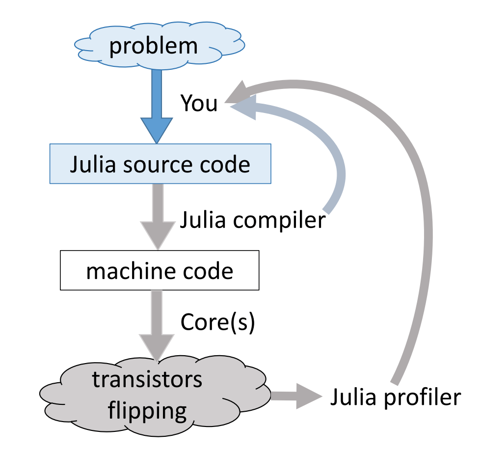
## Just-in-time compilation (JIT)
Following figures are taken from Arch D. Robinson's slides [Introduction to Writing High Performance Julia](https://www.youtube.com/watch?v=szE4txAD8mk).
|
* We can explore type hierarchy with `typeof()`, `supertype()`, and `subtypes()`.
```{julia}
# 1.0: double precision, 1: 64-bit integer
typeof(1.0), typeof(1)
```
```{julia}
supertype(Float64)
```
```{julia}
subtypes(AbstractFloat)
```
```{julia}
# Is Float64 a subtype of AbstractFloat?
Float64 <: AbstractFloat
```
```{julia}
# On 64bit machine, Int == Int64
Int == Int64
```
```{julia}
# convert to Float64
convert(Float64, 1)
```
```{julia}
# same as casting
Float64(1)
```
```{julia}
# Float32 vector
x = randn(Float32, 5)
```
```{julia}
# convert to Float64
convert(Vector{Float64}, x)
```
```{julia}
# same as broadcasting (dot operatation)
Float64.(x)
```
```{julia}
# convert Float64 to Int64
convert(Int, 1.0)
```
```{julia}
convert(Int, 1.5) # should use round(1.5)
```
```{julia}
round(Int, 1.5)
```
## Multiple dispatch
* Multiple dispatch lies in the core of Julia design. It allows built-in and user-defined functions to be overloaded for different combinations of argument types.
* Let's consider a simple "doubling" function:
```{julia}
g(x) = x + x
```
```{julia}
g(1.5)
```
This definition is too broad, since some things, e.g., strings, can't be added
```{julia}
g("hello world")
```
* This definition is correct but too restrictive, since any `Number` can be added.
```{julia}
g(x::Float64) = x + x
```
* This definition will automatically work on the entire type tree above!
```{julia}
g(x::Number) = x + x
```
This is a lot nicer than
```julia
function g(x)
if isa(x, Number)
return x + x
else
throw(ArgumentError("x should be a number"))
end
end
```
* `methods(func)` function display all methods defined for `func`.
```{julia}
methods(g)
```
* When calling a function with multiple definitions, Julia will search from the narrowest signature to the broadest signature.
* `@which func(x)` marco tells which method is being used for argument signature `x`.
```{julia}
# an Int64 input
@which g(1)
```
```{julia}
# a Vector{Float64} input
@which g(randn(5))
```
## Just-in-time compilation (JIT)
Following figures are taken from Arch D. Robinson's slides [Introduction to Writing High Performance Julia](https://www.youtube.com/watch?v=szE4txAD8mk).
|  |
|  |
|----------------------------------|------------------------------------|
|||
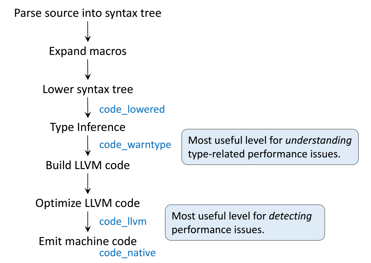
* `Julia`'s efficiency results from its capability to infer the types of **all** variables within a function and then call LLVM compiler to generate optimized machine code at run-time.
Consider the `g` (doubling) function defined earlier. This function will work on **any** type which has a method for `+`.
```{julia}
g(2), g(2.0)
```
**Step 1**: Parse Julia code into [abstract syntax tree (AST)](https://en.wikipedia.org/wiki/Abstract_syntax_tree).
```{julia}
@code_lowered g(2)
```
**Step 2**: Type inference according to input type.
```{julia}
# type inference for integer input
@code_warntype g(2)
```
```{julia}
# type inference for Float64 input
@code_warntype g(2.0)
```
**Step 3**: Compile into **LLVM bitcode** (equivalent of R bytecode generated by the `compiler` package).
```{julia}
# LLVM bitcode for integer input
@code_llvm g(2)
```
```{julia}
# LLVM bitcode for Float64 input
@code_llvm g(2.0)
```
We didn't provide a type annotation. But different LLVM bitcodes were generated depending on the argument type!
In R or Python, `g(2)` and `g(2.0)` would use the same code for both.
In Julia, `g(2)` and `g(2.0)` dispatches to optimized code for `Int64` and `Float64`, respectively.
For integer input `x`, LLVM compiler is smart enough to know `x + x` is simply shifting `x` by 1 bit, which is faster than addition.
* **Step 4**: Lowest level is the **assembly code**, which is machine dependent.
```{julia}
# Assembly code for integer input
@code_native g(2)
```
```{julia}
# Assembly code for Float64 input
@code_native g(2.0)
```
## Profiling Julia code
Julia has several built-in tools for profiling. The `@time` marco outputs run time and heap allocation. Note the first call of a function incurs (substantial) compilation time.
```{julia}
# a function defined earlier
function tally(x::Array)
s = zero(eltype(x))
for v in x
s += v
end
s
end
using Random
Random.seed!(257)
a = rand(20_000_000)
@time tally(a) # first run: include compile time
```
```{julia}
@time tally(a)
```
For more robust benchmarking, the [BenchmarkTools.jl](https://github.com/JuliaCI/BenchmarkTools.jl) package is highly recommended.
```{julia}
@benchmark tally($a)
```
The `Profile` module gives line by line profile results.
```{julia}
Profile.clear()
@profile tally(a)
Profile.print(format=:flat)
```
One can use [`ProfileView`](https://github.com/timholy/ProfileView.jl) package for better visualization of profile data:
```julia
using ProfileView
ProfileView.view()
```
```{julia}
# check type stability
@code_warntype tally(a)
```
```{julia}
# check LLVM bitcode
@code_llvm tally(a)
```
```{julia}
@code_native tally(a)
```
**Exercise:** Annotate the loop in `tally` function by `@simd` and look for the difference in LLVM bitcode and machine code.
## Memory profiling
Detailed memory profiling requires a detour. First let's write a script `bar.jl`, which contains the workload function `tally` and a wrapper for profiling.
```{julia}
;cat bar.jl
```
Next, in terminal, we run the script with `--track-allocation=user` option.
```{julia}
#;julia --track-allocation=user bar.jl
```
The profiler outputs a file `bar.jl.51116.mem`.
```{julia}
;cat bar.jl.51116.mem
```
|
|----------------------------------|------------------------------------|
|||
* `Julia`'s efficiency results from its capability to infer the types of **all** variables within a function and then call LLVM compiler to generate optimized machine code at run-time.
Consider the `g` (doubling) function defined earlier. This function will work on **any** type which has a method for `+`.
```{julia}
g(2), g(2.0)
```
**Step 1**: Parse Julia code into [abstract syntax tree (AST)](https://en.wikipedia.org/wiki/Abstract_syntax_tree).
```{julia}
@code_lowered g(2)
```
**Step 2**: Type inference according to input type.
```{julia}
# type inference for integer input
@code_warntype g(2)
```
```{julia}
# type inference for Float64 input
@code_warntype g(2.0)
```
**Step 3**: Compile into **LLVM bitcode** (equivalent of R bytecode generated by the `compiler` package).
```{julia}
# LLVM bitcode for integer input
@code_llvm g(2)
```
```{julia}
# LLVM bitcode for Float64 input
@code_llvm g(2.0)
```
We didn't provide a type annotation. But different LLVM bitcodes were generated depending on the argument type!
In R or Python, `g(2)` and `g(2.0)` would use the same code for both.
In Julia, `g(2)` and `g(2.0)` dispatches to optimized code for `Int64` and `Float64`, respectively.
For integer input `x`, LLVM compiler is smart enough to know `x + x` is simply shifting `x` by 1 bit, which is faster than addition.
* **Step 4**: Lowest level is the **assembly code**, which is machine dependent.
```{julia}
# Assembly code for integer input
@code_native g(2)
```
```{julia}
# Assembly code for Float64 input
@code_native g(2.0)
```
## Profiling Julia code
Julia has several built-in tools for profiling. The `@time` marco outputs run time and heap allocation. Note the first call of a function incurs (substantial) compilation time.
```{julia}
# a function defined earlier
function tally(x::Array)
s = zero(eltype(x))
for v in x
s += v
end
s
end
using Random
Random.seed!(257)
a = rand(20_000_000)
@time tally(a) # first run: include compile time
```
```{julia}
@time tally(a)
```
For more robust benchmarking, the [BenchmarkTools.jl](https://github.com/JuliaCI/BenchmarkTools.jl) package is highly recommended.
```{julia}
@benchmark tally($a)
```
The `Profile` module gives line by line profile results.
```{julia}
Profile.clear()
@profile tally(a)
Profile.print(format=:flat)
```
One can use [`ProfileView`](https://github.com/timholy/ProfileView.jl) package for better visualization of profile data:
```julia
using ProfileView
ProfileView.view()
```
```{julia}
# check type stability
@code_warntype tally(a)
```
```{julia}
# check LLVM bitcode
@code_llvm tally(a)
```
```{julia}
@code_native tally(a)
```
**Exercise:** Annotate the loop in `tally` function by `@simd` and look for the difference in LLVM bitcode and machine code.
## Memory profiling
Detailed memory profiling requires a detour. First let's write a script `bar.jl`, which contains the workload function `tally` and a wrapper for profiling.
```{julia}
;cat bar.jl
```
Next, in terminal, we run the script with `--track-allocation=user` option.
```{julia}
#;julia --track-allocation=user bar.jl
```
The profiler outputs a file `bar.jl.51116.mem`.
```{julia}
;cat bar.jl.51116.mem
```