---
title: Computer Arithmetics
subtitle: Biostat/Biomath M257
author: Dr. Hua Zhou @ UCLA
date: today
format:
html:
theme: cosmo
embed-resources: true
number-sections: true
toc: true
toc-depth: 4
toc-location: left
code-fold: false
jupyter:
jupytext:
formats: 'ipynb,qmd'
text_representation:
extension: .qmd
format_name: quarto
format_version: '1.0'
jupytext_version: 1.14.5
kernelspec:
display_name: Julia 1.8.5
language: julia
name: julia-1.8
---
System information (for reproducibility):
```{julia}
versioninfo()
```
Load packages:
```{julia}
using Pkg
Pkg.activate(pwd())
Pkg.instantiate()
Pkg.status()
```
## Units of computer storage
* `bit` = `binary` + `digit` (coined by statistician [John Tukey](https://en.wikipedia.org/wiki/Bit#History)).
* `byte` = 8 bits.
* KB = kilobyte = $10^3$ bytes.
* MB = megabytes = $10^6$ bytes.
* GB = gigabytes = $10^9$ bytes. Typical RAM size.
* TB = terabytes = $10^{12}$ bytes. Typical hard drive size. Size of NYSE each trading session.
* PB = petabytes = $10^{15}$ bytes.
* EB = exabytes = $10^{18}$ bytes. Size of all healthcare data in 2011 is ~150 EB.
* ZB = zetabytes = $10^{21}$ bytes.
Difference between `KB` and `KiB`: `1 KB = 1000 bytes` but `1 KiB = 1024 bytes`.
Difference between `TB` and `TiB`: `1 TB = 1000 GB` but `1 TiB = 1024 GB`.
Julia function `Base.summarysize` shows the amount of memory (in bytes) used by an object.
```{julia}
x = rand(100, 100)
Base.summarysize(x)
```
`varinfo()` function prints all variables in workspace and their sizes.
```{julia}
varinfo() # similar to Matlab whos()
```
## Storage of Characters
* Plain text files are stored in the form of characters: `.jl`, `.r`, `.c`, `.cpp`, `.ipynb`, `.html`, `.tex`, ...
* ASCII (American Code for Information Interchange): 7 bits, only $2^7=128$ characters.
```{julia}
# integers 0, 1, ..., 127 and corresponding ascii character
[0:127 Char.(0:127)]
```
* Extended ASCII: 8 bits, $2^8=256$ characters.
```{julia}
# integers 128, 129, ..., 255 and corresponding extended ascii character
# show(STDOUT, "text/plain", [128:255 Char.(128:255)])
[128:255 Char.(128:255)]
```
* Unicode: UTF-8, UTF-16 and UTF-32 support many more characters including foreign characters; last 7 digits conform to ASCII.
* [UTF-8](https://en.wikipedia.org/wiki/UTF-8) is the current dominant character encoding on internet.
 * Julia supports the full range of UTF-8 characters. You can type many Unicode math symbols by typing the backslashed LaTeX symbol name followed by tab.
```{julia}
# \beta-
β = 0.0
# \beta--\hat-
β̂ = 0.0
```
* For a table of unicode symbols that can be entered via tab completion of LaTeX-like abbreviations:
## Integers: fixed-point number system
* Fixed-point number system is a computer model for integers $\mathbb{Z}$.
* The number of bits and method of representing negative numbers vary from system to system.
- The `integer` type in R has $M=32$ or 64 bits, determined by machine word size.
- Matlab has `(u)int8`, `(u)int16`, `(u)int32`, `(u)int64`.
* Julia has even more integer types. Using `Plots.jl` and `GraphRecipes.jl` packages, we can [visualize the type tree](http://www.breloff.com/Graphs/) under `Integer`
- Storage for a `Signed` or `Unsigned` integer can be $M = 8, 16, 32, 64$ or 128 bits.
- GraphRecipes.jl package has a convenience function for plotting the type hiearchy.
```{julia}
using GraphRecipes, Plots
#pyplot(size=(800, 600))
gr()
theme(:default)
plot(Integer, method = :tree, fontsize = 4)
plot!(size = (1200, 800))
```
### Signed integers
* First bit indicates sign.
- `0` for nonnegative numbers
- `1` for negative numbers
* **Two's complement representation** for negative numbers.
- Sign bit is set to 1
- remaining bits are set to opposite values
- 1 is added to the result
- Two's complement representation of a negative integer `x` is same as the unsigned integer `2^64 + x`.
```{julia}
@show typeof(18)
@show bitstring(18)
@show bitstring(-18) # two's complement representation
@show bitstring(UInt64(Int128(2)^64 - 18)) == bitstring(-18) # modular arithmetic
@show bitstring(2 * 18) # shift bits of 18
@show bitstring(2 * -18); # shift bits of -18
```
* Two's complement representation respects modular arithmetic nicely.
Addition of any two signed integers are just bitwise addition, possibly modulo $2^M$
* Julia supports the full range of UTF-8 characters. You can type many Unicode math symbols by typing the backslashed LaTeX symbol name followed by tab.
```{julia}
# \beta-
β = 0.0
# \beta--\hat-
β̂ = 0.0
```
* For a table of unicode symbols that can be entered via tab completion of LaTeX-like abbreviations:
## Integers: fixed-point number system
* Fixed-point number system is a computer model for integers $\mathbb{Z}$.
* The number of bits and method of representing negative numbers vary from system to system.
- The `integer` type in R has $M=32$ or 64 bits, determined by machine word size.
- Matlab has `(u)int8`, `(u)int16`, `(u)int32`, `(u)int64`.
* Julia has even more integer types. Using `Plots.jl` and `GraphRecipes.jl` packages, we can [visualize the type tree](http://www.breloff.com/Graphs/) under `Integer`
- Storage for a `Signed` or `Unsigned` integer can be $M = 8, 16, 32, 64$ or 128 bits.
- GraphRecipes.jl package has a convenience function for plotting the type hiearchy.
```{julia}
using GraphRecipes, Plots
#pyplot(size=(800, 600))
gr()
theme(:default)
plot(Integer, method = :tree, fontsize = 4)
plot!(size = (1200, 800))
```
### Signed integers
* First bit indicates sign.
- `0` for nonnegative numbers
- `1` for negative numbers
* **Two's complement representation** for negative numbers.
- Sign bit is set to 1
- remaining bits are set to opposite values
- 1 is added to the result
- Two's complement representation of a negative integer `x` is same as the unsigned integer `2^64 + x`.
```{julia}
@show typeof(18)
@show bitstring(18)
@show bitstring(-18) # two's complement representation
@show bitstring(UInt64(Int128(2)^64 - 18)) == bitstring(-18) # modular arithmetic
@show bitstring(2 * 18) # shift bits of 18
@show bitstring(2 * -18); # shift bits of -18
```
* Two's complement representation respects modular arithmetic nicely.
Addition of any two signed integers are just bitwise addition, possibly modulo $2^M$
 * Arithmetics (addition, substraction, multiplication) of integers are **exact** except for the possiblity of overflow and underflow.
* **Range** of representable integers by $M$-bit **signed integer** is $[-2^{M-1},2^{M-1}-1]$.
- Julia functions `typemin(T)` and `typemax(T)` give the lowest and highest representable number of a type `T` respectively
```{julia}
typemin(Int64), typemax(Int64)
```
```{julia}
for T in [Int8, Int16, Int32, Int64, Int128]
println(T, '\t', typemin(T), '\t', typemax(T))
end
```
### Unsigned integers
* For unsigned integers, the range is $[0,2^M-1]$.
```{julia}
for t in [UInt8, UInt16, UInt32, UInt64, UInt128]
println(t, '\t', typemin(t), '\t', typemax(t))
end
```
### `BigInt`
Julia `BigInt` type is arbitrary precision.
```{julia}
@show typemax(Int128)
@show typemax(Int128) + 1 # modular arithmetic!
@show BigInt(typemax(Int128)) + 1;
```
### Overflow and underflow for integer arithmetic
R reports `NA` for integer overflow and underflow.
> **Julia outputs the result according to modular arithmetic.**
```{julia}
@show typemax(Int32)
@show typemax(Int32) + Int32(1); # modular arithmetics!
```
```{julia}
using RCall
R"""
.Machine$integer.max
"""
```
```{julia}
R"""
M <- 32
big <- 2^(M - 1) - 1
as.integer(big)
"""
```
```{julia}
R"""
as.integer(big + 1)
"""
```
## Real numbers: floating-number system
Floating-point number system is a computer model for real numbers.
* Most computer systems adopt the [IEEE 754 standard](https://en.wikipedia.org/wiki/IEEE_floating_point), established in 1985, for floating-point arithmetics.
For the history, see an [interview with William Kahan](http://www.cs.berkeley.edu/~wkahan/ieee754status/754story.html).
* In the scientific notation, a real number is represented as
$$\pm d_0.d_1d_2 \cdots d_p \times b^e.$$
In computer, the _base_ is $b=2$ and the digits $d_i$ are 0 or 1.
* **Normalized** vs **denormalized** numbers. For example, decimal number 18 is
$$ +1.0010 \times 2^4 \quad (\text{normalized})$$
or, equivalently,
$$ +0.1001 \times 2^5 \quad (\text{denormalized}).$$
* In the floating-number system, computer stores
- sign bit
- the _fraction_ (or _mantissa_, or _significand_) of the **normalized** representation
- the actual exponent _plus_ a bias
```{julia}
using GraphRecipes, Plots
#pyplot(size=(800, 600))
gr()
theme(:default)
plot(AbstractFloat, method = :tree, fontsize = 4)
plot!(size = (1200, 900))
```
### Double precision (Float64)
* Arithmetics (addition, substraction, multiplication) of integers are **exact** except for the possiblity of overflow and underflow.
* **Range** of representable integers by $M$-bit **signed integer** is $[-2^{M-1},2^{M-1}-1]$.
- Julia functions `typemin(T)` and `typemax(T)` give the lowest and highest representable number of a type `T` respectively
```{julia}
typemin(Int64), typemax(Int64)
```
```{julia}
for T in [Int8, Int16, Int32, Int64, Int128]
println(T, '\t', typemin(T), '\t', typemax(T))
end
```
### Unsigned integers
* For unsigned integers, the range is $[0,2^M-1]$.
```{julia}
for t in [UInt8, UInt16, UInt32, UInt64, UInt128]
println(t, '\t', typemin(t), '\t', typemax(t))
end
```
### `BigInt`
Julia `BigInt` type is arbitrary precision.
```{julia}
@show typemax(Int128)
@show typemax(Int128) + 1 # modular arithmetic!
@show BigInt(typemax(Int128)) + 1;
```
### Overflow and underflow for integer arithmetic
R reports `NA` for integer overflow and underflow.
> **Julia outputs the result according to modular arithmetic.**
```{julia}
@show typemax(Int32)
@show typemax(Int32) + Int32(1); # modular arithmetics!
```
```{julia}
using RCall
R"""
.Machine$integer.max
"""
```
```{julia}
R"""
M <- 32
big <- 2^(M - 1) - 1
as.integer(big)
"""
```
```{julia}
R"""
as.integer(big + 1)
"""
```
## Real numbers: floating-number system
Floating-point number system is a computer model for real numbers.
* Most computer systems adopt the [IEEE 754 standard](https://en.wikipedia.org/wiki/IEEE_floating_point), established in 1985, for floating-point arithmetics.
For the history, see an [interview with William Kahan](http://www.cs.berkeley.edu/~wkahan/ieee754status/754story.html).
* In the scientific notation, a real number is represented as
$$\pm d_0.d_1d_2 \cdots d_p \times b^e.$$
In computer, the _base_ is $b=2$ and the digits $d_i$ are 0 or 1.
* **Normalized** vs **denormalized** numbers. For example, decimal number 18 is
$$ +1.0010 \times 2^4 \quad (\text{normalized})$$
or, equivalently,
$$ +0.1001 \times 2^5 \quad (\text{denormalized}).$$
* In the floating-number system, computer stores
- sign bit
- the _fraction_ (or _mantissa_, or _significand_) of the **normalized** representation
- the actual exponent _plus_ a bias
```{julia}
using GraphRecipes, Plots
#pyplot(size=(800, 600))
gr()
theme(:default)
plot(AbstractFloat, method = :tree, fontsize = 4)
plot!(size = (1200, 900))
```
### Double precision (Float64)
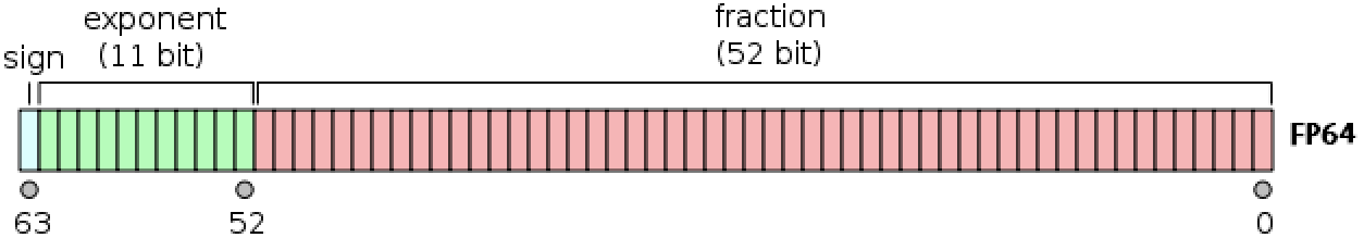 - Double precision (64 bits = 8 bytes) numbers are the dominant data type in scientific computing.
- In Julia, `Float64` is the type for double precision numbers.
- First bit is sign bit.
- $p=52$ significant bits.
- 11 exponent bits: $e_{\max}=1023$, $e_{\min}=-1022$, **bias**=1023.
- $e_{\text{min}}-1$ and $e_{\text{max}}+1$ are reserved for special numbers.
- range of **magnitude**: $10^{\pm 308}$ in decimal because $\log_{10} (2^{1023}) \approx 308$.
- **precision** to the $- \log_{10}(2^{-52}) \approx 15$ decimal point.
```{julia}
println("Double precision:")
@show bitstring(Float64(18)) # 18 in double precision
@show bitstring(Float64(-18)); # -18 in double precision
```
### Single precision (Float32)
- Double precision (64 bits = 8 bytes) numbers are the dominant data type in scientific computing.
- In Julia, `Float64` is the type for double precision numbers.
- First bit is sign bit.
- $p=52$ significant bits.
- 11 exponent bits: $e_{\max}=1023$, $e_{\min}=-1022$, **bias**=1023.
- $e_{\text{min}}-1$ and $e_{\text{max}}+1$ are reserved for special numbers.
- range of **magnitude**: $10^{\pm 308}$ in decimal because $\log_{10} (2^{1023}) \approx 308$.
- **precision** to the $- \log_{10}(2^{-52}) \approx 15$ decimal point.
```{julia}
println("Double precision:")
@show bitstring(Float64(18)) # 18 in double precision
@show bitstring(Float64(-18)); # -18 in double precision
```
### Single precision (Float32)
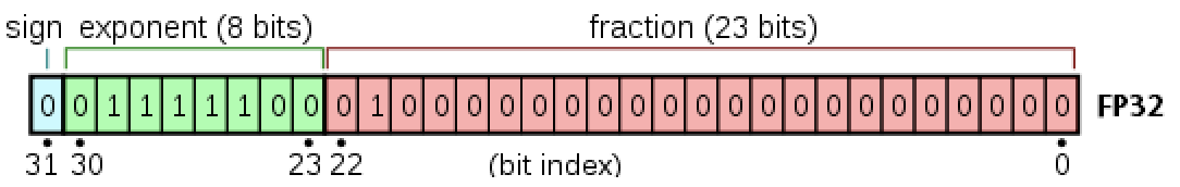 - In Julia, `Float32` is the type for single precision numbers.
- First bit is sign bit.
- $p=23$ significant bits.
- 8 exponent bits: $e_{\max}=127$, $e_{\min}=-126$, **bias**=127.
- $e_{\text{min}}-1$ and $e_{\text{max}}+1$ are reserved for special numbers.
- range of **magnitude**: $10^{\pm 38}$ in decimal because $\log_{10} (2^{127}) \approx 38$.
- **precision**: $- \log_{10}(2^{-23}) \approx 7$ decimal point.
```{julia}
println("Single precision:")
@show bitstring(Float32(18.0)) # 18 in single precision
@show bitstring(Float32(-18.0)); # -18 in single precision
```
### Half precision (Float16)
- In Julia, `Float32` is the type for single precision numbers.
- First bit is sign bit.
- $p=23$ significant bits.
- 8 exponent bits: $e_{\max}=127$, $e_{\min}=-126$, **bias**=127.
- $e_{\text{min}}-1$ and $e_{\text{max}}+1$ are reserved for special numbers.
- range of **magnitude**: $10^{\pm 38}$ in decimal because $\log_{10} (2^{127}) \approx 38$.
- **precision**: $- \log_{10}(2^{-23}) \approx 7$ decimal point.
```{julia}
println("Single precision:")
@show bitstring(Float32(18.0)) # 18 in single precision
@show bitstring(Float32(-18.0)); # -18 in single precision
```
### Half precision (Float16)
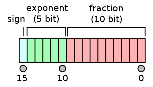 - In Julia, `Float16` is the type for half precision numbers.
- First bit is sign bit.
- $p=10$ significant bits.
- 5 exponent bits: $e_{\max}=15$, $e_{\min}=-14$, bias=15.
- $e_{\text{min}}-1$ and $e_{\text{max}}+1$ are reserved for special numbers.
- range of **magnitude**: $10^{\pm 4}$ in decimal because $\log_{10} (2^{15}) \approx 4$.
- **precision**: $\log_{10}(2^{10}) \approx 3$ decimal point.
```{julia}
println("Half precision:")
@show bitstring(Float16(18)) # 18 in half precision
@show bitstring(Float16(-18)); # -18 in half precision
```
### Special floating-point numbers.
- Exponent $e_{\max}+1$ (exponent bits all 1) plus a zero mantissa means $\pm \infty$.
```{julia}
@show bitstring(Inf) # Inf in double precision
@show bitstring(-Inf); # -Inf in double precision
```
- Exponent $e_{\max}+1$ (exponent bits all 1) plus a nonzero mantissa means `NaN`. `NaN` could be produced from `0 / 0`, `0 * Inf`, ...
- In general `NaN ≠ NaN` bitwise. Test whether a number is `NaN` by `isnan` function.
```{julia}
@show bitstring(0 / 0) # NaN
@show bitstring(0 * Inf); # NaN
```
- Exponent $e_{\min}-1$ (exponent bits all 0) with a zero mantissa represents the real number 0.
```{julia}
@show bitstring(0.0) # +0 in double precision
@show bitstring(-0.0); # -0 in double precision
```
There are some special rules in IEEE 754 for [signed zeros](https://en.wikipedia.org/wiki/Signed_zero).
- Exponent $e_{\min}-1$ (exponent bits all 0) with a nonzero mantissa are for numbers less than $b^{e_{\min}}$.
Numbers are _denormalized_ in the range $(0,b^{e_{\min}})$ -- **graceful underflow**.
```{julia}
@show nextfloat(0.0) # next representable number
@show bitstring(nextfloat(0.0)); # denormalized
```
### Rounding
* Rounding is necessary whenever a number has more than $p$ significand bits. Most computer systems use the default IEEE 754 **round to nearest** mode (also called **ties to even** mode). Julia offers several [rounding modes](https://docs.julialang.org/en/v1/base/math/#Base.Rounding.RoundingMode), the default being [`RoundNearest`](https://docs.julialang.org/en/v1/base/math/#Base.Rounding.RoundNearest). For example, the number 0.1 in decimal system cannot be represented accurately as a floating point number:
$$ 0.1 = 1.\underbrace{1001}_\text{repeat}\underbrace{1001}... \times 2^{-4} $$
```{julia}
# half precision Float16, ...110(011...) rounds down to 110
@show bitstring(Float16(0.1))
# single precision Float32, ...100(110...) rounds up to 101
@show bitstring(0.1f0)
# double precision Float64, ...001(100..) rounds up to 010
@show bitstring(0.1);
```
For a number with mantissa ending with ...001(100..., all 0 digits after), it's a tie and will be rounded to ...010 to make the mantissa even.
### Summary
- **Double precision**: range $\pm 10^{\pm 308}$ with precision up to 16 decimal digits.
- **Single precision**: range $\pm 10^{\pm 38}$ with precision up to 7 decimal digits.
- **Half precision**: range $\pm 10^{\pm 4}$ with precision up to 3 decimal digits.
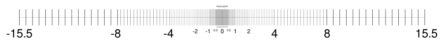
- The floating-point numbers do not occur uniformly over the real number line. Each magnitude has same number of representible numbers, except those around 0 (graceful underflow).
- In Julia, `Float16` is the type for half precision numbers.
- First bit is sign bit.
- $p=10$ significant bits.
- 5 exponent bits: $e_{\max}=15$, $e_{\min}=-14$, bias=15.
- $e_{\text{min}}-1$ and $e_{\text{max}}+1$ are reserved for special numbers.
- range of **magnitude**: $10^{\pm 4}$ in decimal because $\log_{10} (2^{15}) \approx 4$.
- **precision**: $\log_{10}(2^{10}) \approx 3$ decimal point.
```{julia}
println("Half precision:")
@show bitstring(Float16(18)) # 18 in half precision
@show bitstring(Float16(-18)); # -18 in half precision
```
### Special floating-point numbers.
- Exponent $e_{\max}+1$ (exponent bits all 1) plus a zero mantissa means $\pm \infty$.
```{julia}
@show bitstring(Inf) # Inf in double precision
@show bitstring(-Inf); # -Inf in double precision
```
- Exponent $e_{\max}+1$ (exponent bits all 1) plus a nonzero mantissa means `NaN`. `NaN` could be produced from `0 / 0`, `0 * Inf`, ...
- In general `NaN ≠ NaN` bitwise. Test whether a number is `NaN` by `isnan` function.
```{julia}
@show bitstring(0 / 0) # NaN
@show bitstring(0 * Inf); # NaN
```
- Exponent $e_{\min}-1$ (exponent bits all 0) with a zero mantissa represents the real number 0.
```{julia}
@show bitstring(0.0) # +0 in double precision
@show bitstring(-0.0); # -0 in double precision
```
There are some special rules in IEEE 754 for [signed zeros](https://en.wikipedia.org/wiki/Signed_zero).
- Exponent $e_{\min}-1$ (exponent bits all 0) with a nonzero mantissa are for numbers less than $b^{e_{\min}}$.
Numbers are _denormalized_ in the range $(0,b^{e_{\min}})$ -- **graceful underflow**.
```{julia}
@show nextfloat(0.0) # next representable number
@show bitstring(nextfloat(0.0)); # denormalized
```
### Rounding
* Rounding is necessary whenever a number has more than $p$ significand bits. Most computer systems use the default IEEE 754 **round to nearest** mode (also called **ties to even** mode). Julia offers several [rounding modes](https://docs.julialang.org/en/v1/base/math/#Base.Rounding.RoundingMode), the default being [`RoundNearest`](https://docs.julialang.org/en/v1/base/math/#Base.Rounding.RoundNearest). For example, the number 0.1 in decimal system cannot be represented accurately as a floating point number:
$$ 0.1 = 1.\underbrace{1001}_\text{repeat}\underbrace{1001}... \times 2^{-4} $$
```{julia}
# half precision Float16, ...110(011...) rounds down to 110
@show bitstring(Float16(0.1))
# single precision Float32, ...100(110...) rounds up to 101
@show bitstring(0.1f0)
# double precision Float64, ...001(100..) rounds up to 010
@show bitstring(0.1);
```
For a number with mantissa ending with ...001(100..., all 0 digits after), it's a tie and will be rounded to ...010 to make the mantissa even.
### Summary
- **Double precision**: range $\pm 10^{\pm 308}$ with precision up to 16 decimal digits.
- **Single precision**: range $\pm 10^{\pm 38}$ with precision up to 7 decimal digits.
- **Half precision**: range $\pm 10^{\pm 4}$ with precision up to 3 decimal digits.
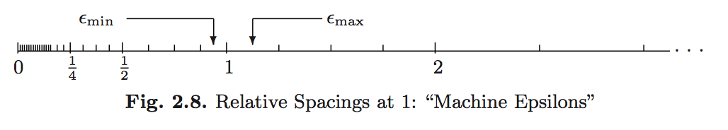
- The floating-point numbers do not occur uniformly over the real number line. Each magnitude has same number of representible numbers, except those around 0 (graceful underflow).
 - **Machine epsilons** are the spacings of numbers around 1:
$$\epsilon_{\min}=b^{-p}, \quad \epsilon_{\max} = b^{1-p}.$$
- **Machine epsilons** are the spacings of numbers around 1:
$$\epsilon_{\min}=b^{-p}, \quad \epsilon_{\max} = b^{1-p}.$$
 ```{julia}
@show eps(Float32) # machine epsilon for a floating point type
@show eps(Float64) # same as eps()
# eps(x) is the spacing after x
@show eps(100.0)
@show eps(0.0) # grace underflow
# nextfloat(x) and prevfloat(x) give the neighbors of x
@show x = 1.25f0
@show prevfloat(x), x, nextfloat(x)
@show bitstring(prevfloat(x)), bitstring(x), bitstring(nextfloat(x));
```
* In R, the variable `.Machine` contains numerical characteristics of the machine.
```{julia}
R"""
.Machine
"""
```
* Julia provides `Float16` (half precision), `Float32` (single precision), `Float64` (double precision), and `BigFloat` (arbitrary precision).
### Overflow and underflow of floating-point number
* For double precision, the range is $\pm 10^{\pm 308}$. In most situations, underflow (magnitude of result is less than $10^{-308}$) is preferred over overflow (magnitude of result is larger than $10^{308}$). Overflow produces $\pm \inf$. Underflow yields zeros or denormalized numbers.
* E.g., the logit link function is
$$p(x) = \frac{\exp (x^T \beta)}{1 + \exp (x^T \beta)} = \frac{1}{1+\exp(- x^T \beta)}.$$
The former expression can easily lead to `Inf / Inf = NaN`, while the latter expression leads to graceful underflow.
* `floatmin` and `floatmax` functions gives largest and smallest _finite_ number represented by a type.
```{julia}
for T in [Float16, Float32, Float64]
println(
T, '\t',
floatmin(T), '\t',
floatmax(T), '\t',
typemin(T), '\t',
typemax(T), '\t',
eps(T)
)
end
```
### Arbitrary precision
* `BigFloat` in Julia offers arbitrary precision.
```{julia}
@show precision(BigFloat) # default precision (how many bits) of BigFloat
@show floatmin(BigFloat)
@show floatmax(BigFloat);
```
```{julia}
@show BigFloat(π); # default precision for BigFloat is 256 bits
# set precision to 1024 bits
setprecision(BigFloat, 1024) do
@show BigFloat(π)
end;
```
## Catastrophic cancellation
* **Scenario 1**: Addition or subtraction of two numbers of widely different magnitudes: $a+b$ or $a-b$ where $a \gg b$ or $a \ll b$. We loose the precision in the number of smaller magnitude. Consider
$$\begin{eqnarray*}
a &=& x.xxx ... \times 2^{30} \\
b &=& y.yyy... \times 2^{-30}
\end{eqnarray*}$$
What happens when computer calculates $a+b$? We get $a+b=a$!
```{julia}
@show a = 2.0^30
@show b = 2.0^-30
@show a + b == a
```
* **Scenario 2**: Subtraction of two nearly equal numbers eliminates significant digits. $a-b$ where $a \approx b$. Consider
$$\begin{eqnarray*}
a &=& x.xxxxxxxxxx1ssss \\
b &=& x.xxxxxxxxxx0tttt
\end{eqnarray*}$$
The result is $1.vvvvu...u$ where $u$ are unassigned digits.
```{julia}
a = 1.2345678f0 # rounding
@show bitstring(a) # rounding
b = 1.2345677f0
@show bitstring(b)
# correct result should be 1e-7
# we see big error due to catastrophic cancellation
@show a - b
```
* Implications for numerical computation
- Rule 1: add small numbers together before adding larger ones
- Rule 2: add numbers of like magnitude together (paring). When all numbers are of same sign and similar magnitude, add in pairs so each stage the summands are of similar magnitude
- Rule 3: avoid substraction of two numbers that are nearly equal
### Algebraic laws
Floating-point numbers may violate many algebraic laws we are familiar with, such as the associative and distributive laws. See Homework 1 problems.
## Further reading
* Textbook treatment, e.g., Chapter II.2 of [Computational Statistics](http://ucla.worldcat.org/title/computational-statistics/oclc/437345409&referer=brief_results) by James Gentle (2010).
* [What every computer scientist should know about floating-point arithmetic](https://ucla-biostat-257.github.io/2023spring/readings/Goldberg91FloatingPoint.pdf) by David Goldberg (1991).
```{julia}
@show eps(Float32) # machine epsilon for a floating point type
@show eps(Float64) # same as eps()
# eps(x) is the spacing after x
@show eps(100.0)
@show eps(0.0) # grace underflow
# nextfloat(x) and prevfloat(x) give the neighbors of x
@show x = 1.25f0
@show prevfloat(x), x, nextfloat(x)
@show bitstring(prevfloat(x)), bitstring(x), bitstring(nextfloat(x));
```
* In R, the variable `.Machine` contains numerical characteristics of the machine.
```{julia}
R"""
.Machine
"""
```
* Julia provides `Float16` (half precision), `Float32` (single precision), `Float64` (double precision), and `BigFloat` (arbitrary precision).
### Overflow and underflow of floating-point number
* For double precision, the range is $\pm 10^{\pm 308}$. In most situations, underflow (magnitude of result is less than $10^{-308}$) is preferred over overflow (magnitude of result is larger than $10^{308}$). Overflow produces $\pm \inf$. Underflow yields zeros or denormalized numbers.
* E.g., the logit link function is
$$p(x) = \frac{\exp (x^T \beta)}{1 + \exp (x^T \beta)} = \frac{1}{1+\exp(- x^T \beta)}.$$
The former expression can easily lead to `Inf / Inf = NaN`, while the latter expression leads to graceful underflow.
* `floatmin` and `floatmax` functions gives largest and smallest _finite_ number represented by a type.
```{julia}
for T in [Float16, Float32, Float64]
println(
T, '\t',
floatmin(T), '\t',
floatmax(T), '\t',
typemin(T), '\t',
typemax(T), '\t',
eps(T)
)
end
```
### Arbitrary precision
* `BigFloat` in Julia offers arbitrary precision.
```{julia}
@show precision(BigFloat) # default precision (how many bits) of BigFloat
@show floatmin(BigFloat)
@show floatmax(BigFloat);
```
```{julia}
@show BigFloat(π); # default precision for BigFloat is 256 bits
# set precision to 1024 bits
setprecision(BigFloat, 1024) do
@show BigFloat(π)
end;
```
## Catastrophic cancellation
* **Scenario 1**: Addition or subtraction of two numbers of widely different magnitudes: $a+b$ or $a-b$ where $a \gg b$ or $a \ll b$. We loose the precision in the number of smaller magnitude. Consider
$$\begin{eqnarray*}
a &=& x.xxx ... \times 2^{30} \\
b &=& y.yyy... \times 2^{-30}
\end{eqnarray*}$$
What happens when computer calculates $a+b$? We get $a+b=a$!
```{julia}
@show a = 2.0^30
@show b = 2.0^-30
@show a + b == a
```
* **Scenario 2**: Subtraction of two nearly equal numbers eliminates significant digits. $a-b$ where $a \approx b$. Consider
$$\begin{eqnarray*}
a &=& x.xxxxxxxxxx1ssss \\
b &=& x.xxxxxxxxxx0tttt
\end{eqnarray*}$$
The result is $1.vvvvu...u$ where $u$ are unassigned digits.
```{julia}
a = 1.2345678f0 # rounding
@show bitstring(a) # rounding
b = 1.2345677f0
@show bitstring(b)
# correct result should be 1e-7
# we see big error due to catastrophic cancellation
@show a - b
```
* Implications for numerical computation
- Rule 1: add small numbers together before adding larger ones
- Rule 2: add numbers of like magnitude together (paring). When all numbers are of same sign and similar magnitude, add in pairs so each stage the summands are of similar magnitude
- Rule 3: avoid substraction of two numbers that are nearly equal
### Algebraic laws
Floating-point numbers may violate many algebraic laws we are familiar with, such as the associative and distributive laws. See Homework 1 problems.
## Further reading
* Textbook treatment, e.g., Chapter II.2 of [Computational Statistics](http://ucla.worldcat.org/title/computational-statistics/oclc/437345409&referer=brief_results) by James Gentle (2010).
* [What every computer scientist should know about floating-point arithmetic](https://ucla-biostat-257.github.io/2023spring/readings/Goldberg91FloatingPoint.pdf) by David Goldberg (1991).