---
title: Numerical Linear Algebra
subtitle: Biostat/Biomath M257
author: Dr. Hua Zhou @ UCLA
date: today
format:
html:
theme: cosmo
embed-resources: true
number-sections: true
toc: true
toc-depth: 4
toc-location: left
code-fold: false
jupyter:
jupytext:
formats: 'ipynb,qmd'
text_representation:
extension: .qmd
format_name: quarto
format_version: '1.0'
jupytext_version: 1.14.5
kernelspec:
display_name: Julia (8 threads) 1.8.5
language: julia
name: julia-_8-threads_-1.8
---
System information (for reproducibility):
```{julia}
versioninfo()
```
Load packages:
```{julia}
using Pkg
Pkg.activate(pwd())
Pkg.instantiate()
Pkg.status()
```
## Introduction
* Topics in numerical algebra:
- BLAS
- solve linear equations $\mathbf{A} \mathbf{x} = \mathbf{b}$
- regression computations $\mathbf{X}^T \mathbf{X} \beta = \mathbf{X}^T \mathbf{y}$
- eigen-problems $\mathbf{A} \mathbf{x} = \lambda \mathbf{x}$
- generalized eigen-problems $\mathbf{A} \mathbf{x} = \lambda \mathbf{B} \mathbf{x}$
- singular value decompositions $\mathbf{A} = \mathbf{U} \Sigma \mathbf{V}^T$
- iterative methods for numerical linear algebra
* Except for the iterative methods, most of these numerical linear algebra tasks are implemented in the **BLAS** and **LAPACK** libraries. They form the **building blocks** of most statistical computing tasks (optimization, MCMC).
* Our major **goal** (or learning objectives) is to
1. know the complexity (flop count) of each task
2. be familiar with the BLAS and LAPACK functions (what they do)
3. do **not** re-invent wheels by implementing these dense linear algebra subroutines by yourself
4. understand the need for iterative methods
5. apply appropriate numerical algebra tools to various statistical problems
* All high-level languages (Julia, Matlab, Python, R) call BLAS and LAPACK for numerical linear algebra.
- Julia offers more flexibility by exposing interfaces to many BLAS/LAPACK subroutines directly. See [documentation](https://docs.julialang.org/en/v1/stdlib/LinearAlgebra/#BLAS-functions-1).
## BLAS
* BLAS stands for _basic linear algebra subprograms_.
* See [netlib](http://www.netlib.org/blas/) for a complete list of standardized BLAS functions.
* There are many implementations of BLAS.
- [Netlib](http://www.netlib.org/blas/) provides a reference implementation.
- Matlab uses Intel's [MKL](https://www.intel.com/content/www/us/en/docs/oneapi/programming-guide/2023-0/intel-oneapi-math-kernel-library-onemkl.html) (mathematical kernel libaries). **MKL implementation is the gold standard on market.** It is not open source but the compiled library is free for Linux and MacOS. However, not surprisingly, it only works on Intel CPUs.
- Julia uses [OpenBLAS](https://github.com/xianyi/OpenBLAS). **OpenBLAS is the best cross-platform, open source implementation**. With the [MKL.jl](https://github.com/JuliaLinearAlgebra/MKL.jl) package, it's also very easy to use MKL in Julia.
* There are 3 levels of BLAS functions.
- [Level 1](http://www.netlib.org/blas/#_level_1): vector-vector operation
- [Level 2](http://www.netlib.org/blas/#_level_2): matrix-vector operation
- [Level 3](http://www.netlib.org/blas/#_level_3): matrix-matrix operation
| Level | Example Operation | Name | Dimension | Flops |
|-------|----------------------------------------|-------------|-------------------------------------------|-------|
| 1 | $\alpha \gets \mathbf{x}^T \mathbf{y}$ | dot product | $\mathbf{x}, \mathbf{y} \in \mathbb{R}^n$ | $2n$ |
| 1 | $\mathbf{y} \gets \mathbf{y} + \alpha \mathbf{x}$ | axpy | $\alpha \in \mathbb{R}$, $\mathbf{x}, \mathbf{y} \in \mathbb{R}^n$ | $2n$ |
| 2 | $\mathbf{y} \gets \mathbf{y} + \mathbf{A} \mathbf{x}$ | gaxpy | $\mathbf{A} \in \mathbb{R}^{m \times n}$, $\mathbf{x} \in \mathbb{R}^n$, $\mathbf{y} \in \mathbb{R}^m$ | $2mn$ |
| 2 | $\mathbf{A} \gets \mathbf{A} + \mathbf{y} \mathbf{x}^T$ | rank one update | $\mathbf{A} \in \mathbb{R}^{m \times n}$, $\mathbf{x} \in \mathbb{R}^n$, $\mathbf{y} \in \mathbb{R}^m$ | $2mn$ |
| 3 | $\mathbf{C} \gets \mathbf{C} + \mathbf{A} \mathbf{B}$ | matrix multiplication | $\mathbf{A} \in \mathbb{R}^{m \times p}$, $\mathbf{B} \in \mathbb{R}^{p \times n}$, $\mathbf{C} \in \mathbb{R}^{m \times n}$ | $2mnp$ |
* Typical BLAS functions support single precision (S), double precision (D), complex (C), and double complex (Z).
## Examples
> **The form of a mathematical expression and the way the expression should be evaluated in actual practice may be quite different.**
Some operations _appear_ as level-3 but indeed are level-2.
**Example 1**. A common operation in statistics is column scaling or row scaling
$$
\begin{eqnarray*}
\mathbf{A} &=& \mathbf{A} \mathbf{D} \quad \text{(column scaling)} \\
\mathbf{A} &=& \mathbf{D} \mathbf{A} \quad \text{(row scaling)},
\end{eqnarray*}
$$
where $\mathbf{D}$ is diagonal. For example, in generalized linear models (GLMs), the Fisher information matrix takes the form
$$
\mathbf{X}^T \mathbf{W} \mathbf{X},
$$
where $\mathbf{W}$ is a diagonal matrix with observation weights on diagonal.
Column and row scalings are essentially level-2 operations!
```{julia}
using BenchmarkTools, LinearAlgebra, Random
Random.seed!(257) # seed
n = 2000
A = rand(n, n) # n-by-n matrix
d = rand(n) # n vector
D = Diagonal(d) # diagonal matrix with d as diagonal
```
```{julia}
Dfull = diagm(d) # convert to full matrix
```
```{julia}
# this is calling BLAS routine for matrix multiplication: O(n^3) flops
# this is SLOW!
@benchmark $A * $Dfull
```
```{julia}
# dispatch to special method for diagonal matrix multiplication.
# columnwise scaling: O(n^2) flops
@benchmark $A * $D
```
```{julia}
# Or we can use broadcasting (with recycling)
@benchmark $A .* transpose($d)
```
```{julia}
# in-place: avoid allocate space for result
# rmul!: compute matrix-matrix product A*B, overwriting A, and return the result.
@benchmark rmul!($A, $D)
```
```{julia}
# In-place broadcasting
@benchmark $A .= $A .* transpose($d)
```
**Exercise**: Try `@turbo` (SIMD) and `@tturbo` (SIMD) from LoopVectorization.jl package.
**Note:** In R or Matlab, `diag(d)` will create a full matrix. Be cautious using `diag` function: do we really need a full diagonal matrix?
```{julia}
using RCall
R"""
d <- runif(5)
diag(d)
"""
```
```{julia}
#| eval: false
# This works only when Matlab is installed
using MATLAB
mat"""
d = rand(5, 1)
diag(d)
"""
```
**Example 2**. Innter product between two matrices $\mathbf{A}, \mathbf{B} \in \mathbb{R}^{m \times n}$ is often written as
$$
\text{trace}(\mathbf{A}^T \mathbf{B}), \text{trace}(\mathbf{B} \mathbf{A}^T), \text{trace}(\mathbf{A} \mathbf{B}^T), \text{ or } \text{trace}(\mathbf{B}^T \mathbf{A}).
$$
They appear as level-3 operation (matrix multiplication with $O(m^2n)$ or $O(mn^2)$ flops).
```{julia}
Random.seed!(123)
n = 2000
A, B = randn(n, n), randn(n, n)
# slow way to evaluate tr(A'B): 2mn^2 flops
@benchmark tr(transpose($A) * $B)
```
But $\text{trace}(\mathbf{A}^T \mathbf{B}) = <\text{vec}(\mathbf{A}), \text{vec}(\mathbf{B})>$. The latter is level-1 BLAS operation with $O(mn)$ flops.
```{julia}
# smarter way to evaluate tr(A'B): 2mn flops
@benchmark dot($A, $B)
```
**Example 3**. Similarly $\text{diag}(\mathbf{A}^T \mathbf{B})$ can be calculated in $O(mn)$ flops.
```{julia}
# slow way to evaluate diag(A'B): O(n^3)
@benchmark diag(transpose($A) * $B)
```
```{julia}
# smarter way to evaluate diag(A'B): O(n^2)
@benchmark Diagonal(vec(sum($A .* $B, dims = 1)))
```
To get rid of allocation of intermediate arrays at all, we can just write a double loop or use `dot` function.
```{julia}
function diag_matmul!(d, A, B)
m, n = size(A)
@assert size(B) == (m, n) "A and B should have same size"
fill!(d, 0)
for j in 1:n, i in 1:m
d[j] += A[i, j] * B[i, j]
end
Diagonal(d)
end
d = zeros(eltype(A), size(A, 2))
@benchmark diag_matmul!($d, $A, $B)
```
**Exercise**: Try `@turbo` (SIMD) and `@tturbo` (SIMD) from LoopVectorization.jl package.
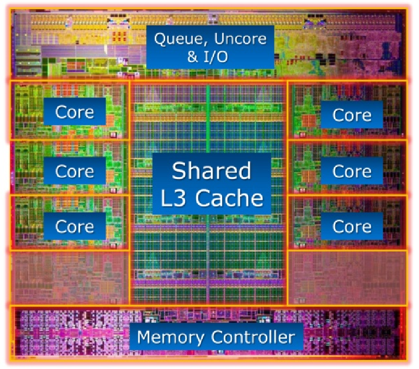
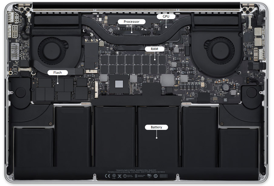
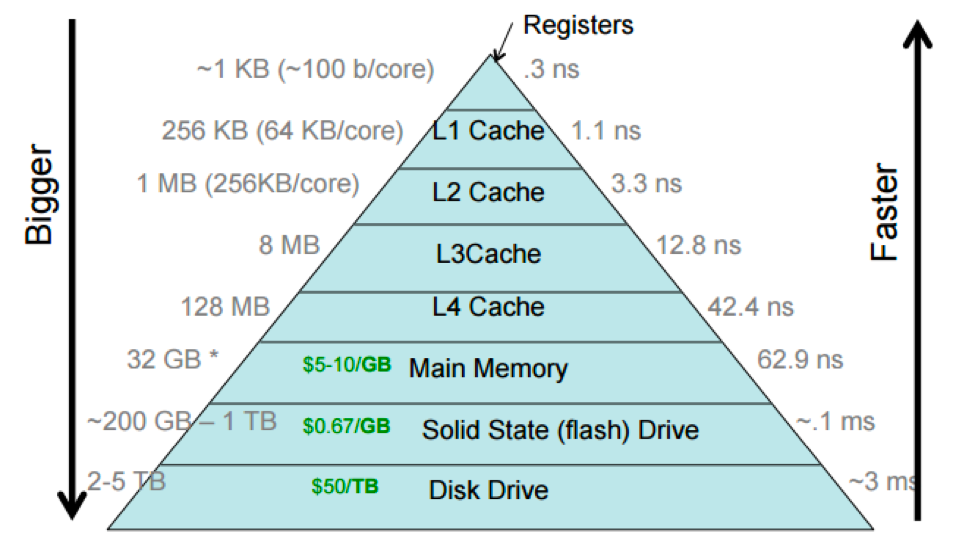
## Memory hierarchy and level-3 fraction
> **Key to high performance is effective use of memory hierarchy. True on all architectures.**
* Flop count is not the sole determinant of algorithm efficiency. Another important factor is data movement through the memory hierarchy.
 Source:
- In Julia, we can query the CPU topology by the `Hwloc.jl` package. For example, this laptop runs an Apple M2 Max chip with 4 efficiency cores and 8 performance cores.
```{julia}
using Hwloc
topology_graphical()
```
* For example, Xeon X5650 CPU has a theoretical throughput of 128 DP GFLOPS but a max memory bandwidth of 32GB/s.
* Can we keep CPU cores busy with enough deliveries of matrix data and ship the results to memory fast enough to avoid backlog?
Answer: use **high-level BLAS** as much as possible.
| BLAS | Dimension | Mem. Refs. | Flops | Ratio |
|--------------------------------|------------------------------------------------------------|------------|--------|-------|
| Level 1: $\mathbf{y} \gets \mathbf{y} + \alpha \mathbf{x}$ | $\mathbf{x}, \mathbf{y} \in \mathbb{R}^n$ | $3n$ | $2n$ | 3:2 |
| Level 2: $\mathbf{y} \gets \mathbf{y} + \mathbf{A} \mathbf{x}$ | $\mathbf{x}, \mathbf{y} \in \mathbb{R}^n$, $\mathbf{A} \in \mathbb{R}^{n \times n}$ | $n^2$ | $2n^2$ | 1:2 |
| Level 3: $\mathbf{C} \gets \mathbf{C} + \mathbf{A} \mathbf{B}$ | $\mathbf{A}, \mathbf{B}, \mathbf{C} \in\mathbb{R}^{n \times n}$ | $4n^2$ | $2n^3$ | 2:n |
* Higher level BLAS (3 or 2) make more effective use of arithmetic logic units (ALU) by keeping them busy. **Surface-to-volume** effect.
Source:
- In Julia, we can query the CPU topology by the `Hwloc.jl` package. For example, this laptop runs an Apple M2 Max chip with 4 efficiency cores and 8 performance cores.
```{julia}
using Hwloc
topology_graphical()
```
* For example, Xeon X5650 CPU has a theoretical throughput of 128 DP GFLOPS but a max memory bandwidth of 32GB/s.
* Can we keep CPU cores busy with enough deliveries of matrix data and ship the results to memory fast enough to avoid backlog?
Answer: use **high-level BLAS** as much as possible.
| BLAS | Dimension | Mem. Refs. | Flops | Ratio |
|--------------------------------|------------------------------------------------------------|------------|--------|-------|
| Level 1: $\mathbf{y} \gets \mathbf{y} + \alpha \mathbf{x}$ | $\mathbf{x}, \mathbf{y} \in \mathbb{R}^n$ | $3n$ | $2n$ | 3:2 |
| Level 2: $\mathbf{y} \gets \mathbf{y} + \mathbf{A} \mathbf{x}$ | $\mathbf{x}, \mathbf{y} \in \mathbb{R}^n$, $\mathbf{A} \in \mathbb{R}^{n \times n}$ | $n^2$ | $2n^2$ | 1:2 |
| Level 3: $\mathbf{C} \gets \mathbf{C} + \mathbf{A} \mathbf{B}$ | $\mathbf{A}, \mathbf{B}, \mathbf{C} \in\mathbb{R}^{n \times n}$ | $4n^2$ | $2n^3$ | 2:n |
* Higher level BLAS (3 or 2) make more effective use of arithmetic logic units (ALU) by keeping them busy. **Surface-to-volume** effect.
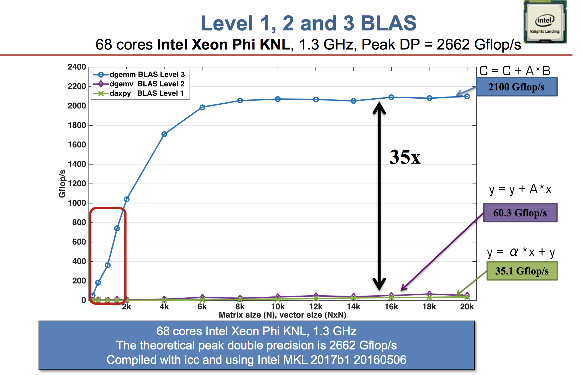 Source: [Jack Dongarra's slides](https://raw.githubusercontent.com/ucla-biostat-257/2023spring/master/readings/SAMSI-0217_Dongarra.pdf).
* A distinction between LAPACK and LINPACK (older version of R uses LINPACK) is that LAPACK makes use of higher level BLAS as much as possible (usually by smart partitioning) to increase the so-called **level-3 fraction**.
* To appreciate the efforts in an optimized BLAS implementation such as OpenBLAS (evolved from GotoBLAS), see the [Quora question](https://www.quora.com/What-algorithm-does-BLAS-use-for-matrix-multiplication-Of-all-the-considerations-e-g-cache-popular-instruction-sets-Big-O-etc-which-one-turned-out-to-be-the-primary-bottleneck), especially the [video](https://youtu.be/JzNpKDW07rw). Bottomline is
> **Get familiar with (good implementations of) BLAS/LAPACK and use them as much as possible.**
## Effect of data layout
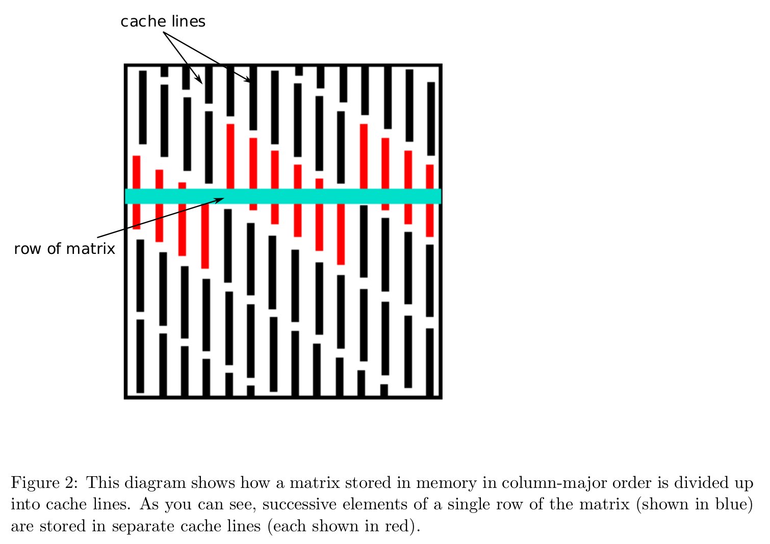
* Data layout in memory affects algorithmic efficiency too. It is much faster to move chunks of data in memory than retrieving/writing scattered data.
* Storage mode: **column-major** (Fortran, Matlab, R, Julia) vs **row-major** (C/C++).
* **Cache line** is the minimum amount of cache which can be loaded and stored to memory.
- x86 CPUs: 64 bytes
- ARM CPUs: 32 bytes
Source: [Jack Dongarra's slides](https://raw.githubusercontent.com/ucla-biostat-257/2023spring/master/readings/SAMSI-0217_Dongarra.pdf).
* A distinction between LAPACK and LINPACK (older version of R uses LINPACK) is that LAPACK makes use of higher level BLAS as much as possible (usually by smart partitioning) to increase the so-called **level-3 fraction**.
* To appreciate the efforts in an optimized BLAS implementation such as OpenBLAS (evolved from GotoBLAS), see the [Quora question](https://www.quora.com/What-algorithm-does-BLAS-use-for-matrix-multiplication-Of-all-the-considerations-e-g-cache-popular-instruction-sets-Big-O-etc-which-one-turned-out-to-be-the-primary-bottleneck), especially the [video](https://youtu.be/JzNpKDW07rw). Bottomline is
> **Get familiar with (good implementations of) BLAS/LAPACK and use them as much as possible.**
## Effect of data layout
* Data layout in memory affects algorithmic efficiency too. It is much faster to move chunks of data in memory than retrieving/writing scattered data.
* Storage mode: **column-major** (Fortran, Matlab, R, Julia) vs **row-major** (C/C++).
* **Cache line** is the minimum amount of cache which can be loaded and stored to memory.
- x86 CPUs: 64 bytes
- ARM CPUs: 32 bytes
 * In Julia, we can query the cache line size by Hwloc.jl.
```{julia}
# Apple Silicon (M1/M2 chips) don't have L3 cache
Hwloc.cachelinesize()
```
* Accessing column-major stored matrix by rows ($ij$ looping) causes lots of **cache misses**.
* Take matrix multiplication as an example
$$
\mathbf{C} \gets \mathbf{C} + \mathbf{A} \mathbf{B}, \quad \mathbf{A} \in \mathbb{R}^{m \times p}, \mathbf{B} \in \mathbb{R}^{p \times n}, \mathbf{C} \in \mathbb{R}^{m \times n}.
$$
Assume the storage is column-major, such as in Julia. There are 6 variants of the algorithms according to the order in the triple loops.
- `jki` or `kji` looping:
```julia
# inner most loop
for i in 1:m
C[i, j] = C[i, j] + A[i, k] * B[k, j]
end
```
- `ikj` or `kij` looping:
```julia
# inner most loop
for j in 1:n
C[i, j] = C[i, j] + A[i, k] * B[k, j]
end
```
- `ijk` or `jik` looping:
```julia
# inner most loop
for k in 1:p
C[i, j] = C[i, j] + A[i, k] * B[k, j]
end
```
* We pay attention to the innermost loop, where the vector calculation occurs. The associated **stride** when accessing the three matrices in memory (assuming column-major storage) is
| Variant | A Stride | B Stride | C Stride |
|----------------|----------|----------|----------|
| $jki$ or $kji$ | Unit | 0 | Unit |
| $ikj$ or $kij$ | 0 | Non-Unit | Non-Unit |
| $ijk$ or $jik$ | Non-Unit | Unit | 0 |
Apparently the variants $jki$ or $kji$ are preferred.
```{julia}
"""
matmul_by_loop!(A, B, C, order)
Overwrite `C` by `A * B`. `order` indicates the looping order for triple loop.
"""
function matmul_by_loop!(A::Matrix, B::Matrix, C::Matrix, order::String)
m = size(A, 1)
p = size(A, 2)
n = size(B, 2)
fill!(C, 0)
if order == "jki"
@inbounds for j = 1:n, k = 1:p, i = 1:m
C[i, j] += A[i, k] * B[k, j]
end
end
if order == "kji"
@inbounds for k = 1:p, j = 1:n, i = 1:m
C[i, j] += A[i, k] * B[k, j]
end
end
if order == "ikj"
@inbounds for i = 1:m, k = 1:p, j = 1:n
C[i, j] += A[i, k] * B[k, j]
end
end
if order == "kij"
@inbounds for k = 1:p, i = 1:m, j = 1:n
C[i, j] += A[i, k] * B[k, j]
end
end
if order == "ijk"
@inbounds for i = 1:m, j = 1:n, k = 1:p
C[i, j] += A[i, k] * B[k, j]
end
end
if order == "jik"
@inbounds for j = 1:n, i = 1:m, k = 1:p
C[i, j] += A[i, k] * B[k, j]
end
end
end
using Random
Random.seed!(123)
m, p, n = 2000, 100, 2000
A = rand(m, p)
B = rand(p, n)
C = zeros(m, n);
```
* $jki$ and $kji$ looping:
```{julia}
using BenchmarkTools
@benchmark matmul_by_loop!($A, $B, $C, "jki")
```
```{julia}
@benchmark matmul_by_loop!($A, $B, $C, "kji")
```
* $ikj$ and $kij$ looping:
```{julia}
@benchmark matmul_by_loop!($A, $B, $C, "ikj")
```
```{julia}
@benchmark matmul_by_loop!($A, $B, $C, "kij")
```
* $ijk$ and $jik$ looping:
```{julia}
@benchmark matmul_by_loop!($A, $B, $C, "ijk")
```
```{julia}
@benchmark matmul_by_loop!($A, $B, $C, "ijk")
```
* **Question: Can our loop beat BLAS?** Julia wraps BLAS library for matrix multiplication. We see BLAS library wins hands down (multi-threading, Strassen algorithm, higher level-3 fraction by block outer product).
```{julia}
@benchmark mul!($C, $A, $B)
```
```{julia}
# direct call of BLAS wrapper function
@benchmark LinearAlgebra.BLAS.gemm!('N', 'N', 1.0, $A, $B, 0.0, $C)
```
**Question (again): Can our loop beat BLAS?**
**Exercise:** Annotate the loop in `matmul_by_loop!` by `@turbo` and `@tturbo` (multi-threading) and benchmark again.
## BLAS in R
* **Tip for R users**. Standard R distribution from CRAN uses a very out-dated BLAS/LAPACK library.
```{julia}
using RCall
R"""
sessionInfo()
"""
```
```{julia}
R"""
library(dplyr)
library(bench)
A <- $A
B <- $B
bench::mark(A %*% B) %>%
print(width = Inf)
""";
```
* Re-build R from source using OpenBLAS or MKL will immediately boost linear algebra performance in R. Google `build R using MKL` to get started. Similarly we can build Julia using MKL.
* Matlab uses MKL. Usually it's very hard to beat Matlab in terms of linear algebra.
```{julia}
#| eval: false
using MATLAB
mat"""
f = @() $A * $B;
timeit(f)
"""
```
## Avoid memory allocation: some examples
### Transposing matrix is an expensive memory operation
In R, the command
```R
t(A) %*% x
```
will first transpose `A` then perform matrix multiplication, causing unnecessary memory allocation
```{julia}
using Random, LinearAlgebra, BenchmarkTools
Random.seed!(123)
n = 1000
A = rand(n, n)
x = rand(n);
```
```{julia}
R"""
A <- $A
x <- $x
bench::mark(t(A) %*% x) %>%
print(width = Inf)
""";
```
Julia is avoids transposing matrix whenever possible. The `Transpose` type only creates a view of the transpose of matrix data.
```{julia}
typeof(transpose(A))
```
```{julia}
fieldnames(typeof(transpose(A)))
```
```{julia}
# same data in tranpose(A) and original matrix A
pointer(transpose(A).parent), pointer(A)
```
```{julia}
# dispatch to BLAS
# does *not* actually transpose the matrix
@benchmark transpose($A) * $x
```
```{julia}
# pre-allocate result
out = zeros(size(A, 2))
@benchmark mul!($out, transpose($A), $x)
```
```{julia}
# or call BLAS wrapper directly
@benchmark LinearAlgebra.BLAS.gemv!('T', 1.0, $A, $x, 0.0, $out)
```
### Broadcast (dot operation) fuses loops and avoids memory allocation
[Broadcasting](https://docs.julialang.org/en/v1/base/arrays/#Broadcast-and-vectorization-1) in Julia achieves vectorized code without creating intermediate arrays.
Suppose we want to calculate elementsize maximum of absolute values of two large arrays. In R or Matlab, the command
```r
max(abs(X), abs(Y))
```
will create two intermediate arrays and then one result array.
```{julia}
using RCall
Random.seed!(123)
X, Y = rand(1000, 1000), rand(1000, 1000)
R"""
library(dplyr)
library(bench)
bench::mark(max(abs($X), abs($Y))) %>%
print(width = Inf)
""";
```
In Julia, dot operations are fused so no intermediate arrays are created.
```{julia}
# no intermediate arrays created, only result array created
@benchmark max.(abs.($X), abs.($Y))
```
Pre-allocating result array gets rid of memory allocation at all.
```{julia}
# no memory allocation at all!
Z = zeros(size(X)) # zero matrix of same size as X
@benchmark $Z .= max.(abs.($X), abs.($Y)) # .= (vs =) is important!
```
**Exercise:** Annotate the broadcasting by `@turbo` and `@tturbo` (multi-threading) and benchmark again.
### Views
[View](https://docs.julialang.org/en/v1/base/arrays/#Views-(SubArrays-and-other-view-types)-1) avoids creating extra copy of matrix data.
```{julia}
Random.seed!(123)
A = randn(1000, 1000)
# sum entries in a sub-matrix
@benchmark sum($A[1:2:500, 1:2:500])
```
```{julia}
# view avoids creating a separate sub-matrix
# unfortunately it's much slower possibly because of cache misses
@benchmark sum(@view $A[1:2:500, 1:2:500])
```
The [`@views`](https://docs.julialang.org/en/v1/base/arrays/#Base.@views) macro, which can be useful in [some operations](https://discourse.julialang.org/t/why-is-a-manual-in-place-addition-so-much-faster-than-and-on-range-indexed-arrays/3302).
```{julia}
@benchmark @views sum($A[1:2:500, 1:2:500])
```
**Exercise:** Here we saw that, although we avoids memory allocation, the actual run times are longer. Why?
* In Julia, we can query the cache line size by Hwloc.jl.
```{julia}
# Apple Silicon (M1/M2 chips) don't have L3 cache
Hwloc.cachelinesize()
```
* Accessing column-major stored matrix by rows ($ij$ looping) causes lots of **cache misses**.
* Take matrix multiplication as an example
$$
\mathbf{C} \gets \mathbf{C} + \mathbf{A} \mathbf{B}, \quad \mathbf{A} \in \mathbb{R}^{m \times p}, \mathbf{B} \in \mathbb{R}^{p \times n}, \mathbf{C} \in \mathbb{R}^{m \times n}.
$$
Assume the storage is column-major, such as in Julia. There are 6 variants of the algorithms according to the order in the triple loops.
- `jki` or `kji` looping:
```julia
# inner most loop
for i in 1:m
C[i, j] = C[i, j] + A[i, k] * B[k, j]
end
```
- `ikj` or `kij` looping:
```julia
# inner most loop
for j in 1:n
C[i, j] = C[i, j] + A[i, k] * B[k, j]
end
```
- `ijk` or `jik` looping:
```julia
# inner most loop
for k in 1:p
C[i, j] = C[i, j] + A[i, k] * B[k, j]
end
```
* We pay attention to the innermost loop, where the vector calculation occurs. The associated **stride** when accessing the three matrices in memory (assuming column-major storage) is
| Variant | A Stride | B Stride | C Stride |
|----------------|----------|----------|----------|
| $jki$ or $kji$ | Unit | 0 | Unit |
| $ikj$ or $kij$ | 0 | Non-Unit | Non-Unit |
| $ijk$ or $jik$ | Non-Unit | Unit | 0 |
Apparently the variants $jki$ or $kji$ are preferred.
```{julia}
"""
matmul_by_loop!(A, B, C, order)
Overwrite `C` by `A * B`. `order` indicates the looping order for triple loop.
"""
function matmul_by_loop!(A::Matrix, B::Matrix, C::Matrix, order::String)
m = size(A, 1)
p = size(A, 2)
n = size(B, 2)
fill!(C, 0)
if order == "jki"
@inbounds for j = 1:n, k = 1:p, i = 1:m
C[i, j] += A[i, k] * B[k, j]
end
end
if order == "kji"
@inbounds for k = 1:p, j = 1:n, i = 1:m
C[i, j] += A[i, k] * B[k, j]
end
end
if order == "ikj"
@inbounds for i = 1:m, k = 1:p, j = 1:n
C[i, j] += A[i, k] * B[k, j]
end
end
if order == "kij"
@inbounds for k = 1:p, i = 1:m, j = 1:n
C[i, j] += A[i, k] * B[k, j]
end
end
if order == "ijk"
@inbounds for i = 1:m, j = 1:n, k = 1:p
C[i, j] += A[i, k] * B[k, j]
end
end
if order == "jik"
@inbounds for j = 1:n, i = 1:m, k = 1:p
C[i, j] += A[i, k] * B[k, j]
end
end
end
using Random
Random.seed!(123)
m, p, n = 2000, 100, 2000
A = rand(m, p)
B = rand(p, n)
C = zeros(m, n);
```
* $jki$ and $kji$ looping:
```{julia}
using BenchmarkTools
@benchmark matmul_by_loop!($A, $B, $C, "jki")
```
```{julia}
@benchmark matmul_by_loop!($A, $B, $C, "kji")
```
* $ikj$ and $kij$ looping:
```{julia}
@benchmark matmul_by_loop!($A, $B, $C, "ikj")
```
```{julia}
@benchmark matmul_by_loop!($A, $B, $C, "kij")
```
* $ijk$ and $jik$ looping:
```{julia}
@benchmark matmul_by_loop!($A, $B, $C, "ijk")
```
```{julia}
@benchmark matmul_by_loop!($A, $B, $C, "ijk")
```
* **Question: Can our loop beat BLAS?** Julia wraps BLAS library for matrix multiplication. We see BLAS library wins hands down (multi-threading, Strassen algorithm, higher level-3 fraction by block outer product).
```{julia}
@benchmark mul!($C, $A, $B)
```
```{julia}
# direct call of BLAS wrapper function
@benchmark LinearAlgebra.BLAS.gemm!('N', 'N', 1.0, $A, $B, 0.0, $C)
```
**Question (again): Can our loop beat BLAS?**
**Exercise:** Annotate the loop in `matmul_by_loop!` by `@turbo` and `@tturbo` (multi-threading) and benchmark again.
## BLAS in R
* **Tip for R users**. Standard R distribution from CRAN uses a very out-dated BLAS/LAPACK library.
```{julia}
using RCall
R"""
sessionInfo()
"""
```
```{julia}
R"""
library(dplyr)
library(bench)
A <- $A
B <- $B
bench::mark(A %*% B) %>%
print(width = Inf)
""";
```
* Re-build R from source using OpenBLAS or MKL will immediately boost linear algebra performance in R. Google `build R using MKL` to get started. Similarly we can build Julia using MKL.
* Matlab uses MKL. Usually it's very hard to beat Matlab in terms of linear algebra.
```{julia}
#| eval: false
using MATLAB
mat"""
f = @() $A * $B;
timeit(f)
"""
```
## Avoid memory allocation: some examples
### Transposing matrix is an expensive memory operation
In R, the command
```R
t(A) %*% x
```
will first transpose `A` then perform matrix multiplication, causing unnecessary memory allocation
```{julia}
using Random, LinearAlgebra, BenchmarkTools
Random.seed!(123)
n = 1000
A = rand(n, n)
x = rand(n);
```
```{julia}
R"""
A <- $A
x <- $x
bench::mark(t(A) %*% x) %>%
print(width = Inf)
""";
```
Julia is avoids transposing matrix whenever possible. The `Transpose` type only creates a view of the transpose of matrix data.
```{julia}
typeof(transpose(A))
```
```{julia}
fieldnames(typeof(transpose(A)))
```
```{julia}
# same data in tranpose(A) and original matrix A
pointer(transpose(A).parent), pointer(A)
```
```{julia}
# dispatch to BLAS
# does *not* actually transpose the matrix
@benchmark transpose($A) * $x
```
```{julia}
# pre-allocate result
out = zeros(size(A, 2))
@benchmark mul!($out, transpose($A), $x)
```
```{julia}
# or call BLAS wrapper directly
@benchmark LinearAlgebra.BLAS.gemv!('T', 1.0, $A, $x, 0.0, $out)
```
### Broadcast (dot operation) fuses loops and avoids memory allocation
[Broadcasting](https://docs.julialang.org/en/v1/base/arrays/#Broadcast-and-vectorization-1) in Julia achieves vectorized code without creating intermediate arrays.
Suppose we want to calculate elementsize maximum of absolute values of two large arrays. In R or Matlab, the command
```r
max(abs(X), abs(Y))
```
will create two intermediate arrays and then one result array.
```{julia}
using RCall
Random.seed!(123)
X, Y = rand(1000, 1000), rand(1000, 1000)
R"""
library(dplyr)
library(bench)
bench::mark(max(abs($X), abs($Y))) %>%
print(width = Inf)
""";
```
In Julia, dot operations are fused so no intermediate arrays are created.
```{julia}
# no intermediate arrays created, only result array created
@benchmark max.(abs.($X), abs.($Y))
```
Pre-allocating result array gets rid of memory allocation at all.
```{julia}
# no memory allocation at all!
Z = zeros(size(X)) # zero matrix of same size as X
@benchmark $Z .= max.(abs.($X), abs.($Y)) # .= (vs =) is important!
```
**Exercise:** Annotate the broadcasting by `@turbo` and `@tturbo` (multi-threading) and benchmark again.
### Views
[View](https://docs.julialang.org/en/v1/base/arrays/#Views-(SubArrays-and-other-view-types)-1) avoids creating extra copy of matrix data.
```{julia}
Random.seed!(123)
A = randn(1000, 1000)
# sum entries in a sub-matrix
@benchmark sum($A[1:2:500, 1:2:500])
```
```{julia}
# view avoids creating a separate sub-matrix
# unfortunately it's much slower possibly because of cache misses
@benchmark sum(@view $A[1:2:500, 1:2:500])
```
The [`@views`](https://docs.julialang.org/en/v1/base/arrays/#Base.@views) macro, which can be useful in [some operations](https://discourse.julialang.org/t/why-is-a-manual-in-place-addition-so-much-faster-than-and-on-range-indexed-arrays/3302).
```{julia}
@benchmark @views sum($A[1:2:500, 1:2:500])
```
**Exercise:** Here we saw that, although we avoids memory allocation, the actual run times are longer. Why?