---
title: QR Decomposition and Orthogonalization
subtitle: Biostat/Biomath M257
author: Dr. Hua Zhou @ UCLA
date: today
format:
html:
theme: cosmo
embed-resources: true
number-sections: true
toc: true
toc-depth: 4
toc-location: left
code-fold: false
jupyter:
jupytext:
formats: 'ipynb,qmd'
text_representation:
extension: .qmd
format_name: quarto
format_version: '1.0'
jupytext_version: 1.14.5
kernelspec:
display_name: Julia (8 threads) 1.8.5
language: julia
name: julia-_8-threads_-1.8
---
System information (for reproducibility):
```{julia}
versioninfo()
```
Load packages:
```{julia}
using Pkg
Pkg.activate(pwd())
Pkg.instantiate()
Pkg.status()
```
## Introduction
* We learnt Cholesky decomposition as **one** approach for solving linear regression.
* A second approach for linear regression uses QR decomposition.
**This is how the `lm()` function in R does linear regression.**
```{julia}
using Random
Random.seed!(257) # seed
n, p = 5, 3
X = randn(n, p) # predictor matrix
y = randn(n) # response vector
# now X is a tall matrix; this function finds the least squares solution
X \ y
```
We want to understand what is QR and how it is used to solve least squares problem.
## Definition
* Assume $\mathbf{X} \in \mathbb{R}^{n \times p}$ has full column rank.
* **Full QR decomposition**:
$$
\mathbf{X} = \mathbf{Q} \mathbf{R},
$$
where
- $\mathbf{Q} \in \mathbb{R}^{n \times n}$, $\mathbf{Q}^T \mathbf{Q} = \mathbf{I}_n$. In other words, $\mathbf{Q}$ is an orthogonal matrix.
- First $p$ columns of $\mathbf{Q}$ form an orthonormal basis of $\mathcal{C}(\mathbf{X})$ (**column space** of $\mathbf{X}$)
- Last $n-p$ columns of $\mathbf{Q}$ form an orthonormal basis of $\mathcal{N}(\mathbf{X}^T)$ (**null space** of $\mathbf{X}^T$)
- $\mathbf{R} \in \mathbb{R}^{n \times p}$ is upper triangular with positive diagonal entries.
* **Skinny (or thin) QR decomposition**:
$$
\mathbf{X} = \mathbf{Q}_1 \mathbf{R}_1,
$$
where
- $\mathbf{Q}_1 \in \mathbb{R}^{n \times p}$, $\mathbf{Q}_1^T \mathbf{Q}_1 = \mathbf{I}_p$. In other words, $\mathbf{Q}_1$ has orthonormal columns.
- $\mathbf{R}_1 \in \mathbb{R}^{p \times p}$ is an upper triangular matrix with positive diagonal entries.
* Given QR decompositin $\mathbf{X} = \mathbf{Q} \mathbf{R}$,
$$
\mathbf{X}^T \mathbf{X} = \mathbf{R}^T \mathbf{Q}^T \mathbf{Q} \mathbf{R} = \mathbf{R}^T \mathbf{R}.
$$
Therefore $\mathbf{R}$ is the same as the upper triangular Choleksy factor of the **Gram matrix** $\mathbf{X}^T \mathbf{X}$.
* There are 3 algorithms to compute QR: (modified) Gram-Schmidt, Householder transform, (fast) Givens transform.
* In particular, the **Householder transform** for QR is implemented in LAPACK and thus used in R, Julia, Matlab, Python/Numpy, and so on.
## Algorithms
### QR by Gram-Schmidt


 * Assume $\mathbf{X} = (\mathbf{x}_1, \ldots, \mathbf{x}_p) \in \mathbb{R}^{n \times p}$ has full column rank.
* Gram-Schmidt (GS) algorithm produces the **skinny QR**:
$$
\mathbf{X} = \mathbf{Q} \mathbf{R},
$$
where $\mathbf{Q} \in \mathbb{R}^{n \times p}$ has orthonormal columns and $\mathbf{R} \in \mathbb{R}^{p \times p}$ is an upper triangular matrix.
* **Gram-Schmidt algorithm** orthonormalizes a set of non-zero, *linearly independent* vectors $\mathbf{x}_1,\ldots,\mathbf{x}_p$.
0. Initialize $\mathbf{q}_1 = \mathbf{x}_1 / \|\mathbf{x}_1\|_2$
0. For $k=2, \ldots, p$,
$$
\begin{eqnarray*}
\mathbf{v}_k &=& \mathbf{x}_k - \mathbf{P}_{\mathcal{C} \{\mathbf{q}_1,\ldots,\mathbf{q}_{k-1}\}} \mathbf{x}_k = \mathbf{x}_k - \sum_{j=1}^{k-1} \langle \mathbf{x}_k, \mathbf{q}_j \rangle \cdot \mathbf{q}_j \\
\mathbf{q}_k &=& \mathbf{v}_k / \|\mathbf{v}_k\|_2
\end{eqnarray*}
$$
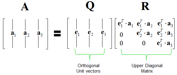
* Collectively we have $\mathbf{X} = \mathbf{Q} \mathbf{R}$.
- $\mathbf{Q} \in \mathbb{R}^{n \times p}$ has orthonormal columns $\mathbf{q}_k$ thus $\mathbf{Q}^T \mathbf{Q} = \mathbf{I}_p$
- Where is $\mathbf{R}$? $\mathbf{R} = \mathbf{Q}^T \mathbf{X}$ has entries $r_{jk} = \langle \mathbf{q}_j, \mathbf{x}_k \rangle$, which are computed during the Gram-Schmidt process. Note $r_{jk} = 0$ for $j > k$, so $\mathbf{R}$ is upper triangular.
* In GS algorithm, $\mathbf{X}$ is over-written by $\mathbf{Q}$ and $\mathbf{R}$ is stored in a separate array.
* The regular Gram-Schmidt is *unstable* (we loose orthogonality due to roundoff errors) when columns of $\mathbf{X}$ are collinear.
* **Modified Gram-Schmidt** (MGS): after each normalization step of $\mathbf{v}_k$, we replace columns $\mathbf{x}_j$, $j>k$, by its residual.
* Why MGS is better than GS? Read
* Computational cost of GS and MGS is $\sum_{k=1}^p 4n(k-1) \approx 2np^2$.
### QR by Householder transform
* Assume $\mathbf{X} = (\mathbf{x}_1, \ldots, \mathbf{x}_p) \in \mathbb{R}^{n \times p}$ has full column rank.
* Gram-Schmidt (GS) algorithm produces the **skinny QR**:
$$
\mathbf{X} = \mathbf{Q} \mathbf{R},
$$
where $\mathbf{Q} \in \mathbb{R}^{n \times p}$ has orthonormal columns and $\mathbf{R} \in \mathbb{R}^{p \times p}$ is an upper triangular matrix.
* **Gram-Schmidt algorithm** orthonormalizes a set of non-zero, *linearly independent* vectors $\mathbf{x}_1,\ldots,\mathbf{x}_p$.
0. Initialize $\mathbf{q}_1 = \mathbf{x}_1 / \|\mathbf{x}_1\|_2$
0. For $k=2, \ldots, p$,
$$
\begin{eqnarray*}
\mathbf{v}_k &=& \mathbf{x}_k - \mathbf{P}_{\mathcal{C} \{\mathbf{q}_1,\ldots,\mathbf{q}_{k-1}\}} \mathbf{x}_k = \mathbf{x}_k - \sum_{j=1}^{k-1} \langle \mathbf{x}_k, \mathbf{q}_j \rangle \cdot \mathbf{q}_j \\
\mathbf{q}_k &=& \mathbf{v}_k / \|\mathbf{v}_k\|_2
\end{eqnarray*}
$$
* Collectively we have $\mathbf{X} = \mathbf{Q} \mathbf{R}$.
- $\mathbf{Q} \in \mathbb{R}^{n \times p}$ has orthonormal columns $\mathbf{q}_k$ thus $\mathbf{Q}^T \mathbf{Q} = \mathbf{I}_p$
- Where is $\mathbf{R}$? $\mathbf{R} = \mathbf{Q}^T \mathbf{X}$ has entries $r_{jk} = \langle \mathbf{q}_j, \mathbf{x}_k \rangle$, which are computed during the Gram-Schmidt process. Note $r_{jk} = 0$ for $j > k$, so $\mathbf{R}$ is upper triangular.
* In GS algorithm, $\mathbf{X}$ is over-written by $\mathbf{Q}$ and $\mathbf{R}$ is stored in a separate array.
* The regular Gram-Schmidt is *unstable* (we loose orthogonality due to roundoff errors) when columns of $\mathbf{X}$ are collinear.
* **Modified Gram-Schmidt** (MGS): after each normalization step of $\mathbf{v}_k$, we replace columns $\mathbf{x}_j$, $j>k$, by its residual.
* Why MGS is better than GS? Read
* Computational cost of GS and MGS is $\sum_{k=1}^p 4n(k-1) \approx 2np^2$.
### QR by Householder transform
 * This is the algorithm implemented in LAPACK. In other words, **this is the algorithm for solving linear regression in R**.
* Assume $\mathbf{X} = (\mathbf{x}_1, \ldots, \mathbf{x}_p) \in \mathbb{R}^{n \times p}$ has full column rank.
* Idea:
$$
\mathbf{H}_{p} \cdots \mathbf{H}_2 \mathbf{H}_1 \mathbf{X} = \begin{pmatrix} \mathbf{R}_1 \\ \mathbf{0} \end{pmatrix},
$$
where $\mathbf{H}_j \in \mathbf{R}^{n \times n}$ are a sequence of Householder transformation matrices.
It yields the **full QR** where $\mathbf{Q} = \mathbf{H}_1 \cdots \mathbf{H}_p \in \mathbb{R}^{n \times n}$. Recall that GS/MGS only produces the **thin QR** decomposition.
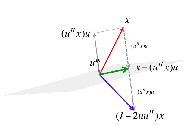
* For arbitrary $\mathbf{v}, \mathbf{w} \in \mathbb{R}^{n}$ with $\|\mathbf{v}\|_2 = \|\mathbf{w}\|_2$, we can construct a **Householder matrix** (or **Householder reflector**)
$$
\mathbf{H} = \mathbf{I}_n - 2 \mathbf{u} \mathbf{u}^T, \quad \mathbf{u} = - \frac{1}{\|\mathbf{v} - \mathbf{w}\|_2} (\mathbf{v} - \mathbf{w}),
$$
that transforms $\mathbf{v}$ to $\mathbf{w}$:
$$
\mathbf{H} \mathbf{v} = \mathbf{w}.
$$
$\mathbf{H}$ is symmetric and orthogonal. Calculation of Householder vector $\mathbf{u}$ costs $4n$ flops for general $\mathbf{u}$ and $\mathbf{w}$.
* This is the algorithm implemented in LAPACK. In other words, **this is the algorithm for solving linear regression in R**.
* Assume $\mathbf{X} = (\mathbf{x}_1, \ldots, \mathbf{x}_p) \in \mathbb{R}^{n \times p}$ has full column rank.
* Idea:
$$
\mathbf{H}_{p} \cdots \mathbf{H}_2 \mathbf{H}_1 \mathbf{X} = \begin{pmatrix} \mathbf{R}_1 \\ \mathbf{0} \end{pmatrix},
$$
where $\mathbf{H}_j \in \mathbf{R}^{n \times n}$ are a sequence of Householder transformation matrices.
It yields the **full QR** where $\mathbf{Q} = \mathbf{H}_1 \cdots \mathbf{H}_p \in \mathbb{R}^{n \times n}$. Recall that GS/MGS only produces the **thin QR** decomposition.
* For arbitrary $\mathbf{v}, \mathbf{w} \in \mathbb{R}^{n}$ with $\|\mathbf{v}\|_2 = \|\mathbf{w}\|_2$, we can construct a **Householder matrix** (or **Householder reflector**)
$$
\mathbf{H} = \mathbf{I}_n - 2 \mathbf{u} \mathbf{u}^T, \quad \mathbf{u} = - \frac{1}{\|\mathbf{v} - \mathbf{w}\|_2} (\mathbf{v} - \mathbf{w}),
$$
that transforms $\mathbf{v}$ to $\mathbf{w}$:
$$
\mathbf{H} \mathbf{v} = \mathbf{w}.
$$
$\mathbf{H}$ is symmetric and orthogonal. Calculation of Householder vector $\mathbf{u}$ costs $4n$ flops for general $\mathbf{u}$ and $\mathbf{w}$.
 * Now choose $\mathbf{H}_1$ to zero the first column of $\mathbf{X}$ below diagonal
$$
\mathbf{H}_1 \mathbf{x}_1 = \begin{pmatrix} \|\mathbf{x}_{1}\|_2 \\ 0 \\ \vdots \\ 0 \end{pmatrix}.
$$
Take $\mathbf{H}_2$ to zero the second column below diagonal; ...
* Now choose $\mathbf{H}_1$ to zero the first column of $\mathbf{X}$ below diagonal
$$
\mathbf{H}_1 \mathbf{x}_1 = \begin{pmatrix} \|\mathbf{x}_{1}\|_2 \\ 0 \\ \vdots \\ 0 \end{pmatrix}.
$$
Take $\mathbf{H}_2$ to zero the second column below diagonal; ...
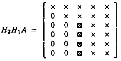 * In general, choose the $j$-th Householder transform $\mathbf{H}_j = \mathbf{I}_n - 2 \mathbf{u}_j \mathbf{u}_j^T$, where
$$
\mathbf{u}_j = \begin{pmatrix} \mathbf{0}_{j-1} \\ {\tilde u}_j \end{pmatrix}, \quad {\tilde u}_j \in \mathbb{R}^{n-j+1},
$$
to zero the $j$-th column below diagonal. $\mathbf{H}_j$ takes the form
$$
\mathbf{H}_j = \begin{pmatrix}
\mathbf{I}_{j-1} & \\
& \mathbf{I}_{n-j+1} - 2 {\tilde u}_j {\tilde u}_j^T
\end{pmatrix} = \begin{pmatrix}
\mathbf{I}_{j-1} & \\
& {\tilde H}_{j}
\end{pmatrix}.
$$
* Applying a Householder transform $\mathbf{H} = \mathbf{I} - 2 \mathbf{u} \mathbf{u}^T$ to a matrix $\mathbf{X} \in \mathbb{R}^{n \times p}$
$$
\mathbf{H} \mathbf{X} = \mathbf{X} - 2 \mathbf{u} (\mathbf{u}^T \mathbf{X})
$$
costs $4np$ flops. **Householder updates never entail explicit formation of the Householder matrices.**
* Note applying ${\tilde H}_j$ to $\mathbf{X}$ only needs $4(n-j+1)(p-j+1)$ flops.
* QR by Householder: $\mathbf{H}_{p} \cdots \mathbf{H}_1 \mathbf{X} = \begin{pmatrix} \mathbf{R}_1 \\ \mathbf{0} \end{pmatrix}$.
* The process is done in place. Upper triangular part of $\mathbf{X}$ is overwritten by $\mathbf{R}_1$ and the essential Householder vectors ($\tilde u_{j1}$ is normalized to 1) are stored in $\mathbf{X}[j:n,j]$.
* At $j$-th stage
0. computing the Householder vector ${\tilde u}_j$ costs $3(n-j+1)$ flops
0. applying the Householder transform ${\tilde H}_j$ to the $\mathbf{X}[j:n, j:p]$ block costs $4(n-j+1)(p-j+1)$ flops
* In total we need
$$
\sum_{j=1}^p [3(n-j+1) + 4(n-j+1)(p-j+1)] \approx 2np^2 - \frac 23 p^3 \quad \text{flops}.
$$
* Where is $\mathbf{Q}$? $\mathbf{Q} = \mathbf{H}_1 \cdots \mathbf{H}_p$. In some applications, it's necessary to form the orthogonal matrix $\mathbf{Q}$.
Accumulating $\mathbf{Q}$ costs another $2np^2 - \frac 23 p^3$ flops.
* When computing $\mathbf{Q}^T \mathbf{v}$ or $\mathbf{Q} \mathbf{v}$ as in some applications (e.g., solve linear equation using QR), no need to form $\mathbf{Q}$. Simply apply Householder transforms successively to the vector $\mathbf{v}$.
* Computational cost of Householder QR for linear regression: $2n p^2 - \frac 23 p^3$ (regression coefficients and $\hat \sigma^2$) or more (fitted values, s.e., ...).
### Householder QR with column pivoting
Consider rank deficient $\mathbf{X}$.
* At the $j$-th stage, swap the column in $\mathbf{X}[j:n,j:p]$ with maximum $\ell_2$ norm to be the pivot column. If the maximum $\ell_2$ norm is 0, it stops, ending with
$$
\mathbf{X} \mathbf{P} = \mathbf{Q} \begin{pmatrix} \mathbf{R}_{11} & \mathbf{R}_{12} \\ \mathbf{0}_{(n-r) \times r} & \mathbf{0}_{(n-r) \times (p-r)} \end{pmatrix},
$$
where $\mathbf{P} \in \mathbb{R}^{p \times p}$ is a permutation matrix and $r$ is the rank of $\mathbf{X}$. QR with column pivoting is rank revealing.
* The overhead of re-computing the column norms can be reduced by the property
$$
\mathbf{Q} \mathbf{z} = \begin{pmatrix} \alpha \\ \omega \end{pmatrix} \Rightarrow \|\omega\|_2^2 = \|\mathbf{z}\|_2^2 - \alpha^2
$$
for any orthogonal matrix $\mathbf{Q}$.
#### LAPACK and Julia implementation
* Julia functions: [qr](https://docs.julialang.org/en/v1/stdlib/LinearAlgebra/#LinearAlgebra.qr), [qr!](https://docs.julialang.org/en/v1/stdlib/LinearAlgebra/#LinearAlgebra.qr!), or call LAPACK wrapper functions [geqrf!](https://docs.julialang.org/en/v1/stdlib/LinearAlgebra/#LinearAlgebra.LAPACK.geqrf!) and [geqp3!](https://docs.julialang.org/en/v1/stdlib/LinearAlgebra/#LinearAlgebra.LAPACK.geqp3!)
```{julia}
using Random, LinearAlgebra
Random.seed!(257) # seed
y = randn(5) # response vector
X = randn(5, 3) # predictor matrix
```
```{julia}
X \ y # least squares solution by QR
```
```{julia}
# same as
qr(X) \ y
```
```{julia}
cholesky(X'X) \ (X'y) # least squares solution by Cholesky
```
```{julia}
# QR factorization with column pivoting
xqr = qr(X, Val(true))
```
```{julia}
xqr \ y # least squares solution
```
```{julia}
# thin Q matrix multiplication (a sequence of Householder transforms)
norm(xqr.Q * xqr.R - X[:, xqr.p]) # recovers X (with columns permuted)
```
### QR by Givens rotation
* Householder transform $\mathbf{H}_j$ introduces batch of zeros into a vector.
* **Givens transform** (aka **Givens rotation**, **Jacobi rotation**, **plane rotation**) selectively zeros one element of a vector.
* Overall QR by Givens rotation is less efficient than the Householder method, but is better suited for matrices with structured patterns of nonzero elements.
* **Givens/Jacobi rotations**:
$$
\mathbf{G}(i,k,\theta) = \begin{pmatrix}
1 & & 0 & & 0 & & 0 \\
\vdots & \ddots & \vdots & & \vdots & & \vdots \\
0 & & c & & s & & 0 \\
\vdots & & \vdots & \ddots & \vdots & & \vdots \\
0 & & - s & & c & & 0 \\
\vdots & & \vdots & & \vdots & \ddots & \vdots \\
0 & & 0 & & 0 & & 1 \end{pmatrix},
$$
where $c = \cos(\theta)$ and $s = \sin(\theta)$. $\mathbf{G}(i,k,\theta)$ is orthogonal.
* Pre-multiplication by $\mathbf{G}(i,k,\theta)^T$ rotates counterclockwise $\theta$ radians in the $(i,k)$ coordinate plane. If $\mathbf{x} \in \mathbb{R}^n$ and $\mathbf{y} = \mathbf{G}(i,k,\theta)^T \mathbf{x}$, then
$$
y_j = \begin{cases}
cx_i - s x_k & j = i \\
sx_i + cx_k & j = k \\
x_j & j \ne i, k
\end{cases}.
$$
Apparently if we choose $\tan(\theta) = -x_k / x_i$, or equivalently,
$$
\begin{eqnarray*}
c = \frac{x_i}{\sqrt{x_i^2 + x_k^2}}, \quad s = \frac{-x_k}{\sqrt{x_i^2 + x_k^2}},
\end{eqnarray*}
$$
then $y_k=0$.
* Pre-applying Givens transform $\mathbf{G}(i,k,\theta)^T \in \mathbb{R}^{n \times n}$ to a matrix $\mathbf{A} \in \mathbb{R}^{n \times m}$ only effects two rows of $\mathbf{
A}$:
$$
\mathbf{A}([i, k], :) \gets \begin{pmatrix} c & s \\ -s & c \end{pmatrix}^T \mathbf{A}([i, k], :),
$$
costing $6m$ flops.
* Post-applying Givens transform $\mathbf{G}(i,k,\theta) \in \mathbb{R}^{m \times m}$ to a matrix $\mathbf{A} \in \mathbb{R}^{n \times m}$ only effects two columns of $\mathbf{A}$:
$$
\mathbf{A}(:, [i,k]) \gets \mathbf{A}(:, [i,k]) \begin{pmatrix} c & s \\ -s & c \end{pmatrix},
$$
costing $6n$ flops.
* QR by Givens: $\mathbf{G}_t^T \cdots \mathbf{G}_1^T \mathbf{X} = \begin{pmatrix} \mathbf{R}_1 \\ \mathbf{0} \end{pmatrix}$.
* In general, choose the $j$-th Householder transform $\mathbf{H}_j = \mathbf{I}_n - 2 \mathbf{u}_j \mathbf{u}_j^T$, where
$$
\mathbf{u}_j = \begin{pmatrix} \mathbf{0}_{j-1} \\ {\tilde u}_j \end{pmatrix}, \quad {\tilde u}_j \in \mathbb{R}^{n-j+1},
$$
to zero the $j$-th column below diagonal. $\mathbf{H}_j$ takes the form
$$
\mathbf{H}_j = \begin{pmatrix}
\mathbf{I}_{j-1} & \\
& \mathbf{I}_{n-j+1} - 2 {\tilde u}_j {\tilde u}_j^T
\end{pmatrix} = \begin{pmatrix}
\mathbf{I}_{j-1} & \\
& {\tilde H}_{j}
\end{pmatrix}.
$$
* Applying a Householder transform $\mathbf{H} = \mathbf{I} - 2 \mathbf{u} \mathbf{u}^T$ to a matrix $\mathbf{X} \in \mathbb{R}^{n \times p}$
$$
\mathbf{H} \mathbf{X} = \mathbf{X} - 2 \mathbf{u} (\mathbf{u}^T \mathbf{X})
$$
costs $4np$ flops. **Householder updates never entail explicit formation of the Householder matrices.**
* Note applying ${\tilde H}_j$ to $\mathbf{X}$ only needs $4(n-j+1)(p-j+1)$ flops.
* QR by Householder: $\mathbf{H}_{p} \cdots \mathbf{H}_1 \mathbf{X} = \begin{pmatrix} \mathbf{R}_1 \\ \mathbf{0} \end{pmatrix}$.
* The process is done in place. Upper triangular part of $\mathbf{X}$ is overwritten by $\mathbf{R}_1$ and the essential Householder vectors ($\tilde u_{j1}$ is normalized to 1) are stored in $\mathbf{X}[j:n,j]$.
* At $j$-th stage
0. computing the Householder vector ${\tilde u}_j$ costs $3(n-j+1)$ flops
0. applying the Householder transform ${\tilde H}_j$ to the $\mathbf{X}[j:n, j:p]$ block costs $4(n-j+1)(p-j+1)$ flops
* In total we need
$$
\sum_{j=1}^p [3(n-j+1) + 4(n-j+1)(p-j+1)] \approx 2np^2 - \frac 23 p^3 \quad \text{flops}.
$$
* Where is $\mathbf{Q}$? $\mathbf{Q} = \mathbf{H}_1 \cdots \mathbf{H}_p$. In some applications, it's necessary to form the orthogonal matrix $\mathbf{Q}$.
Accumulating $\mathbf{Q}$ costs another $2np^2 - \frac 23 p^3$ flops.
* When computing $\mathbf{Q}^T \mathbf{v}$ or $\mathbf{Q} \mathbf{v}$ as in some applications (e.g., solve linear equation using QR), no need to form $\mathbf{Q}$. Simply apply Householder transforms successively to the vector $\mathbf{v}$.
* Computational cost of Householder QR for linear regression: $2n p^2 - \frac 23 p^3$ (regression coefficients and $\hat \sigma^2$) or more (fitted values, s.e., ...).
### Householder QR with column pivoting
Consider rank deficient $\mathbf{X}$.
* At the $j$-th stage, swap the column in $\mathbf{X}[j:n,j:p]$ with maximum $\ell_2$ norm to be the pivot column. If the maximum $\ell_2$ norm is 0, it stops, ending with
$$
\mathbf{X} \mathbf{P} = \mathbf{Q} \begin{pmatrix} \mathbf{R}_{11} & \mathbf{R}_{12} \\ \mathbf{0}_{(n-r) \times r} & \mathbf{0}_{(n-r) \times (p-r)} \end{pmatrix},
$$
where $\mathbf{P} \in \mathbb{R}^{p \times p}$ is a permutation matrix and $r$ is the rank of $\mathbf{X}$. QR with column pivoting is rank revealing.
* The overhead of re-computing the column norms can be reduced by the property
$$
\mathbf{Q} \mathbf{z} = \begin{pmatrix} \alpha \\ \omega \end{pmatrix} \Rightarrow \|\omega\|_2^2 = \|\mathbf{z}\|_2^2 - \alpha^2
$$
for any orthogonal matrix $\mathbf{Q}$.
#### LAPACK and Julia implementation
* Julia functions: [qr](https://docs.julialang.org/en/v1/stdlib/LinearAlgebra/#LinearAlgebra.qr), [qr!](https://docs.julialang.org/en/v1/stdlib/LinearAlgebra/#LinearAlgebra.qr!), or call LAPACK wrapper functions [geqrf!](https://docs.julialang.org/en/v1/stdlib/LinearAlgebra/#LinearAlgebra.LAPACK.geqrf!) and [geqp3!](https://docs.julialang.org/en/v1/stdlib/LinearAlgebra/#LinearAlgebra.LAPACK.geqp3!)
```{julia}
using Random, LinearAlgebra
Random.seed!(257) # seed
y = randn(5) # response vector
X = randn(5, 3) # predictor matrix
```
```{julia}
X \ y # least squares solution by QR
```
```{julia}
# same as
qr(X) \ y
```
```{julia}
cholesky(X'X) \ (X'y) # least squares solution by Cholesky
```
```{julia}
# QR factorization with column pivoting
xqr = qr(X, Val(true))
```
```{julia}
xqr \ y # least squares solution
```
```{julia}
# thin Q matrix multiplication (a sequence of Householder transforms)
norm(xqr.Q * xqr.R - X[:, xqr.p]) # recovers X (with columns permuted)
```
### QR by Givens rotation
* Householder transform $\mathbf{H}_j$ introduces batch of zeros into a vector.
* **Givens transform** (aka **Givens rotation**, **Jacobi rotation**, **plane rotation**) selectively zeros one element of a vector.
* Overall QR by Givens rotation is less efficient than the Householder method, but is better suited for matrices with structured patterns of nonzero elements.
* **Givens/Jacobi rotations**:
$$
\mathbf{G}(i,k,\theta) = \begin{pmatrix}
1 & & 0 & & 0 & & 0 \\
\vdots & \ddots & \vdots & & \vdots & & \vdots \\
0 & & c & & s & & 0 \\
\vdots & & \vdots & \ddots & \vdots & & \vdots \\
0 & & - s & & c & & 0 \\
\vdots & & \vdots & & \vdots & \ddots & \vdots \\
0 & & 0 & & 0 & & 1 \end{pmatrix},
$$
where $c = \cos(\theta)$ and $s = \sin(\theta)$. $\mathbf{G}(i,k,\theta)$ is orthogonal.
* Pre-multiplication by $\mathbf{G}(i,k,\theta)^T$ rotates counterclockwise $\theta$ radians in the $(i,k)$ coordinate plane. If $\mathbf{x} \in \mathbb{R}^n$ and $\mathbf{y} = \mathbf{G}(i,k,\theta)^T \mathbf{x}$, then
$$
y_j = \begin{cases}
cx_i - s x_k & j = i \\
sx_i + cx_k & j = k \\
x_j & j \ne i, k
\end{cases}.
$$
Apparently if we choose $\tan(\theta) = -x_k / x_i$, or equivalently,
$$
\begin{eqnarray*}
c = \frac{x_i}{\sqrt{x_i^2 + x_k^2}}, \quad s = \frac{-x_k}{\sqrt{x_i^2 + x_k^2}},
\end{eqnarray*}
$$
then $y_k=0$.
* Pre-applying Givens transform $\mathbf{G}(i,k,\theta)^T \in \mathbb{R}^{n \times n}$ to a matrix $\mathbf{A} \in \mathbb{R}^{n \times m}$ only effects two rows of $\mathbf{
A}$:
$$
\mathbf{A}([i, k], :) \gets \begin{pmatrix} c & s \\ -s & c \end{pmatrix}^T \mathbf{A}([i, k], :),
$$
costing $6m$ flops.
* Post-applying Givens transform $\mathbf{G}(i,k,\theta) \in \mathbb{R}^{m \times m}$ to a matrix $\mathbf{A} \in \mathbb{R}^{n \times m}$ only effects two columns of $\mathbf{A}$:
$$
\mathbf{A}(:, [i,k]) \gets \mathbf{A}(:, [i,k]) \begin{pmatrix} c & s \\ -s & c \end{pmatrix},
$$
costing $6n$ flops.
* QR by Givens: $\mathbf{G}_t^T \cdots \mathbf{G}_1^T \mathbf{X} = \begin{pmatrix} \mathbf{R}_1 \\ \mathbf{0} \end{pmatrix}$.
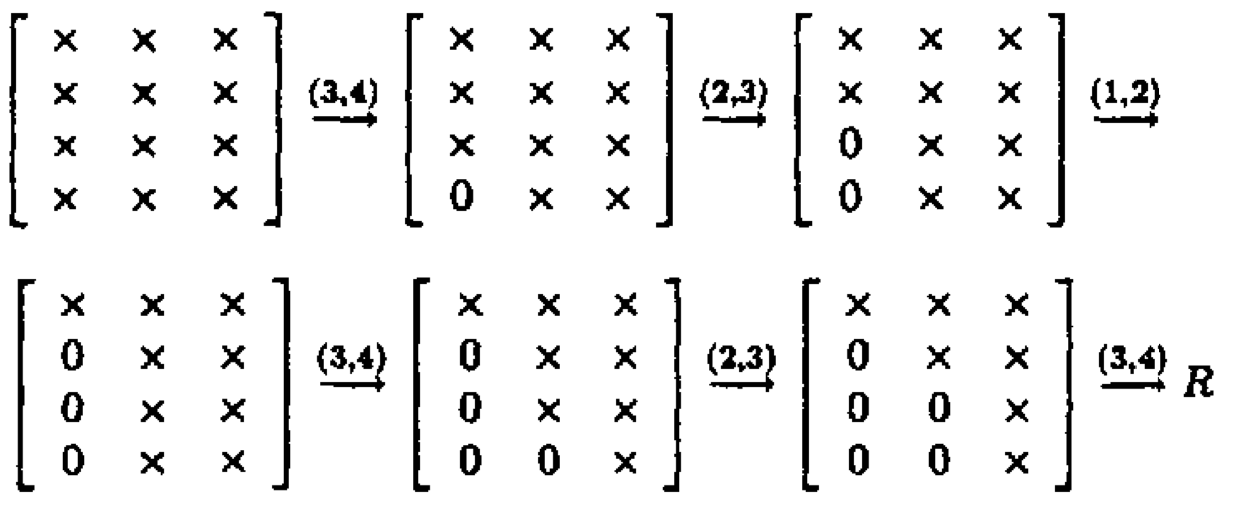 * Zeros in $\mathbf{X}$ can also be introduced row-by-row.
* If $\mathbf{X} \in \mathbb{R}^{n \times p}$, the total cost is $3np^2 - p^3$ flops and $O(np)$ square roots.
* Note each Givens transform can be summarized by a single number, which is stored in the zeroed entry of $\mathbf{X}$.
* *Fast Givens transform* avoids taking square roots.
## Applications
### Linear regression
* QR decomposition of $\mathbf{X}$: $2np^2 - \frac 23 p^3$ flops.
* Solve $\mathbf{R}^T \mathbf{R} \beta = \mathbf{R}^T \mathbf{Q} \mathbf{y}$ for $\beta$.
* If need standard errors, compute inverse of $\mathbf{R}^T \mathbf{R}$.
## Further reading
* Section 7.8 of [Numerical Analysis for Statisticians](http://ucla.worldcat.org/title/numerical-analysis-for-statisticians/oclc/793808354&referer=brief_results) of Kenneth Lange (2010).
* Section II.5.3 of [Computational Statistics](http://ucla.worldcat.org/title/computational-statistics/oclc/437345409&referer=brief_results) by James Gentle (2010).
* Chapter 5 of [Matrix Computation](https://search.library.ucla.edu/permalink/01UCS_LAL/17p22dp/alma9971220883606533) by Gene Golub and Charles Van Loan (2013).
* Zeros in $\mathbf{X}$ can also be introduced row-by-row.
* If $\mathbf{X} \in \mathbb{R}^{n \times p}$, the total cost is $3np^2 - p^3$ flops and $O(np)$ square roots.
* Note each Givens transform can be summarized by a single number, which is stored in the zeroed entry of $\mathbf{X}$.
* *Fast Givens transform* avoids taking square roots.
## Applications
### Linear regression
* QR decomposition of $\mathbf{X}$: $2np^2 - \frac 23 p^3$ flops.
* Solve $\mathbf{R}^T \mathbf{R} \beta = \mathbf{R}^T \mathbf{Q} \mathbf{y}$ for $\beta$.
* If need standard errors, compute inverse of $\mathbf{R}^T \mathbf{R}$.
## Further reading
* Section 7.8 of [Numerical Analysis for Statisticians](http://ucla.worldcat.org/title/numerical-analysis-for-statisticians/oclc/793808354&referer=brief_results) of Kenneth Lange (2010).
* Section II.5.3 of [Computational Statistics](http://ucla.worldcat.org/title/computational-statistics/oclc/437345409&referer=brief_results) by James Gentle (2010).
* Chapter 5 of [Matrix Computation](https://search.library.ucla.edu/permalink/01UCS_LAL/17p22dp/alma9971220883606533) by Gene Golub and Charles Van Loan (2013).