---
title: Conjugate Gradient and Krylov Subspace Methods
subtitle: Biostat/Biomath M257
author: Dr. Hua Zhou @ UCLA
date: today
format:
html:
theme: cosmo
embed-resources: true
number-sections: true
toc: true
toc-depth: 4
toc-location: left
code-fold: false
jupyter:
jupytext:
formats: 'ipynb,qmd'
text_representation:
extension: .qmd
format_name: quarto
format_version: '1.0'
jupytext_version: 1.14.5
kernelspec:
display_name: Julia (8 threads) 1.8.5
language: julia
name: julia-_8-threads_-1.8
---
System information (for reproducibility):
```{julia}
versioninfo()
```
Load packages:
```{julia}
using Pkg
Pkg.activate(pwd())
Pkg.instantiate()
Pkg.status()
```
## Introduction
* Conjugate gradient is the top-notch iterative method for solving large, **structured** linear systems $\mathbf{A} \mathbf{x} = \mathbf{b}$, where $\mathbf{A}$ is pd.
Earlier we talked about Jacobi, Gauss-Seidel, and successive over-relaxation (SOR) as the classical iterative solvers. They are rarely used in practice due to slow convergence.
[Kershaw's results](http://www.sciencedirect.com/science/article/pii/0021999178900980?via%3Dihub) for a fusion problem.
| Method | Number of Iterations |
|----------------------------------------|----------------------|
| Gauss Seidel | 208,000 |
| Block SOR methods | 765 |
| Incomplete Cholesky **conjugate gradient** | 25 |
* History: Hestenes (**UCLA** professor!) and Stiefel proposed conjugate gradient method in 1950s.
Hestenes and Stiefel (1952), [Methods of conjugate gradients for solving linear systems](http://nvlpubs.nist.gov/nistpubs/jres/049/jresv49n6p409_A1b.pdf), _Jounral of Research of the National Bureau of Standards_.
* Solve linear equation $\mathbf{A} \mathbf{x} = \mathbf{b}$, where $\mathbf{A} \in \mathbb{R}^{n \times n}$ is **pd**, is equivalent to
$$
\begin{eqnarray*}
\text{minimize} \,\, f(\mathbf{x}) = \frac 12 \mathbf{x}^T \mathbf{A} \mathbf{x} - \mathbf{b}^T \mathbf{x}.
\end{eqnarray*}
$$
Denote $\nabla f(\mathbf{x}) = \mathbf{A} \mathbf{x} - \mathbf{b} =: r(\mathbf{x})$.
## Conjugate gradient (CG) method
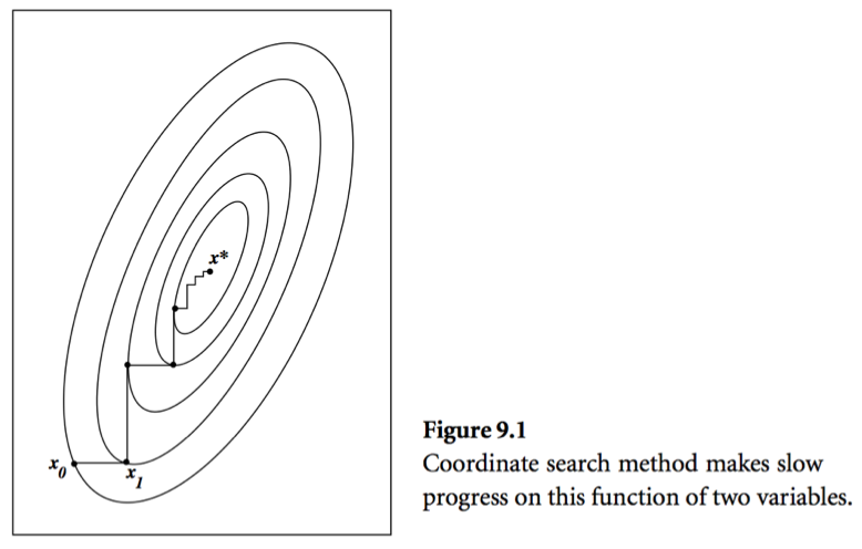
* Consider a simple idea: coordinate descent, that is to update components $x_j$ alternatingly. Same as the Gauss-Seidel iteration. Usually it takes too many iterations.
 * A set of vectors $\{\mathbf{p}^{(0)},\ldots,\mathbf{p}^{(l)}\}$ is said to be **conjugate with respect to $\mathbf{A}$** if
$$
\begin{eqnarray*}
\mathbf{p}_i^T \mathbf{A} \mathbf{p}_j = 0, \quad \text{for all } i \ne j.
\end{eqnarray*}
$$
For example, eigen-vectors of $\mathbf{A}$ are conjugate to each other. Why?
* **Conjugate direction** method: Given a set of conjugate vectors $\{\mathbf{p}^{(0)},\ldots,\mathbf{p}^{(l)}\}$, at iteration $t$, we search along the conjugate direction $\mathbf{p}^{(t)}$
$$
\begin{eqnarray*}
\mathbf{x}^{(t+1)} = \mathbf{x}^{(t)} + \alpha^{(t)} \mathbf{p}^{(t)},
\end{eqnarray*}
$$
where
$$
\begin{eqnarray*}
\alpha^{(t)} = - \frac{\mathbf{r}^{(t)T} \mathbf{p}^{(t)}}{\mathbf{p}^{(t)T} \mathbf{A} \mathbf{p}^{(t)}}
\end{eqnarray*}
$$
is the optimal step length.
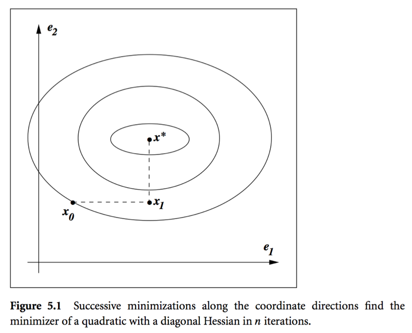
* Theorem: In conjugate direction method, $\mathbf{x}^{(t)}$ converges to the solution in **at most** $n$ steps.
Intuition: Look at graph.
* A set of vectors $\{\mathbf{p}^{(0)},\ldots,\mathbf{p}^{(l)}\}$ is said to be **conjugate with respect to $\mathbf{A}$** if
$$
\begin{eqnarray*}
\mathbf{p}_i^T \mathbf{A} \mathbf{p}_j = 0, \quad \text{for all } i \ne j.
\end{eqnarray*}
$$
For example, eigen-vectors of $\mathbf{A}$ are conjugate to each other. Why?
* **Conjugate direction** method: Given a set of conjugate vectors $\{\mathbf{p}^{(0)},\ldots,\mathbf{p}^{(l)}\}$, at iteration $t$, we search along the conjugate direction $\mathbf{p}^{(t)}$
$$
\begin{eqnarray*}
\mathbf{x}^{(t+1)} = \mathbf{x}^{(t)} + \alpha^{(t)} \mathbf{p}^{(t)},
\end{eqnarray*}
$$
where
$$
\begin{eqnarray*}
\alpha^{(t)} = - \frac{\mathbf{r}^{(t)T} \mathbf{p}^{(t)}}{\mathbf{p}^{(t)T} \mathbf{A} \mathbf{p}^{(t)}}
\end{eqnarray*}
$$
is the optimal step length.
* Theorem: In conjugate direction method, $\mathbf{x}^{(t)}$ converges to the solution in **at most** $n$ steps.
Intuition: Look at graph.
 * **Conjugate gradient** method. Idea: generate $\mathbf{p}^{(t)}$ using only $\mathbf{p}^{(t-1)}$
$$
\begin{eqnarray*}
\mathbf{p}^{(t)} = - \mathbf{r}^{(t)} + \beta^{(t)} \mathbf{p}^{(t-1)},
\end{eqnarray*}
$$
where $\beta^{(t)}$ is determined by the conjugacy condition $\mathbf{p}^{(t-1)T} \mathbf{A} \mathbf{p}^{(t)} = 0$
$$
\begin{eqnarray*}
\beta^{(t)} = \frac{\mathbf{r}^{(t)T} \mathbf{A} \mathbf{p}^{(t-1)}}{\mathbf{p}^{(t-1)T} \mathbf{A} \mathbf{p}^{(t-1)}}.
\end{eqnarray*}
$$
* **CG algorithm (preliminary version)**:
0. Given $\mathbf{x}^{(0)}$
0. Initialize: $\mathbf{r}^{(0)} \gets \mathbf{A} \mathbf{x}^{(0)} - \mathbf{b}$, $\mathbf{p}^{(0)} \gets - \mathbf{r}^{(0)}$, $t=0$
0. While $\mathbf{r}^{(t)} \ne \mathbf{0}$
1. $\alpha^{(t)} \gets - \frac{\mathbf{r}^{(t)T} \mathbf{p}^{(t)}}{\mathbf{p}^{(t)T} \mathbf{A} \mathbf{p}^{(t)}}$
2. $\mathbf{x}^{(t+1)} \gets \mathbf{x}^{(t)} + \alpha^{(t)} \mathbf{p}^{(t)}$
3. $\mathbf{r}^{(t+1)} \gets \mathbf{A} \mathbf{x}^{(t+1)} - \mathbf{b}$
4. $\beta^{(t+1)} \gets \frac{\mathbf{r}^{(t+1)T} \mathbf{A} \mathbf{p}^{(t)}}{\mathbf{p}^{(t)T} \mathbf{A} \mathbf{p}^{(t)}}$
5. $\mathbf{p}^{(t+1)} \gets - \mathbf{r}^{(t+1)} + \beta^{(t+1)} \mathbf{p}^{(t)}$
6. $t \gets t+1$
Remark: The initial conjugate direction $\mathbf{p}^{(0)} \gets - \mathbf{r}^{(0)}$ is crucial.
* Theorem: With CG algorithm
0. $\mathbf{r}^{(t)}$ are mutually orthogonal.
0. $\{\mathbf{r}^{(0)},\ldots,\mathbf{r}^{(t)}\}$ is contained in the **Krylov subspace** of degree $t$ for $\mathbf{r}^{(0)}$, denoted by
$$
\begin{eqnarray*}
{\cal K}(\mathbf{r}^{(0)}; t) = \text{span} \{\mathbf{r}^{(0)},\mathbf{A} \mathbf{r}^{(0)}, \mathbf{A}^2 \mathbf{r}^{(0)}, \ldots, \mathbf{A}^{t} \mathbf{r}^{(0)}\}.
\end{eqnarray*}
$$
0. $\{\mathbf{p}^{(0)},\ldots,\mathbf{p}^{(t)}\}$ is contained in ${\cal K}(\mathbf{r}^{(0)}; t)$.
0. $\mathbf{p}^{(0)}, \ldots, \mathbf{p}^{(t)}$ are conjugate with respect to $\mathbf{A}$.
The iterates $\mathbf{x}^{(t)}$ converge to the solution in at most $n$ steps.
* **CG algorithm (economical version)**: saves one matrix-vector multiplication.
0. Given $\mathbf{x}^{(0)}$
0. Initialize: $\mathbf{r}^{(0)} \gets \mathbf{A} \mathbf{x}^{(0)} - \mathbf{b}$, $\mathbf{p}^{(0)} \gets - \mathbf{r}^{(0)}$, $t=0$
0. While $\mathbf{r}^{(t)} \ne \mathbf{0}$
1. $\alpha^{(t)} \gets \frac{\mathbf{r}^{(t)T} \mathbf{r}^{(t)}}{\mathbf{p}^{(t)T} \mathbf{A} \mathbf{p}^{(t)}}$
2. $\mathbf{x}^{(t+1)} \gets \mathbf{x}^{(t)} + \alpha^{(t)} \mathbf{p}^{(t)}$
3. $\mathbf{r}^{(t+1)} \gets \mathbf{r}^{(t)} + \alpha^{(t)} \mathbf{A} \mathbf{p}^{(t)}$
4. $\beta^{(t+1)} \gets \frac{\mathbf{r}^{(t+1)T} \mathbf{r}^{(t+1)}}{\mathbf{r}^{(t)T} \mathbf{r}^{(t)}}$
5. $\mathbf{p}^{(t+1)} \gets - \mathbf{r}^{(t+1)} + \beta^{(t+1)} \mathbf{p}^{(t)}$
6. $t \gets t+1$
* Computation cost per iteration is **one** matrix vector multiplication: $\mathbf{A} \mathbf{p}^{(t)}$.
Consider PageRank problem, $\mathbf{A}$ has dimension $n \approx 10^{10}$ but is highly structured (sparse + low rank). Each matrix vector multiplication takes $O(n)$.
* Theorem: If $\mathbf{A}$ has $r$ distinct eigenvalues, $\mathbf{x}^{(t)}$ converges to solution $\mathbf{x}^*$ in at most $r$ steps.
## Pre-conditioned conjugate gradient (PCG)
* Summary of conjugate gradient method for solving $\mathbf{A} \mathbf{x} = \mathbf{b}$ or equivalently minimizing $\frac 12 \mathbf{x}^T \mathbf{A} \mathbf{x} - \mathbf{b}^T \mathbf{x}$:
* Each iteration needs one matrix vector multiplication: $\mathbf{A} \mathbf{p}^{(t+1)}$. For structured $\mathbf{A}$, often $O(n)$ cost per iteration.
* Guaranteed to converge in $n$ steps.
* Two important bounds for conjugate gradient algorithm:
Let $\lambda_1 \le \cdots \le \lambda_n$ be the ordered eigenvalues of a pd $\mathbf{A}$.
$$
\begin{eqnarray*}
\|\mathbf{x}^{(t+1)} - \mathbf{x}^*\|_{\mathbf{A}}^2 &\le& \left( \frac{\lambda_{n-t} - \lambda_1}{\lambda_{n-t} + \lambda_1} \right)^2 \|\mathbf{x}^{(0)} - \mathbf{x}^*\|_{\mathbf{A}}^2 \\
\|\mathbf{x}^{(t+1)} - \mathbf{x}^*\|_{\mathbf{A}}^2 &\le& 2 \left( \frac{\sqrt{\kappa(\mathbf{A})}-1}{\sqrt{\kappa(\mathbf{A})}+1} \right)^{t} \|\mathbf{x}^{(0)} - \mathbf{x}^*\|_{\mathbf{A}}^2,
\end{eqnarray*}
$$
where $\kappa(\mathbf{A}) = \lambda_n/\lambda_1$ is the condition number of $\mathbf{A}$.
* **Conjugate gradient** method. Idea: generate $\mathbf{p}^{(t)}$ using only $\mathbf{p}^{(t-1)}$
$$
\begin{eqnarray*}
\mathbf{p}^{(t)} = - \mathbf{r}^{(t)} + \beta^{(t)} \mathbf{p}^{(t-1)},
\end{eqnarray*}
$$
where $\beta^{(t)}$ is determined by the conjugacy condition $\mathbf{p}^{(t-1)T} \mathbf{A} \mathbf{p}^{(t)} = 0$
$$
\begin{eqnarray*}
\beta^{(t)} = \frac{\mathbf{r}^{(t)T} \mathbf{A} \mathbf{p}^{(t-1)}}{\mathbf{p}^{(t-1)T} \mathbf{A} \mathbf{p}^{(t-1)}}.
\end{eqnarray*}
$$
* **CG algorithm (preliminary version)**:
0. Given $\mathbf{x}^{(0)}$
0. Initialize: $\mathbf{r}^{(0)} \gets \mathbf{A} \mathbf{x}^{(0)} - \mathbf{b}$, $\mathbf{p}^{(0)} \gets - \mathbf{r}^{(0)}$, $t=0$
0. While $\mathbf{r}^{(t)} \ne \mathbf{0}$
1. $\alpha^{(t)} \gets - \frac{\mathbf{r}^{(t)T} \mathbf{p}^{(t)}}{\mathbf{p}^{(t)T} \mathbf{A} \mathbf{p}^{(t)}}$
2. $\mathbf{x}^{(t+1)} \gets \mathbf{x}^{(t)} + \alpha^{(t)} \mathbf{p}^{(t)}$
3. $\mathbf{r}^{(t+1)} \gets \mathbf{A} \mathbf{x}^{(t+1)} - \mathbf{b}$
4. $\beta^{(t+1)} \gets \frac{\mathbf{r}^{(t+1)T} \mathbf{A} \mathbf{p}^{(t)}}{\mathbf{p}^{(t)T} \mathbf{A} \mathbf{p}^{(t)}}$
5. $\mathbf{p}^{(t+1)} \gets - \mathbf{r}^{(t+1)} + \beta^{(t+1)} \mathbf{p}^{(t)}$
6. $t \gets t+1$
Remark: The initial conjugate direction $\mathbf{p}^{(0)} \gets - \mathbf{r}^{(0)}$ is crucial.
* Theorem: With CG algorithm
0. $\mathbf{r}^{(t)}$ are mutually orthogonal.
0. $\{\mathbf{r}^{(0)},\ldots,\mathbf{r}^{(t)}\}$ is contained in the **Krylov subspace** of degree $t$ for $\mathbf{r}^{(0)}$, denoted by
$$
\begin{eqnarray*}
{\cal K}(\mathbf{r}^{(0)}; t) = \text{span} \{\mathbf{r}^{(0)},\mathbf{A} \mathbf{r}^{(0)}, \mathbf{A}^2 \mathbf{r}^{(0)}, \ldots, \mathbf{A}^{t} \mathbf{r}^{(0)}\}.
\end{eqnarray*}
$$
0. $\{\mathbf{p}^{(0)},\ldots,\mathbf{p}^{(t)}\}$ is contained in ${\cal K}(\mathbf{r}^{(0)}; t)$.
0. $\mathbf{p}^{(0)}, \ldots, \mathbf{p}^{(t)}$ are conjugate with respect to $\mathbf{A}$.
The iterates $\mathbf{x}^{(t)}$ converge to the solution in at most $n$ steps.
* **CG algorithm (economical version)**: saves one matrix-vector multiplication.
0. Given $\mathbf{x}^{(0)}$
0. Initialize: $\mathbf{r}^{(0)} \gets \mathbf{A} \mathbf{x}^{(0)} - \mathbf{b}$, $\mathbf{p}^{(0)} \gets - \mathbf{r}^{(0)}$, $t=0$
0. While $\mathbf{r}^{(t)} \ne \mathbf{0}$
1. $\alpha^{(t)} \gets \frac{\mathbf{r}^{(t)T} \mathbf{r}^{(t)}}{\mathbf{p}^{(t)T} \mathbf{A} \mathbf{p}^{(t)}}$
2. $\mathbf{x}^{(t+1)} \gets \mathbf{x}^{(t)} + \alpha^{(t)} \mathbf{p}^{(t)}$
3. $\mathbf{r}^{(t+1)} \gets \mathbf{r}^{(t)} + \alpha^{(t)} \mathbf{A} \mathbf{p}^{(t)}$
4. $\beta^{(t+1)} \gets \frac{\mathbf{r}^{(t+1)T} \mathbf{r}^{(t+1)}}{\mathbf{r}^{(t)T} \mathbf{r}^{(t)}}$
5. $\mathbf{p}^{(t+1)} \gets - \mathbf{r}^{(t+1)} + \beta^{(t+1)} \mathbf{p}^{(t)}$
6. $t \gets t+1$
* Computation cost per iteration is **one** matrix vector multiplication: $\mathbf{A} \mathbf{p}^{(t)}$.
Consider PageRank problem, $\mathbf{A}$ has dimension $n \approx 10^{10}$ but is highly structured (sparse + low rank). Each matrix vector multiplication takes $O(n)$.
* Theorem: If $\mathbf{A}$ has $r$ distinct eigenvalues, $\mathbf{x}^{(t)}$ converges to solution $\mathbf{x}^*$ in at most $r$ steps.
## Pre-conditioned conjugate gradient (PCG)
* Summary of conjugate gradient method for solving $\mathbf{A} \mathbf{x} = \mathbf{b}$ or equivalently minimizing $\frac 12 \mathbf{x}^T \mathbf{A} \mathbf{x} - \mathbf{b}^T \mathbf{x}$:
* Each iteration needs one matrix vector multiplication: $\mathbf{A} \mathbf{p}^{(t+1)}$. For structured $\mathbf{A}$, often $O(n)$ cost per iteration.
* Guaranteed to converge in $n$ steps.
* Two important bounds for conjugate gradient algorithm:
Let $\lambda_1 \le \cdots \le \lambda_n$ be the ordered eigenvalues of a pd $\mathbf{A}$.
$$
\begin{eqnarray*}
\|\mathbf{x}^{(t+1)} - \mathbf{x}^*\|_{\mathbf{A}}^2 &\le& \left( \frac{\lambda_{n-t} - \lambda_1}{\lambda_{n-t} + \lambda_1} \right)^2 \|\mathbf{x}^{(0)} - \mathbf{x}^*\|_{\mathbf{A}}^2 \\
\|\mathbf{x}^{(t+1)} - \mathbf{x}^*\|_{\mathbf{A}}^2 &\le& 2 \left( \frac{\sqrt{\kappa(\mathbf{A})}-1}{\sqrt{\kappa(\mathbf{A})}+1} \right)^{t} \|\mathbf{x}^{(0)} - \mathbf{x}^*\|_{\mathbf{A}}^2,
\end{eqnarray*}
$$
where $\kappa(\mathbf{A}) = \lambda_n/\lambda_1$ is the condition number of $\mathbf{A}$.
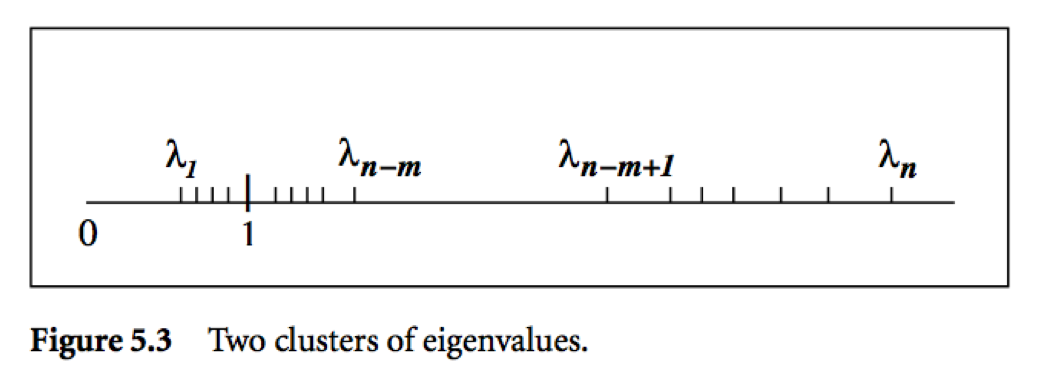
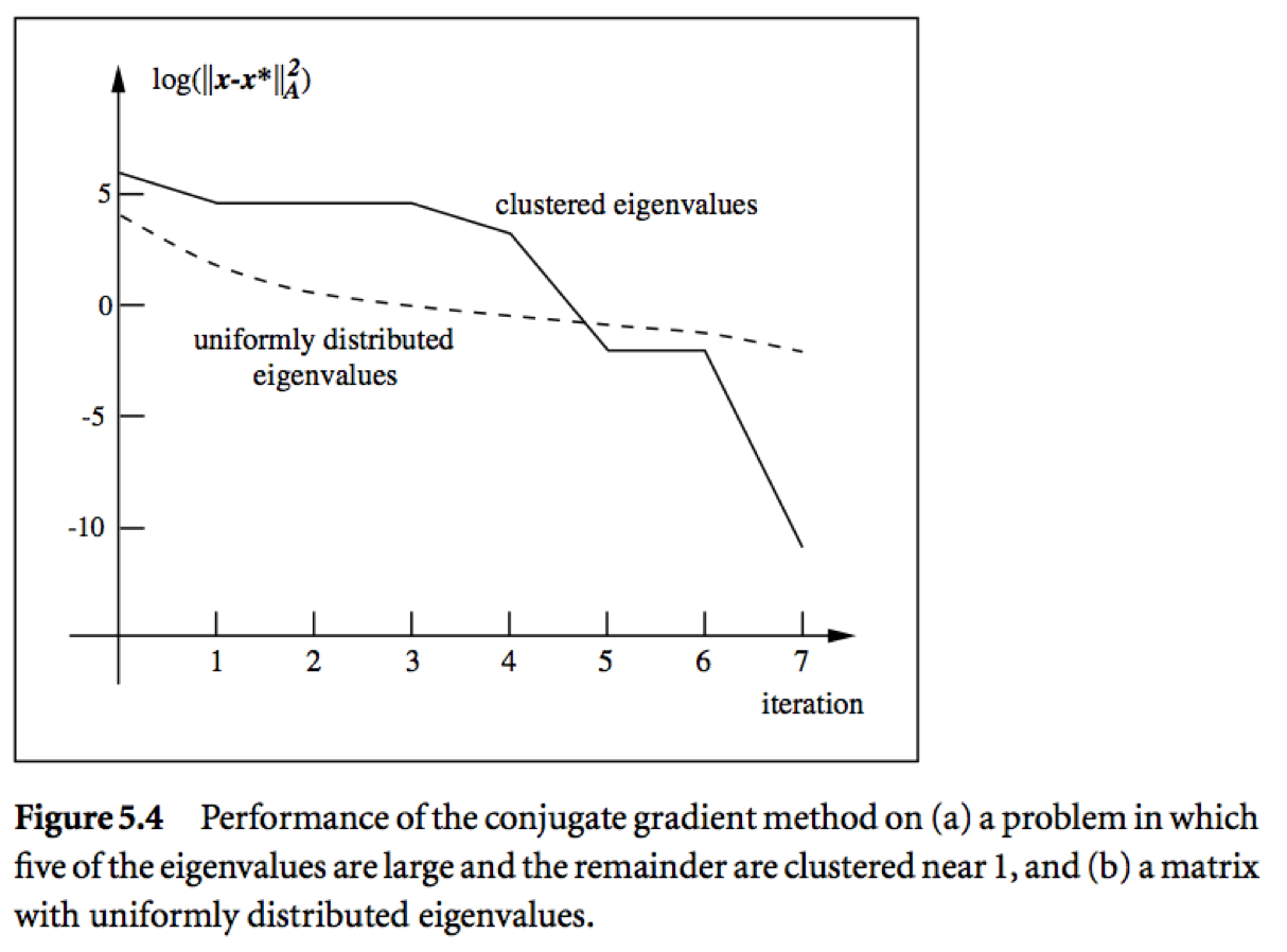 * Messages:
* Roughly speaking, if the eigenvalues of $\mathbf{A}$ occur in $r$ distinct clusters, the CG iterates will _approximately_ solve the problem after $O(r)$ steps.
* $\mathbf{A}$ with a small condition number ($\lambda_1 \approx \lambda_n$) converges fast.
* **Pre-conditioning**: Change of variables $\widehat{\mathbf{x}} = \mathbf{C} \mathbf{x}$ via a nonsingular $\mathbf{C}$ and solve
$$
(\mathbf{C}^{-T} \mathbf{A} \mathbf{C}^{-1}) \widehat{\mathbf{x}} = \mathbf{C}^{-T} \mathbf{b}.
$$
Choose $\mathbf{C}$ such that
* $\mathbf{C}^{-T} \mathbf{A} \mathbf{C}^{-1}$ has small condition number, or
* $\mathbf{C}^{-T} \mathbf{A} \mathbf{C}^{-1}$ has clustered eigenvalues
* Inexpensive solution of $\mathbf{C}^T \mathbf{C} \mathbf{y} = \mathbf{r}$
* Preconditioned CG does not make use of $\mathbf{C}$ explicitly, but rather the matrix $\mathbf{M} = \mathbf{C}^T \mathbf{C}$.
* **Preconditioned CG (PCG)** algorithm:
0. Given $\mathbf{x}^{(0)}$, pre-conditioner $\mathbf{M}$
0. $\mathbf{r}^{(0)} \gets \mathbf{A} \mathbf{x}^{(0)} - \mathbf{b}$
0. solve $\mathbf{M} \mathbf{y}^{(0)} = \mathbf{r}^{(0)}$ for $\mathbf{y}^{(0)}$
0. $\mathbf{p}^{(0)} \gets - \mathbf{r}^{(0)}$, $t=0$
0. While $\mathbf{r}^{(t)} \ne \mathbf{0}$
1. $\alpha^{(t)} \gets \frac{\mathbf{r}^{(t)T} \mathbf{y}^{(t)}}{\mathbf{p}^{(t)T} \mathbf{A} \mathbf{p}^{(t)}}$
2. $\mathbf{x}^{(t+1)} \gets \mathbf{x}^{(t)} + \alpha^{(t)} \mathbf{p}^{(t)}$
3. $\mathbf{r}^{(t+1)} \gets \mathbf{r}^{(t)} + \alpha^{(t)} \mathbf{A} \mathbf{p}^{(t)}$
4. Solve $\mathbf{M} \mathbf{y}^{(t+1)} \gets \mathbf{r}^{(t+1)}$ for $\mathbf{y}^{(t+1)}$
5. $\beta^{(t+1)} \gets \frac{\mathbf{r}^{(t+1)T} \mathbf{y}^{(t+1)}}{\mathbf{r}^{(t)T} \mathbf{r}^{(t)}}$
6. $\mathbf{p}^{(t+1)} \gets - \mathbf{y}^{(t+1)} + \beta^{(t+1)} \mathbf{p}^{(t)}$
7. $t \gets t+1$
Remark: Only extra cost in the pre-conditioned CG algorithm is the need to solve the linear system $\mathbf{M} \mathbf{y} = \mathbf{r}$.
* Pre-conditioning is more like an art than science. Some choices include
* Incomplete Cholesky. $\mathbf{A} \approx \tilde{\mathbf{L}} \tilde{\mathbf{L}}^T$, where $\tilde{\mathbf{L}}$ is a sparse approximate Cholesky factor. Then $\tilde{\mathbf{L}}^{-1} \mathbf{A} \tilde{\mathbf{L}}^{-T} \approx \mathbf{I}$ (perfectly conditioned) and $\mathbf{M} \mathbf{y} = \tilde{\mathbf{L}} \tilde {\mathbf{L}}^T \mathbf{y} = \mathbf{r}$ is easy to solve.
* Banded pre-conditioners.
* Choose $\mathbf{M}$ as a coarsened version of $\mathbf{A}$.
* Subject knowledge. Knowledge about the structure and origin of a problem is often the key to devising efficient pre-conditioner. For example, see recent work of Stein, Chen, Anitescu (2012) for pre-conditioning large covariance matrices. http://epubs.siam.org/doi/abs/10.1137/110834469
### Example of PCG
[Preconditioners.jl](https://github.com/mohamed82008/Preconditioners.jl) wraps a bunch of preconditioners.
We use the Wathen matrix (sparse and positive definite) as a test matrix.
```{julia}
using BenchmarkTools, MatrixDepot, IterativeSolvers, LinearAlgebra, SparseArrays
# Wathen matrix of dimension 30401 x 30401
A = matrixdepot("wathen", 100)
```
```{julia}
using UnicodePlots
spy(A)
```
```{julia}
# sparsity level
count(!iszero, A) / length(A)
```
```{julia}
# rhs
b = ones(size(A, 1))
# solve Ax=b by CG
xcg = cg(A, b);
@benchmark cg($A, $b)
```
#### Diagonal preconditioner
Compute the diagonal preconditioner:
```{julia}
using Preconditioners
# Diagonal preconditioner
@time p = DiagonalPreconditioner(A)
dump(p)
```
```{julia}
# solver Ax=b by PCG
xpcg = cg(A, b, Pl = p)
# same answer?
norm(xcg - xpcg)
```
```{julia}
# PCG with diagonal preconditioner is >5 fold faster than CG
@benchmark cg($A, $b, Pl = $p)
```
#### Incomplete Cholesky preconditioner
Compute the incomplete cholesky preconditioner:
```{julia}
@time p = CholeskyPreconditioner(A, 2)
dump(p)
```
Pre-conditioned conjugate gradient:
```{julia}
# solver Ax=b by PCG
xpcg = cg(A, b, Pl = p)
# same answer?
norm(xcg - xpcg)
```
```{julia}
# PCG with incomplete Cholesky is >5 fold faster than CG
@benchmark cg($A, $b, Pl = $p)
```
#### AMG preconditioner
Let's try the AMG preconditioner.
```{julia}
using AlgebraicMultigrid
@time ml = AMGPreconditioner{RugeStuben}(A) # Construct a Ruge-Stuben solver
```
```{julia}
# use AMG preconditioner in CG
xamg = cg(A, b, Pl = ml)
# same answer?
norm(xcg - xamg)
```
```{julia}
@benchmark cg($A, $b, Pl = $ml)
```
## Other Krylov subspace methods
* We leant about CG/PCG, which is for solving $\mathbf{A} \mathbf{x} = \mathbf{b}$, $\mathbf{A}$ pd.
* **MINRES (minimum residual method)**: symmetric indefinite $\mathbf{A}$.
* **Bi-CG (bi-conjugate gradient)**: unsymmetric $\mathbf{A}$.
* **Bi-CGSTAB (Bi-CG stabilized)**: improved version of Bi-CG.
* **GMRES (generalized minimum residual method)**: current _de facto_ method for unsymmetric $\mathbf{A}$. E.g., PageRank problem.
* **Lanczos method**: top eigen-pairs of a large symmetric matrix.
* **Arnoldi method**: top eigen-pairs of a large unsymmetric matrix.
* **Lanczos bidiagonalization** algorithm: top singular triplets of large matrix.
* **LSQR**: least square problem $\min \|\mathbf{y} - \mathbf{X} \beta\|_2^2$. Algebraically equivalent to applying CG to the normal equation $(\mathbf{X}^T \mathbf{X} + \lambda^2 I) \beta = \mathbf{X}^T \mathbf{y}$.
* **LSMR**: least square problem $\min \|\mathbf{y} - \mathbf{X} \beta\|_2^2$. Algebraically equivalent to applying MINRES to the normal equation $(\mathbf{X}^T \mathbf{X} + \lambda^2 I) \beta = \mathbf{X}^T \mathbf{y}$.
## Software
### Matlab
* Iterative methods for solving linear equations:
`pcg`, `bicg`, `bicgstab`, `gmres`, ...
* Iterative methods for top eigen-pairs and singular pairs:
`eigs`, `svds`, ...
* Pre-conditioner:
`cholinc`, `luinc`, ...
* Get familiar with the **reverse communication interface (RCI)** for utilizing iterative solvers:
```matlab
x = gmres(A, b)
x = gmres(@Afun, b)
eigs(A)
eigs(@Afun)
```
### Julia
* `eigs` and `svds` in the [Arpack.jl](https://github.com/JuliaLinearAlgebra/Arpack.jl) package. [Numerical examples](http://hua-zhou.github.io/teaching/biostatm280-2019spring/slides/17-eigsvd/eigsvd.html#Lanczos/Arnoldi-iterative-method-for-top-eigen-pairs) later.
* [`IterativeSolvers.jl`](https://github.com/JuliaMath/IterativeSolvers.jl) package. [CG numerical examples](http://hua-zhou.github.io/teaching/biostatm280-2019spring/slides/15-iterative/iterative.html#Numerical-examples)
* See the [list](https://jutho.github.io/KrylovKit.jl/stable/#Package-features-and-alternatives-1) of Julia packages for iterative methods.
#### Least squares example
```{julia}
using BenchmarkTools, IterativeSolvers, LinearAlgebra, Random, SparseArrays
Random.seed!(257) # seed
n, p = 10000, 5000
X = sprandn(n, p, 0.001) # iid standard normals with sparsity 0.01
β = ones(p)
y = X * β + randn(n)
β̂_qr = X \ y
# least squares by QR
@benchmark $X \ $y
```
```{julia}
β̂_lsqr = lsqr(X, y)
@show norm(β̂_qr - β̂_lsqr)
# least squares by lsqr
@benchmark lsqr($X, $y)
```
```{julia}
β̂_lsmr = lsmr(X, y)
@show norm(β̂_qr - β̂_lsmr)
# least squares by lsmr
@benchmark lsmr($X, $y)
```
#### Use LinearMaps in iterative solvers
In many applications, it is advantageous to define linear maps indead of forming the actual (sparse) matrix. For a linear map, we need to specify how it acts on right- and left-multiplication on a vector. The [`LinearMaps.jl`](https://github.com/Jutho/LinearMaps.jl) package is exactly for this purpose and interfaces nicely with `IterativeSolvers.jl`, `Arnoldi.jl` and other iterative solver packages.
Applications:
1. The matrix is not sparse but admits special structure, e.g., easy + low rank (PageRank), Kronecker proudcts, etc.
2. Less memory usage.
3. Linear algebra on a standardized (centered and scaled) sparse matrix.
Consider the differencing operator that takes differences between neighboring pixels
$$
\mathbf{D} = \begin{pmatrix}
-1 & 1 & & & \\
& -1 & 1 & & \\
& & \ddots & \\
& & & - 1 & 1 \\
1 & & & & -1
\end{pmatrix}.
$$
```{julia}
using LinearMaps, IterativeSolvers
# Overwrite y with A * x
# left difference assuming periodic boundary conditions
function leftdiff!(y::AbstractVector, x::AbstractVector)
N = length(x)
length(y) == N || throw(DimensionMismatch())
@inbounds for i in 1:N
y[i] = x[i] - x[mod1(i - 1, N)]
end
return y
end
# Overwrite y with A' * x
# minus right difference
function mrightdiff!(y::AbstractVector, x::AbstractVector)
N = length(x)
length(y) == N || throw(DimensionMismatch())
@inbounds for i in 1:N
y[i] = x[i] - x[mod1(i + 1, N)]
end
return y
end
# define linear map
D = LinearMap{Float64}(leftdiff!, mrightdiff!, 100; ismutating=true)
```
Linear maps can be used like a regular matrix.
```{julia}
@show size(D)
v = ones(size(D, 2)) # vector of all 1s
@show D * v
@show D' * v;
```
If we form the corresponding dense matrix, it will look like
```{julia}
Matrix(D)
```
If we form the corresponding sparse matrix, it will look like
```{julia}
using SparseArrays
sparse(D)
```
```{julia}
using UnicodePlots
spy(sparse(D))
```
Compute top singular values using iterative method (Arnoldi).
```{julia}
using Arpack
Arpack.svds(D, nsv = 3)
```
```{julia}
using LinearAlgebra
# check solution against the direct method for SVD
svdvals(Matrix(D))
```
Compute top eigenvalues of the Gram matrix `D'D` using iterative method (Arnoldi).
```{julia}
Arpack.eigs(D'D, nev = 3, which = :LM)
```
## Further reading
* Chapter 5 of [Numerical Optimization](https://ucla.worldcat.org/title/numerical-optimization/oclc/209918411&referer=brief_results) by Jorge Nocedal and Stephen Wright (1999).
* Sections 11.3-11.5 of [Matrix Computations](https://ucla.worldcat.org/title/matrix-computations/oclc/824733531&referer=brief_results) by Gene Golub and Charles Van Loan (2013).
* Messages:
* Roughly speaking, if the eigenvalues of $\mathbf{A}$ occur in $r$ distinct clusters, the CG iterates will _approximately_ solve the problem after $O(r)$ steps.
* $\mathbf{A}$ with a small condition number ($\lambda_1 \approx \lambda_n$) converges fast.
* **Pre-conditioning**: Change of variables $\widehat{\mathbf{x}} = \mathbf{C} \mathbf{x}$ via a nonsingular $\mathbf{C}$ and solve
$$
(\mathbf{C}^{-T} \mathbf{A} \mathbf{C}^{-1}) \widehat{\mathbf{x}} = \mathbf{C}^{-T} \mathbf{b}.
$$
Choose $\mathbf{C}$ such that
* $\mathbf{C}^{-T} \mathbf{A} \mathbf{C}^{-1}$ has small condition number, or
* $\mathbf{C}^{-T} \mathbf{A} \mathbf{C}^{-1}$ has clustered eigenvalues
* Inexpensive solution of $\mathbf{C}^T \mathbf{C} \mathbf{y} = \mathbf{r}$
* Preconditioned CG does not make use of $\mathbf{C}$ explicitly, but rather the matrix $\mathbf{M} = \mathbf{C}^T \mathbf{C}$.
* **Preconditioned CG (PCG)** algorithm:
0. Given $\mathbf{x}^{(0)}$, pre-conditioner $\mathbf{M}$
0. $\mathbf{r}^{(0)} \gets \mathbf{A} \mathbf{x}^{(0)} - \mathbf{b}$
0. solve $\mathbf{M} \mathbf{y}^{(0)} = \mathbf{r}^{(0)}$ for $\mathbf{y}^{(0)}$
0. $\mathbf{p}^{(0)} \gets - \mathbf{r}^{(0)}$, $t=0$
0. While $\mathbf{r}^{(t)} \ne \mathbf{0}$
1. $\alpha^{(t)} \gets \frac{\mathbf{r}^{(t)T} \mathbf{y}^{(t)}}{\mathbf{p}^{(t)T} \mathbf{A} \mathbf{p}^{(t)}}$
2. $\mathbf{x}^{(t+1)} \gets \mathbf{x}^{(t)} + \alpha^{(t)} \mathbf{p}^{(t)}$
3. $\mathbf{r}^{(t+1)} \gets \mathbf{r}^{(t)} + \alpha^{(t)} \mathbf{A} \mathbf{p}^{(t)}$
4. Solve $\mathbf{M} \mathbf{y}^{(t+1)} \gets \mathbf{r}^{(t+1)}$ for $\mathbf{y}^{(t+1)}$
5. $\beta^{(t+1)} \gets \frac{\mathbf{r}^{(t+1)T} \mathbf{y}^{(t+1)}}{\mathbf{r}^{(t)T} \mathbf{r}^{(t)}}$
6. $\mathbf{p}^{(t+1)} \gets - \mathbf{y}^{(t+1)} + \beta^{(t+1)} \mathbf{p}^{(t)}$
7. $t \gets t+1$
Remark: Only extra cost in the pre-conditioned CG algorithm is the need to solve the linear system $\mathbf{M} \mathbf{y} = \mathbf{r}$.
* Pre-conditioning is more like an art than science. Some choices include
* Incomplete Cholesky. $\mathbf{A} \approx \tilde{\mathbf{L}} \tilde{\mathbf{L}}^T$, where $\tilde{\mathbf{L}}$ is a sparse approximate Cholesky factor. Then $\tilde{\mathbf{L}}^{-1} \mathbf{A} \tilde{\mathbf{L}}^{-T} \approx \mathbf{I}$ (perfectly conditioned) and $\mathbf{M} \mathbf{y} = \tilde{\mathbf{L}} \tilde {\mathbf{L}}^T \mathbf{y} = \mathbf{r}$ is easy to solve.
* Banded pre-conditioners.
* Choose $\mathbf{M}$ as a coarsened version of $\mathbf{A}$.
* Subject knowledge. Knowledge about the structure and origin of a problem is often the key to devising efficient pre-conditioner. For example, see recent work of Stein, Chen, Anitescu (2012) for pre-conditioning large covariance matrices. http://epubs.siam.org/doi/abs/10.1137/110834469
### Example of PCG
[Preconditioners.jl](https://github.com/mohamed82008/Preconditioners.jl) wraps a bunch of preconditioners.
We use the Wathen matrix (sparse and positive definite) as a test matrix.
```{julia}
using BenchmarkTools, MatrixDepot, IterativeSolvers, LinearAlgebra, SparseArrays
# Wathen matrix of dimension 30401 x 30401
A = matrixdepot("wathen", 100)
```
```{julia}
using UnicodePlots
spy(A)
```
```{julia}
# sparsity level
count(!iszero, A) / length(A)
```
```{julia}
# rhs
b = ones(size(A, 1))
# solve Ax=b by CG
xcg = cg(A, b);
@benchmark cg($A, $b)
```
#### Diagonal preconditioner
Compute the diagonal preconditioner:
```{julia}
using Preconditioners
# Diagonal preconditioner
@time p = DiagonalPreconditioner(A)
dump(p)
```
```{julia}
# solver Ax=b by PCG
xpcg = cg(A, b, Pl = p)
# same answer?
norm(xcg - xpcg)
```
```{julia}
# PCG with diagonal preconditioner is >5 fold faster than CG
@benchmark cg($A, $b, Pl = $p)
```
#### Incomplete Cholesky preconditioner
Compute the incomplete cholesky preconditioner:
```{julia}
@time p = CholeskyPreconditioner(A, 2)
dump(p)
```
Pre-conditioned conjugate gradient:
```{julia}
# solver Ax=b by PCG
xpcg = cg(A, b, Pl = p)
# same answer?
norm(xcg - xpcg)
```
```{julia}
# PCG with incomplete Cholesky is >5 fold faster than CG
@benchmark cg($A, $b, Pl = $p)
```
#### AMG preconditioner
Let's try the AMG preconditioner.
```{julia}
using AlgebraicMultigrid
@time ml = AMGPreconditioner{RugeStuben}(A) # Construct a Ruge-Stuben solver
```
```{julia}
# use AMG preconditioner in CG
xamg = cg(A, b, Pl = ml)
# same answer?
norm(xcg - xamg)
```
```{julia}
@benchmark cg($A, $b, Pl = $ml)
```
## Other Krylov subspace methods
* We leant about CG/PCG, which is for solving $\mathbf{A} \mathbf{x} = \mathbf{b}$, $\mathbf{A}$ pd.
* **MINRES (minimum residual method)**: symmetric indefinite $\mathbf{A}$.
* **Bi-CG (bi-conjugate gradient)**: unsymmetric $\mathbf{A}$.
* **Bi-CGSTAB (Bi-CG stabilized)**: improved version of Bi-CG.
* **GMRES (generalized minimum residual method)**: current _de facto_ method for unsymmetric $\mathbf{A}$. E.g., PageRank problem.
* **Lanczos method**: top eigen-pairs of a large symmetric matrix.
* **Arnoldi method**: top eigen-pairs of a large unsymmetric matrix.
* **Lanczos bidiagonalization** algorithm: top singular triplets of large matrix.
* **LSQR**: least square problem $\min \|\mathbf{y} - \mathbf{X} \beta\|_2^2$. Algebraically equivalent to applying CG to the normal equation $(\mathbf{X}^T \mathbf{X} + \lambda^2 I) \beta = \mathbf{X}^T \mathbf{y}$.
* **LSMR**: least square problem $\min \|\mathbf{y} - \mathbf{X} \beta\|_2^2$. Algebraically equivalent to applying MINRES to the normal equation $(\mathbf{X}^T \mathbf{X} + \lambda^2 I) \beta = \mathbf{X}^T \mathbf{y}$.
## Software
### Matlab
* Iterative methods for solving linear equations:
`pcg`, `bicg`, `bicgstab`, `gmres`, ...
* Iterative methods for top eigen-pairs and singular pairs:
`eigs`, `svds`, ...
* Pre-conditioner:
`cholinc`, `luinc`, ...
* Get familiar with the **reverse communication interface (RCI)** for utilizing iterative solvers:
```matlab
x = gmres(A, b)
x = gmres(@Afun, b)
eigs(A)
eigs(@Afun)
```
### Julia
* `eigs` and `svds` in the [Arpack.jl](https://github.com/JuliaLinearAlgebra/Arpack.jl) package. [Numerical examples](http://hua-zhou.github.io/teaching/biostatm280-2019spring/slides/17-eigsvd/eigsvd.html#Lanczos/Arnoldi-iterative-method-for-top-eigen-pairs) later.
* [`IterativeSolvers.jl`](https://github.com/JuliaMath/IterativeSolvers.jl) package. [CG numerical examples](http://hua-zhou.github.io/teaching/biostatm280-2019spring/slides/15-iterative/iterative.html#Numerical-examples)
* See the [list](https://jutho.github.io/KrylovKit.jl/stable/#Package-features-and-alternatives-1) of Julia packages for iterative methods.
#### Least squares example
```{julia}
using BenchmarkTools, IterativeSolvers, LinearAlgebra, Random, SparseArrays
Random.seed!(257) # seed
n, p = 10000, 5000
X = sprandn(n, p, 0.001) # iid standard normals with sparsity 0.01
β = ones(p)
y = X * β + randn(n)
β̂_qr = X \ y
# least squares by QR
@benchmark $X \ $y
```
```{julia}
β̂_lsqr = lsqr(X, y)
@show norm(β̂_qr - β̂_lsqr)
# least squares by lsqr
@benchmark lsqr($X, $y)
```
```{julia}
β̂_lsmr = lsmr(X, y)
@show norm(β̂_qr - β̂_lsmr)
# least squares by lsmr
@benchmark lsmr($X, $y)
```
#### Use LinearMaps in iterative solvers
In many applications, it is advantageous to define linear maps indead of forming the actual (sparse) matrix. For a linear map, we need to specify how it acts on right- and left-multiplication on a vector. The [`LinearMaps.jl`](https://github.com/Jutho/LinearMaps.jl) package is exactly for this purpose and interfaces nicely with `IterativeSolvers.jl`, `Arnoldi.jl` and other iterative solver packages.
Applications:
1. The matrix is not sparse but admits special structure, e.g., easy + low rank (PageRank), Kronecker proudcts, etc.
2. Less memory usage.
3. Linear algebra on a standardized (centered and scaled) sparse matrix.
Consider the differencing operator that takes differences between neighboring pixels
$$
\mathbf{D} = \begin{pmatrix}
-1 & 1 & & & \\
& -1 & 1 & & \\
& & \ddots & \\
& & & - 1 & 1 \\
1 & & & & -1
\end{pmatrix}.
$$
```{julia}
using LinearMaps, IterativeSolvers
# Overwrite y with A * x
# left difference assuming periodic boundary conditions
function leftdiff!(y::AbstractVector, x::AbstractVector)
N = length(x)
length(y) == N || throw(DimensionMismatch())
@inbounds for i in 1:N
y[i] = x[i] - x[mod1(i - 1, N)]
end
return y
end
# Overwrite y with A' * x
# minus right difference
function mrightdiff!(y::AbstractVector, x::AbstractVector)
N = length(x)
length(y) == N || throw(DimensionMismatch())
@inbounds for i in 1:N
y[i] = x[i] - x[mod1(i + 1, N)]
end
return y
end
# define linear map
D = LinearMap{Float64}(leftdiff!, mrightdiff!, 100; ismutating=true)
```
Linear maps can be used like a regular matrix.
```{julia}
@show size(D)
v = ones(size(D, 2)) # vector of all 1s
@show D * v
@show D' * v;
```
If we form the corresponding dense matrix, it will look like
```{julia}
Matrix(D)
```
If we form the corresponding sparse matrix, it will look like
```{julia}
using SparseArrays
sparse(D)
```
```{julia}
using UnicodePlots
spy(sparse(D))
```
Compute top singular values using iterative method (Arnoldi).
```{julia}
using Arpack
Arpack.svds(D, nsv = 3)
```
```{julia}
using LinearAlgebra
# check solution against the direct method for SVD
svdvals(Matrix(D))
```
Compute top eigenvalues of the Gram matrix `D'D` using iterative method (Arnoldi).
```{julia}
Arpack.eigs(D'D, nev = 3, which = :LM)
```
## Further reading
* Chapter 5 of [Numerical Optimization](https://ucla.worldcat.org/title/numerical-optimization/oclc/209918411&referer=brief_results) by Jorge Nocedal and Stephen Wright (1999).
* Sections 11.3-11.5 of [Matrix Computations](https://ucla.worldcat.org/title/matrix-computations/oclc/824733531&referer=brief_results) by Gene Golub and Charles Van Loan (2013).