---
title: Eigen-decomposition and SVD
subtitle: Biostat/Biomath M257
author: Dr. Hua Zhou @ UCLA
date: today
format:
html:
theme: cosmo
embed-resources: true
number-sections: true
toc: true
toc-depth: 4
toc-location: left
code-fold: false
jupyter:
jupytext:
formats: 'ipynb,qmd'
text_representation:
extension: .qmd
format_name: quarto
format_version: '1.0'
jupytext_version: 1.14.5
kernelspec:
display_name: Julia 1.9.0
language: julia
name: julia-1.9
---
System information (for reproducibility):
```{julia}
versioninfo()
```
Load packages:
```{julia}
using Pkg
Pkg.activate(pwd())
Pkg.instantiate()
Pkg.status()
```
# Introduction
Our last topic on numerical linear algebra is eigen-decomposition and singular value decomposition (SVD). We already saw the wide applications of QR decomposition in least squares problem and solving square and under-determined linear equations. Eigen-decomposition and SVD can be deemed as more thorough orthogonalization of a matrix. We start with a brief review of the related linear algebra.
## Linear algebra review: eigen-decomposition
For a quick review of eigen-decomposition, see [Biostat 216 slides](https://ucla-biostat-216.github.io/2022fall/slides/10-eig/10-eig.html).
* **Eigenvalues** are defined as roots of the characteristic equation $\det(\lambda \mathbf{I}_n - \mathbf{A})=0$.
* If $\lambda$ is an eigenvalue of $\mathbf{A}$, then there exist non-zero $\mathbf{x}, \mathbf{y} \in \mathbb{R}^n$ such that $\mathbf{A} \mathbf{x} = \lambda \mathbf{x}$ and $\mathbf{y}^T \mathbf{A} = \lambda \mathbf{y}^T$. $\mathbf{x}$ and $\mathbf{y}$ are called the (column) **eigenvector** and **row eigenvector** of $\mathbf{A}$ associated with the eigenvalue $\lambda$.
* $\mathbf{A}$ is singular if and only if it has at least one 0 eigenvalue.
* Eigenvectors associated with distinct eigenvalues are linearly independent.
* Eigenvalues of an upper or lower triangular matrix are its diagonal entries: $\lambda_i = a_{ii}$.
* Eigenvalues of an idempotent matrix are either 0 or 1.
* Eigenvalues of an orthogonal matrix have complex modulus 1.
* In most statistical applications, we deal with eigenvalues/eigenvectors of symmetric matrices.
The eigenvalues and eigenvectors of a real **symmetric** matrix are real.
* Eigenvectors associated with distinct eigenvalues of a symmetry matrix are orthogonal.
* **Eigen-decompostion of a symmetric matrix**: $\mathbf{A} = \mathbf{U} \Lambda \mathbf{U}^T$, where
* $\Lambda = \text{diag}(\lambda_1,\ldots,\lambda_n)$
* columns of $\mathbf{U}$ are the eigenvectors, which are (or can be chosen to be) mutually orthonormal. Thus $\mathbf{U}$ is an orthogonal matrix.
* A real symmetric matrix is positive semidefinite (positive definite) if and only if all eigenvalues are nonnegative (positive).
* **Spectral radius** $\rho(\mathbf{A}) = \max_i |\lambda_i|$.
* $\mathbf{A} \in \mathbb{R}^{n \times n}$ a square matrix (not required to be symmetric), then $\text{tr}(\mathbf{A}) = \sum_i \lambda_i$ and $\det(\mathbf{A}) = \prod_i \lambda_i$.
## Linear algebra review: singular value decomposition (SVD)
For a quick review of SVD, see [Biostat 216 slides](https://ucla-biostat-216.github.io/2022fall/slides/12-svd/12-svd.html).
* **Singular value decomposition (SVD)**: For a rectangular matrix $\mathbf{A} \in \mathbb{R}^{m \times n}$, let $p = \min\{m,n\}$, then we have the SVD
$$
\mathbf{A} = \mathbf{U} \Sigma \mathbf{V}^T,
$$
where
* $\mathbf{U} = (\mathbf{u}_1,\ldots,\mathbf{u}_m) \in \mathbb{R}^{m \times m}$ is orthogonal
* $\mathbf{V} = (\mathbf{v}_1,\ldots,\mathbf{v}_n) \in \mathbb{R}^{n \times n}$ is orthogonal
* $\Sigma = \text{diag}(\sigma_1, \ldots, \sigma_p) \in \mathbb{R}^{m \times n}$, $\sigma_1 \ge \sigma_2 \ge \cdots \ge \sigma_p \ge 0$.
$\sigma_i$ are called the **singular values**, $\mathbf{u}_i$ are the **left singular vectors**, and $\mathbf{v}_i$ are the **right singular vectors**.
* **Thin/Skinny SVD**. Assume $m \ge n$. $\mathbf{A}$ can be factored as
$$
\mathbf{A} = \mathbf{U}_n \Sigma_n \mathbf{V}^T = \sum_{i=1}^n \sigma_i \mathbf{u}_i \mathbf{v}_i^T,
$$
where
* $\mathbf{U}_n \in \mathbb{R}^{m \times n}$, $\mathbf{U}_n^T \mathbf{U}_n = \mathbf{I}_n$
* $\mathbf{V} \in \mathbb{R}^{n \times n}$, $\mathbf{V}^T \mathbf{V} = \mathbf{I}_n$
* $\Sigma_n = \text{diag}(\sigma_1,\ldots,\sigma_n) \in \mathbb{R}^{n \times n}$, $\sigma_1 \ge \sigma_2 \ge \cdots \ge \sigma_n \ge 0$
* Denote $\sigma(\mathbf{A})=(\sigma_1,\ldots,\sigma_p)^T$. Then
* $r = \text{rank}(\mathbf{A}) = \# \text{ nonzero singular values} = \|\sigma(\mathbf{A})\|_0$
* $\mathbf{A} = \mathbf{U}_r \Sigma_r \mathbf{V}_r^T = \sum_{i=1}^r \sigma_i \mathbf{u}_i \mathbf{v}_i^T$
* $\|\mathbf{A}\|_{\text{F}} = (\sum_{i=1}^p \sigma_i^2)^{1/2} = \|\sigma(\mathbf{A})\|_2$
* $\|\mathbf{A}\|_2 = \sigma_1 = \|\sigma(\mathbf{A})\|_\infty$
* Assume $\text{rank}(\mathbf{A}) = r$ and partition
$$
\begin{eqnarray*}
\mathbf{U} &=& (\mathbf{U}_r, \tilde{\mathbf{U}}_r) \in \mathbb{R}^{m \times m} \\
\mathbf{V} &=& (\mathbf{V}_r, \tilde{\mathbf{V}}_r) \in \mathbb{R}^{n \times n}.
\end{eqnarray*}
$$
Then
* ${\cal C}(\mathbf{A}) = {\cal C}(\mathbf{U}_r)$, ${\cal N}(\mathbf{A}^T) = {\cal C}(\tilde{\mathbf{U}}_r)$
* ${\cal N}(\mathbf{A}) = {\cal C}(\tilde{\mathbf{V}}_r)$, ${\cal C}(\mathbf{A}^T) = {\cal C}(\mathbf{V}_r)$
* $\mathbf{U}_r \mathbf{U}_r^T$ is the orthogonal projection onto ${\cal C}(\mathbf{A})$
* $\tilde{\mathbf{U}}_r \tilde{\mathbf{U}}_r^T$ is the orthogonal projection onto ${\cal N}(\mathbf{A}^T)$
* $\mathbf{V}_r \mathbf{V}_r^T$ is the orthogonal projection onto ${\cal C}(\mathbf{A}^T)$
* $\tilde{\mathbf{V}}_r \tilde{\mathbf{V}}_r^T$ is the orthogonal projection onto ${\cal N}(\mathbf{A})$
* Relation to eigen-decomposition. Using thin SVD,
$$
\begin{eqnarray*}
\mathbf{A}^T \mathbf{A} &=& \mathbf{V} \Sigma \mathbf{U}^T \mathbf{U} \Sigma \mathbf{V}^T = \mathbf{V} \Sigma^2 \mathbf{V}^T \\
\mathbf{A} \mathbf{A}^T &=& \mathbf{U} \Sigma \mathbf{V}^T \mathbf{V} \Sigma \mathbf{U}^T = \mathbf{U} \Sigma^2 \mathbf{U}^T.
\end{eqnarray*}
$$
In principle we can obtain singular triplets of $\mathbf{A}$ by doing two eigen-decompositions.
* Another relation to eigen-decomposition. Using thin SVD,
$$
\begin{eqnarray*}
\begin{pmatrix} \mathbf{0}_{n \times n} & \mathbf{A}^T \\ \mathbf{A} & \mathbf{0}_{m \times m} \end{pmatrix} = \frac{1}{\sqrt 2} \begin{pmatrix} \mathbf{V} & \mathbf{V} \\ \mathbf{U} & -\mathbf{U} \end{pmatrix} \begin{pmatrix} \Sigma & \mathbf{0}_{n \times n} \\ \mathbf{0}_{n \times n} & - \Sigma \end{pmatrix} \frac{1}{\sqrt 2} \begin{pmatrix} \mathbf{V}^T & \mathbf{U}^T \\ \mathbf{V}^T & - \mathbf{U}^T \end{pmatrix}.
\end{eqnarray*}
$$
Hence any symmetric eigen-solver can produce the SVD of a matrix $\mathbf{A}$ without forming $\mathbf{A} \mathbf{A}^T$ or $\mathbf{A}^T \mathbf{A}$.
* Yet another relation to eigen-decomposition: If the eigen-decomposition of a real symmetric matrix is $\mathbf{A} = \mathbf{W} \Lambda \mathbf{W}^T = \mathbf{W} \text{diag}(\lambda_1, \ldots, \lambda_n) \mathbf{W}^T$, then
$$
\begin{eqnarray*}
\mathbf{A} = \mathbf{W} \Lambda \mathbf{W}^T = \mathbf{W} \begin{pmatrix}
|\lambda_1| & & \\
& \ddots & \\
& & |\lambda_n|
\end{pmatrix} \begin{pmatrix}
\text{sgn}(\lambda_1) & & \\
& \ddots & \\
& & \text{sgn}(\lambda_n)
\end{pmatrix} \mathbf{W}^T
\end{eqnarray*}
$$
is the SVD of $\mathbf{A}$.
## Applications of eigen-decomposition and SVD
### Principal components analysis (PCA).
$\mathbf{X} \in \mathbb{R}^{n \times p}$ is a centered data matrix. Perform SVD $\mathbf{X} = \mathbf{U} \Sigma \mathbf{V}^T$ or equivalently eigendecomposition $\mathbf{X}^T \mathbf{X} = \mathbf{V} \Sigma^2 \mathbf{V}^T$. The linear combinations $\tilde{\mathbf{x}}_i = \mathbf{X} \mathbf{v}_i$ are the **principal components** (PC) and have variance $\sigma_i^2$.
* Dimension reduction: reduce dimensionality $p$ to $q \ll p$. Use top PCs $\tilde{\mathbf{x}}_1, \ldots, \tilde{\mathbf{x}}_q$ in visualization and downstream analysis.
 Above picture is from the article [Genes mirror geography within Europe](http://www.nature.com/nature/journal/v456/n7218/full/nature07331.html) by Novembre et al (2008) published in _Nature_.
* Use PCs to adjust for confounding - a serious issue in association studies in large data sets.
* Use of PCA to adjust for confounding in modern genetic studies is proposed in the paper [Principal components analysis corrects for stratification in genome-wide association studies](http://www.nature.com/ng/journal/v38/n8/full/ng1847.html) by Price et al (2006) published in _Nature Genetics_. It has been cited 6,937 times as of May 3, 2019.
### Low rank approximation
For example, image/data compression. Find a low rank approximation of data matrix $\mathbf{x}$.
**Eckart-Young theorem**:
$$
\min_{\text{rank}(\mathbf{Y})=r} \|\mathbf{X} - \mathbf{Y} \|_{\text{F}}^2
$$
is achieved by $\mathbf{Y} = \sum_{i=1}^r \sigma_i \mathbf{u}_i \mathbf{v}_i^T$ with optimal value $\sum_{i=r}^{p} \sigma_i^2$, where $(\sigma_i, \mathbf{u}_i, \mathbf{v}_i)$ are singular values and vectors of $\mathbf{X}$.
* Gene Golub's $897 \times 598$ picture requires $3 \times 897 \times 598 \times 8 = 12,873,744$ bytes (3 RGB channels).
* Rank 50 approximation requires $3 \times 50 \times (897 + 598) \times 8 = 1,794,000$ bytes.
* Rank 12 approximation requires $12 \times (2691+598) \times 8 = 430,560$ bytes.
Above picture is from the article [Genes mirror geography within Europe](http://www.nature.com/nature/journal/v456/n7218/full/nature07331.html) by Novembre et al (2008) published in _Nature_.
* Use PCs to adjust for confounding - a serious issue in association studies in large data sets.
* Use of PCA to adjust for confounding in modern genetic studies is proposed in the paper [Principal components analysis corrects for stratification in genome-wide association studies](http://www.nature.com/ng/journal/v38/n8/full/ng1847.html) by Price et al (2006) published in _Nature Genetics_. It has been cited 6,937 times as of May 3, 2019.
### Low rank approximation
For example, image/data compression. Find a low rank approximation of data matrix $\mathbf{x}$.
**Eckart-Young theorem**:
$$
\min_{\text{rank}(\mathbf{Y})=r} \|\mathbf{X} - \mathbf{Y} \|_{\text{F}}^2
$$
is achieved by $\mathbf{Y} = \sum_{i=1}^r \sigma_i \mathbf{u}_i \mathbf{v}_i^T$ with optimal value $\sum_{i=r}^{p} \sigma_i^2$, where $(\sigma_i, \mathbf{u}_i, \mathbf{v}_i)$ are singular values and vectors of $\mathbf{X}$.
* Gene Golub's $897 \times 598$ picture requires $3 \times 897 \times 598 \times 8 = 12,873,744$ bytes (3 RGB channels).
* Rank 50 approximation requires $3 \times 50 \times (897 + 598) \times 8 = 1,794,000$ bytes.
* Rank 12 approximation requires $12 \times (2691+598) \times 8 = 430,560$ bytes.


 ### Moore-Penrose (MP) inverse
Using thin SVD,
$$
\mathbf{A}^+ = \mathbf{V} \Sigma^+ \mathbf{U}^T,
$$
where $\Sigma^+ = \text{diag}(\sigma_1^{-1}, \ldots, \sigma_r^{-1}, 0, \ldots, 0)$, $r= \text{rank}(\mathbf{A})$. This is how the [`pinv`](https://docs.julialang.org/en/v1/stdlib/LinearAlgebra/#LinearAlgebra.pinv) function is implemented in Julia.
```{julia}
using Random, LinearAlgebra
Random.seed!(123)
X = randn(5, 3)
pinv(X)
```
```{julia}
# calculation of Moore-Penrose inverse by SVD
@which pinv(X)
```
### Least squares
Given thin SVD $\mathbf{X} = \mathbf{U} \Sigma \mathbf{V}^T$,
$$
\begin{eqnarray*}
\widehat \beta &=& (\mathbf{X}^T \mathbf{X})^- \mathbf{X}^T \mathbf{y} \\
&=& (\mathbf{V} \Sigma^2 \mathbf{V}^T)^+ \mathbf{V} \Sigma \mathbf{U}^T \mathbf{y} \\
&=& \mathbf{V} (\Sigma^{2})^+ \mathbf{V}^T \mathbf{V} \Sigma \mathbf{U}^T \mathbf{y} \\
&=& \mathbf{V}_r \Sigma_r^{-1} \mathbf{U}_r^T \mathbf{y} \\
&=& \sum_{i=1}^r \left( \frac{\mathbf{u}_i^T \mathbf{y}}{\sigma_i} \right) \mathbf{v}_i
\end{eqnarray*}
$$
and
$$
\begin{eqnarray*}
\widehat{\mathbf{y}} &=& \mathbf{X} \widehat \beta = \mathbf{U}_r \mathbf{U}_r^T \mathbf{y}.
\end{eqnarray*}
$$
In general, SVD is more expensive than other approaches (Cholesky, Sweep, QR) we learnt. In some applications, SVD is computed for other purposes then we get least squares solution for free.
### Ridge regression
* In ridge regression, we minimize
$$
\|\mathbf{y} - \mathbf{X} \beta\|_2^2 + \lambda \|\beta\|_2^2,
$$
where $\lambda$ is a tuning parameter.
* Ridge regression by augmented linear regression. Ridge regression problem is equivalent to
$$
\left\| \begin{pmatrix} \mathbf{y} \\ \mathbf{0}_p \end{pmatrix} - \begin{pmatrix}
\mathbf{X} \\ \sqrt \lambda \mathbf{I}_p
\end{pmatrix} \beta \right\|_2^2.
$$
Therefore any methods for linear regression can be applied.
* Ridge regression by method of normal equation. The normal equation for the ridge problem is
$$
(\mathbf{X}^T \mathbf{X} + \lambda \mathbf{I}_p) \beta = \mathbf{X}^T \mathbf{y}.
$$
Therefore Cholesky or sweep operator can be used.
* Ridge regression by SVD. If we obtain the (thin) SVD of $\mathbf{X}$
$$
\mathbf{X} = \mathbf{U} \Sigma_{p \times p} \mathbf{V}^T.
$$
Then the normal equation reads
$$
(\Sigma^2 + \lambda \mathbf{I}_p) \mathbf{V}^T \beta = \Sigma \mathbf{U}^T \mathbf{y}
$$
and we get
$$
\widehat \beta (\lambda) = \sum_{i=1}^p \frac{\sigma_i \mathbf{u}_i^T \mathbf{y}}{\sigma_i^2 + \lambda} \mathbf{v}_i = \sum_{i=1}^r \frac{\sigma_i \mathbf{u}_i^T \mathbf{y}}{\sigma_i^2 + \lambda} \mathbf{v}_i, \quad r = \text{rank}(\mathbf{X}).
$$
It is clear that
$$
\begin{eqnarray*}
\lim_{\lambda \to 0} \widehat \beta (\lambda) = \widehat \beta_{\text{OLS}}
\end{eqnarray*}
$$
and $\|\widehat \beta (\lambda)\|_2$ is monotone decreasing as $\lambda$ increases.
* Only one SVD is needed for all $\lambda$ (!), in contrast to the method of augmented linear regression, Cholesky, or sweep.
### Other applications
See Chapters 8-9 of [Numerical Analysis for Statisticians](http://ucla.worldcat.org/title/numerical-analysis-for-statisticians/oclc/793808354&referer=brief_results) by Kenneth Lange (2010) for more applications of eigen-decomposition and SVD.
## Algorithms for eigen-decomposition
### One eigen-pair: power method
* **Power method** iterates according to
$$
\begin{eqnarray*}
\mathbf{x}^{(t)} &\gets& \frac{1}{\|\mathbf{A} \mathbf{x}^{(t-1)}\|_2} \mathbf{A} \mathbf{x}^{(t-1)}
\end{eqnarray*}
$$
from an initial guess $\mathbf{x}^{(0)}$ of unit norm.
* Suppose we arrange $|\lambda_1| > |\lambda_2| \ge \cdots \ge |\lambda_n|$ (the first inequality strict) with corresponding eigenvectors $\mathbf{u}_i$, and expand $\mathbf{x}^{(0)} = c_1 \mathbf{u}_1 + \cdots + c_n \mathbf{u}_n$, then
$$
\begin{eqnarray*}
\mathbf{x}^{(t)} &=& \frac{\left( \sum_i \lambda_i^t \mathbf{u}_i \mathbf{u}_i^T \right) \left( \sum_i c_i \mathbf{u}_i \right)}{\|\left( \sum_i \lambda_i^t \mathbf{u}_i \mathbf{u}_i^T \right) \left( \sum_i c_i \mathbf{u}_i \right)\|_2} \\
&=& \frac{\sum_i c_i \lambda_i^t \mathbf{u}_i}{\|\sum_i c_i \lambda_i^t \mathbf{u}_i\|_2} \\
&=& \frac{c_1 \mathbf{u}_1 + c_2 (\lambda_2/\lambda_1)^t \mathbf{u}_2 + \cdots + c_n (\lambda_n/\lambda_1)^t \mathbf{u}_n}{\|c_1 \mathbf{u}_1 + c_2 (\lambda_2/\lambda_1)^t \mathbf{u}_2 + \cdots + c_n (\lambda_n/\lambda_1)^t \mathbf{u}_n\|_2} \left( \frac{\lambda_1}{|\lambda_1|} \right)^t.
\end{eqnarray*}
$$
Thus $\mathbf{x}^{(t)} - \frac{c_1 \mathbf{u}_1}{\|c_1 \mathbf{u}_1\|_2} \left( \frac{\lambda_1}{|\lambda_1|} \right)^t \to 0$ as $t \to \infty$. The convergence rate is $|\lambda_2|/|\lambda_1|$.
* $\lambda_1^{(t)} = \mathbf{x}^{(t)T} \mathbf{A} \mathbf{x}^{(t)}$ converges to $\lambda_1$.
* **Inverse power method** for finding the eigenvalue of smallest absolute value: Substitute $\mathbf{A}$ by $\mathbf{A}^{-1}$ in the power method. (E.g., pre-compute LU or Cholesky of $\mathbf{A}$).
* **Shifted inverse power**: Substitute $(\mathbf{A} - \mu \mathbf{I})^{-1}$ in the power method. It converges to an eigenvalue close to the given $\mu$.
* **Rayleigh quotient iteration**: Substitute $(\mathbf{A} - \mu^{(t-1)} \mathbf{I})^{-1}$, where $\mu^{(t-1)} = \mathbf{x}^{(t-1)T} \mathbf{A} \mathbf{x}^{(t-1)}$ in the shifted inverse method. Faster convergence.
* Example: PageRank problem seeks top left eigenvector of transition matrix $\mathbf{P}$ and costs $O(n)$ per iteration.
### Top $r$ eigen-pairs: orthogonal iteration
Generalization of power method to higher dimensional invariant subspace.
* **Orthogonal iteration**: Initialize $\mathbf{Q}^{(0)} \in \mathbb{R}^{n \times r}$ with orthonormal columns. For $t=1,2,\ldots$,
$$
\begin{eqnarray*}
\mathbf{Z}^{(t)} &\gets& \mathbf{A} \mathbf{Q}^{(t-1)} \quad \text{($2n^2r$ flops)} \\
\mathbf{Q}^{(t)} \mathbf{R}^{(t)} &\gets& \mathbf{Z}^{(t)} \quad \text{(QR factorization)}%, $nr^2 - r^3/3$ flops)}
\end{eqnarray*}
$$
* $\mathbf{Z}^{(t)}$ converges to the eigenspace of the largest $r$ eigenvalues if they are real and separated from remaining spectrum. The convergence rate is $|\lambda_{r+1}|/|\lambda_r|$.
### (Impractical) full eigen-decomposition: QR iteration
Assume $\mathbf{A} \in \mathbb{R}^{n \times n}$ symmetric.
* Take $r=n$ in the orthogonal iteration. Then $\mathbf{Q}^{(t)}$ converges to the eigenspace $\mathbf{U}$ of $\mathbf{A}$. This implies that
$$
\mathbf{T}^{(t)} := \mathbf{Q}^{(t)T} \mathbf{A} \mathbf{Q}^{(t)}
$$
converges to a diagonal form $\Lambda = \text{diag}(\lambda_1, \ldots, \lambda_n)$.
* Note how to compute $\mathbf{T}^{(t)}$ from $\mathbf{T}^{(t-1)}$
$$
\begin{eqnarray*}
\mathbf{T}^{(t-1)} &=& \mathbf{Q}^{(t-1)T} \mathbf{A} \mathbf{Q}^{(t-1)} = \mathbf{Q}^{(t-1)T} (\mathbf{A} \mathbf{Q}^{(t-1)}) = (\mathbf{Q}^{(t-1)T} \mathbf{Q}^{(t)}) \mathbf{R}^{(t)} \\\mathbf{A}
\mathbf{T}^{(t)} &=& \mathbf{Q}^{(t)T} \mathbf{A} \mathbf{Q}^{(t)} = \mathbf{Q}^{(t)T} \mathbf{A} \mathbf{Q}^{(t-1)} \mathbf{Q}^{(t-1)T} \mathbf{Q}^{(t)} = \mathbf{R}^{(t)} ( \mathbf{Q}^{(t-1)T} \mathbf{Q}^{(t)}).
\end{eqnarray*}
$$
* **QR iteration**: Initialize $\mathbf{U}^{(0)} \in \mathbb{R}^{n \times n}$ orthogonal and set $\mathbf{T}^{(0)} = \mathbf{U}^{(0)T} \mathbf{A} \mathbf{U}^{(0)}$. \\
For $t=1,2,\ldots$
$$
\begin{eqnarray*}
\mathbf{U}^{(t)} \mathbf{R}^{(t)} &\gets& \mathbf{T}^{(t-1)} \quad \text{(QR factorization)} \\
\mathbf{T}^{(t)} &\gets& \mathbf{R}^{(t)} \mathbf{U}^{(t)}
\end{eqnarray*}
$$
* QR iteration is expensive in general: $O(n^3)$ per iteration and linear convergence rate.
### QR algorithm for symmetric eigen-decomposition
Assume $\mathbf{A} \in \mathbb{R}^{n \times n}$ symmetric.
* Reading: [The QR algorithm](http://hua-zhou.github.io/teaching/biostatm280-2018spring/readings/qr.pdf) by Beresford N. Parlett.
* This is the algorithm implemented in LAPACK: used by Julia, Matlab, R.
### Moore-Penrose (MP) inverse
Using thin SVD,
$$
\mathbf{A}^+ = \mathbf{V} \Sigma^+ \mathbf{U}^T,
$$
where $\Sigma^+ = \text{diag}(\sigma_1^{-1}, \ldots, \sigma_r^{-1}, 0, \ldots, 0)$, $r= \text{rank}(\mathbf{A})$. This is how the [`pinv`](https://docs.julialang.org/en/v1/stdlib/LinearAlgebra/#LinearAlgebra.pinv) function is implemented in Julia.
```{julia}
using Random, LinearAlgebra
Random.seed!(123)
X = randn(5, 3)
pinv(X)
```
```{julia}
# calculation of Moore-Penrose inverse by SVD
@which pinv(X)
```
### Least squares
Given thin SVD $\mathbf{X} = \mathbf{U} \Sigma \mathbf{V}^T$,
$$
\begin{eqnarray*}
\widehat \beta &=& (\mathbf{X}^T \mathbf{X})^- \mathbf{X}^T \mathbf{y} \\
&=& (\mathbf{V} \Sigma^2 \mathbf{V}^T)^+ \mathbf{V} \Sigma \mathbf{U}^T \mathbf{y} \\
&=& \mathbf{V} (\Sigma^{2})^+ \mathbf{V}^T \mathbf{V} \Sigma \mathbf{U}^T \mathbf{y} \\
&=& \mathbf{V}_r \Sigma_r^{-1} \mathbf{U}_r^T \mathbf{y} \\
&=& \sum_{i=1}^r \left( \frac{\mathbf{u}_i^T \mathbf{y}}{\sigma_i} \right) \mathbf{v}_i
\end{eqnarray*}
$$
and
$$
\begin{eqnarray*}
\widehat{\mathbf{y}} &=& \mathbf{X} \widehat \beta = \mathbf{U}_r \mathbf{U}_r^T \mathbf{y}.
\end{eqnarray*}
$$
In general, SVD is more expensive than other approaches (Cholesky, Sweep, QR) we learnt. In some applications, SVD is computed for other purposes then we get least squares solution for free.
### Ridge regression
* In ridge regression, we minimize
$$
\|\mathbf{y} - \mathbf{X} \beta\|_2^2 + \lambda \|\beta\|_2^2,
$$
where $\lambda$ is a tuning parameter.
* Ridge regression by augmented linear regression. Ridge regression problem is equivalent to
$$
\left\| \begin{pmatrix} \mathbf{y} \\ \mathbf{0}_p \end{pmatrix} - \begin{pmatrix}
\mathbf{X} \\ \sqrt \lambda \mathbf{I}_p
\end{pmatrix} \beta \right\|_2^2.
$$
Therefore any methods for linear regression can be applied.
* Ridge regression by method of normal equation. The normal equation for the ridge problem is
$$
(\mathbf{X}^T \mathbf{X} + \lambda \mathbf{I}_p) \beta = \mathbf{X}^T \mathbf{y}.
$$
Therefore Cholesky or sweep operator can be used.
* Ridge regression by SVD. If we obtain the (thin) SVD of $\mathbf{X}$
$$
\mathbf{X} = \mathbf{U} \Sigma_{p \times p} \mathbf{V}^T.
$$
Then the normal equation reads
$$
(\Sigma^2 + \lambda \mathbf{I}_p) \mathbf{V}^T \beta = \Sigma \mathbf{U}^T \mathbf{y}
$$
and we get
$$
\widehat \beta (\lambda) = \sum_{i=1}^p \frac{\sigma_i \mathbf{u}_i^T \mathbf{y}}{\sigma_i^2 + \lambda} \mathbf{v}_i = \sum_{i=1}^r \frac{\sigma_i \mathbf{u}_i^T \mathbf{y}}{\sigma_i^2 + \lambda} \mathbf{v}_i, \quad r = \text{rank}(\mathbf{X}).
$$
It is clear that
$$
\begin{eqnarray*}
\lim_{\lambda \to 0} \widehat \beta (\lambda) = \widehat \beta_{\text{OLS}}
\end{eqnarray*}
$$
and $\|\widehat \beta (\lambda)\|_2$ is monotone decreasing as $\lambda$ increases.
* Only one SVD is needed for all $\lambda$ (!), in contrast to the method of augmented linear regression, Cholesky, or sweep.
### Other applications
See Chapters 8-9 of [Numerical Analysis for Statisticians](http://ucla.worldcat.org/title/numerical-analysis-for-statisticians/oclc/793808354&referer=brief_results) by Kenneth Lange (2010) for more applications of eigen-decomposition and SVD.
## Algorithms for eigen-decomposition
### One eigen-pair: power method
* **Power method** iterates according to
$$
\begin{eqnarray*}
\mathbf{x}^{(t)} &\gets& \frac{1}{\|\mathbf{A} \mathbf{x}^{(t-1)}\|_2} \mathbf{A} \mathbf{x}^{(t-1)}
\end{eqnarray*}
$$
from an initial guess $\mathbf{x}^{(0)}$ of unit norm.
* Suppose we arrange $|\lambda_1| > |\lambda_2| \ge \cdots \ge |\lambda_n|$ (the first inequality strict) with corresponding eigenvectors $\mathbf{u}_i$, and expand $\mathbf{x}^{(0)} = c_1 \mathbf{u}_1 + \cdots + c_n \mathbf{u}_n$, then
$$
\begin{eqnarray*}
\mathbf{x}^{(t)} &=& \frac{\left( \sum_i \lambda_i^t \mathbf{u}_i \mathbf{u}_i^T \right) \left( \sum_i c_i \mathbf{u}_i \right)}{\|\left( \sum_i \lambda_i^t \mathbf{u}_i \mathbf{u}_i^T \right) \left( \sum_i c_i \mathbf{u}_i \right)\|_2} \\
&=& \frac{\sum_i c_i \lambda_i^t \mathbf{u}_i}{\|\sum_i c_i \lambda_i^t \mathbf{u}_i\|_2} \\
&=& \frac{c_1 \mathbf{u}_1 + c_2 (\lambda_2/\lambda_1)^t \mathbf{u}_2 + \cdots + c_n (\lambda_n/\lambda_1)^t \mathbf{u}_n}{\|c_1 \mathbf{u}_1 + c_2 (\lambda_2/\lambda_1)^t \mathbf{u}_2 + \cdots + c_n (\lambda_n/\lambda_1)^t \mathbf{u}_n\|_2} \left( \frac{\lambda_1}{|\lambda_1|} \right)^t.
\end{eqnarray*}
$$
Thus $\mathbf{x}^{(t)} - \frac{c_1 \mathbf{u}_1}{\|c_1 \mathbf{u}_1\|_2} \left( \frac{\lambda_1}{|\lambda_1|} \right)^t \to 0$ as $t \to \infty$. The convergence rate is $|\lambda_2|/|\lambda_1|$.
* $\lambda_1^{(t)} = \mathbf{x}^{(t)T} \mathbf{A} \mathbf{x}^{(t)}$ converges to $\lambda_1$.
* **Inverse power method** for finding the eigenvalue of smallest absolute value: Substitute $\mathbf{A}$ by $\mathbf{A}^{-1}$ in the power method. (E.g., pre-compute LU or Cholesky of $\mathbf{A}$).
* **Shifted inverse power**: Substitute $(\mathbf{A} - \mu \mathbf{I})^{-1}$ in the power method. It converges to an eigenvalue close to the given $\mu$.
* **Rayleigh quotient iteration**: Substitute $(\mathbf{A} - \mu^{(t-1)} \mathbf{I})^{-1}$, where $\mu^{(t-1)} = \mathbf{x}^{(t-1)T} \mathbf{A} \mathbf{x}^{(t-1)}$ in the shifted inverse method. Faster convergence.
* Example: PageRank problem seeks top left eigenvector of transition matrix $\mathbf{P}$ and costs $O(n)$ per iteration.
### Top $r$ eigen-pairs: orthogonal iteration
Generalization of power method to higher dimensional invariant subspace.
* **Orthogonal iteration**: Initialize $\mathbf{Q}^{(0)} \in \mathbb{R}^{n \times r}$ with orthonormal columns. For $t=1,2,\ldots$,
$$
\begin{eqnarray*}
\mathbf{Z}^{(t)} &\gets& \mathbf{A} \mathbf{Q}^{(t-1)} \quad \text{($2n^2r$ flops)} \\
\mathbf{Q}^{(t)} \mathbf{R}^{(t)} &\gets& \mathbf{Z}^{(t)} \quad \text{(QR factorization)}%, $nr^2 - r^3/3$ flops)}
\end{eqnarray*}
$$
* $\mathbf{Z}^{(t)}$ converges to the eigenspace of the largest $r$ eigenvalues if they are real and separated from remaining spectrum. The convergence rate is $|\lambda_{r+1}|/|\lambda_r|$.
### (Impractical) full eigen-decomposition: QR iteration
Assume $\mathbf{A} \in \mathbb{R}^{n \times n}$ symmetric.
* Take $r=n$ in the orthogonal iteration. Then $\mathbf{Q}^{(t)}$ converges to the eigenspace $\mathbf{U}$ of $\mathbf{A}$. This implies that
$$
\mathbf{T}^{(t)} := \mathbf{Q}^{(t)T} \mathbf{A} \mathbf{Q}^{(t)}
$$
converges to a diagonal form $\Lambda = \text{diag}(\lambda_1, \ldots, \lambda_n)$.
* Note how to compute $\mathbf{T}^{(t)}$ from $\mathbf{T}^{(t-1)}$
$$
\begin{eqnarray*}
\mathbf{T}^{(t-1)} &=& \mathbf{Q}^{(t-1)T} \mathbf{A} \mathbf{Q}^{(t-1)} = \mathbf{Q}^{(t-1)T} (\mathbf{A} \mathbf{Q}^{(t-1)}) = (\mathbf{Q}^{(t-1)T} \mathbf{Q}^{(t)}) \mathbf{R}^{(t)} \\\mathbf{A}
\mathbf{T}^{(t)} &=& \mathbf{Q}^{(t)T} \mathbf{A} \mathbf{Q}^{(t)} = \mathbf{Q}^{(t)T} \mathbf{A} \mathbf{Q}^{(t-1)} \mathbf{Q}^{(t-1)T} \mathbf{Q}^{(t)} = \mathbf{R}^{(t)} ( \mathbf{Q}^{(t-1)T} \mathbf{Q}^{(t)}).
\end{eqnarray*}
$$
* **QR iteration**: Initialize $\mathbf{U}^{(0)} \in \mathbb{R}^{n \times n}$ orthogonal and set $\mathbf{T}^{(0)} = \mathbf{U}^{(0)T} \mathbf{A} \mathbf{U}^{(0)}$. \\
For $t=1,2,\ldots$
$$
\begin{eqnarray*}
\mathbf{U}^{(t)} \mathbf{R}^{(t)} &\gets& \mathbf{T}^{(t-1)} \quad \text{(QR factorization)} \\
\mathbf{T}^{(t)} &\gets& \mathbf{R}^{(t)} \mathbf{U}^{(t)}
\end{eqnarray*}
$$
* QR iteration is expensive in general: $O(n^3)$ per iteration and linear convergence rate.
### QR algorithm for symmetric eigen-decomposition
Assume $\mathbf{A} \in \mathbb{R}^{n \times n}$ symmetric.
* Reading: [The QR algorithm](http://hua-zhou.github.io/teaching/biostatm280-2018spring/readings/qr.pdf) by Beresford N. Parlett.
* This is the algorithm implemented in LAPACK: used by Julia, Matlab, R.
 * Idea: Tri-diagonalization (by Householder) + QR iteration on the tri-diagonal system with implicit shift.
0. Step 1: Householder tri-diagonalization: $4n^3/3$ for eigenvalues only, $8n^3/3$ for both eigenvalues and eigenvectors. (Why can't we apply Householder to make it diagonal directly?)
0. Step 2: QR iteration on the tridiagonal matrix. Implicit shift accelerates convergence rate. On average 1.3-1.6 QR iteration per eigenvalue, $\sim 20n$ flops per QR iteration. So total operation count is about $30n^2$. Eigenvectors need an extra of about $6n^3$ flops.
| Stage | Eigenvalue | Eigenvector |
|------------------------|--------------|-------------|
| Householder reduction | $4n^3/3$ | $4n^3/3$ |
| QR with implicit shift | $\sim 30n^2$ | $\sim 6n^3$ |
* Message: **Don't request eigenvectors unless necessary**. Use [`eigvals`](https://docs.julialang.org/en/v1/stdlib/LinearAlgebra/#LinearAlgebra.eigvals) in Julia to request only eigenvalues.
* The **unsymmetric QR algorithm** obtains the real Schur decomposition of an asymmetric matrix $\mathbf{A}$.
### Example
Julia functions: [`eigen`](https://docs.julialang.org/en/v1/stdlib/LinearAlgebra/#LinearAlgebra.eigen), [`eigen!`](https://docs.julialang.org/en/v1/stdlib/LinearAlgebra/#LinearAlgebra.eigen!), [`eigvals`](https://docs.julialang.org/en/v1/stdlib/LinearAlgebra/#LinearAlgebra.eigvals!), [`eigvecs`](https://docs.julialang.org/en/v1/stdlib/LinearAlgebra/#LinearAlgebra.eigvecs), [`eigmax`](https://docs.julialang.org/en/v1/stdlib/LinearAlgebra/#LinearAlgebra.eigmax), [`eigmin`](https://docs.julialang.org/en/v1/stdlib/LinearAlgebra/#LinearAlgebra.eigmin).
```{julia}
Random.seed!(123)
A = Symmetric(randn(5, 5), :U)
Aeig = eigen(A)
```
```{julia}
# eigen-values
Aeig.values
```
```{julia}
# eigen-vectors
Aeig.vectors
```
```{julia}
# inversion by eigen-decomposition
inv(Aeig)
```
```{julia}
@which inv(Aeig)
```
```{julia}
# determinant by eigen-decomposition
det(Aeig)
```
```{julia}
@which det(Aeig)
```
```{julia}
@which eigvals(A)
```
```{julia}
@which eigmax(A)
```
```{julia}
@which eigmin(A)
```
Don't request eigenvectors unless needed.
```{julia}
using BenchmarkTools, Random, LinearAlgebra
Random.seed!(123)
n = 1000
A = Symmetric(randn(n, n), :U)
```
```{julia}
# requesting eigenvalues only is cheaper
@benchmark eigvals($A)
```
```{julia}
# requesting eigenvectors requires extra work
@benchmark eigen($A)
```
```{julia}
@benchmark eigvecs($A)
```
## Algorithm for singular value decomposition (SVD)
* Idea: Tri-diagonalization (by Householder) + QR iteration on the tri-diagonal system with implicit shift.
0. Step 1: Householder tri-diagonalization: $4n^3/3$ for eigenvalues only, $8n^3/3$ for both eigenvalues and eigenvectors. (Why can't we apply Householder to make it diagonal directly?)
0. Step 2: QR iteration on the tridiagonal matrix. Implicit shift accelerates convergence rate. On average 1.3-1.6 QR iteration per eigenvalue, $\sim 20n$ flops per QR iteration. So total operation count is about $30n^2$. Eigenvectors need an extra of about $6n^3$ flops.
| Stage | Eigenvalue | Eigenvector |
|------------------------|--------------|-------------|
| Householder reduction | $4n^3/3$ | $4n^3/3$ |
| QR with implicit shift | $\sim 30n^2$ | $\sim 6n^3$ |
* Message: **Don't request eigenvectors unless necessary**. Use [`eigvals`](https://docs.julialang.org/en/v1/stdlib/LinearAlgebra/#LinearAlgebra.eigvals) in Julia to request only eigenvalues.
* The **unsymmetric QR algorithm** obtains the real Schur decomposition of an asymmetric matrix $\mathbf{A}$.
### Example
Julia functions: [`eigen`](https://docs.julialang.org/en/v1/stdlib/LinearAlgebra/#LinearAlgebra.eigen), [`eigen!`](https://docs.julialang.org/en/v1/stdlib/LinearAlgebra/#LinearAlgebra.eigen!), [`eigvals`](https://docs.julialang.org/en/v1/stdlib/LinearAlgebra/#LinearAlgebra.eigvals!), [`eigvecs`](https://docs.julialang.org/en/v1/stdlib/LinearAlgebra/#LinearAlgebra.eigvecs), [`eigmax`](https://docs.julialang.org/en/v1/stdlib/LinearAlgebra/#LinearAlgebra.eigmax), [`eigmin`](https://docs.julialang.org/en/v1/stdlib/LinearAlgebra/#LinearAlgebra.eigmin).
```{julia}
Random.seed!(123)
A = Symmetric(randn(5, 5), :U)
Aeig = eigen(A)
```
```{julia}
# eigen-values
Aeig.values
```
```{julia}
# eigen-vectors
Aeig.vectors
```
```{julia}
# inversion by eigen-decomposition
inv(Aeig)
```
```{julia}
@which inv(Aeig)
```
```{julia}
# determinant by eigen-decomposition
det(Aeig)
```
```{julia}
@which det(Aeig)
```
```{julia}
@which eigvals(A)
```
```{julia}
@which eigmax(A)
```
```{julia}
@which eigmin(A)
```
Don't request eigenvectors unless needed.
```{julia}
using BenchmarkTools, Random, LinearAlgebra
Random.seed!(123)
n = 1000
A = Symmetric(randn(n, n), :U)
```
```{julia}
# requesting eigenvalues only is cheaper
@benchmark eigvals($A)
```
```{julia}
# requesting eigenvectors requires extra work
@benchmark eigen($A)
```
```{julia}
@benchmark eigvecs($A)
```
## Algorithm for singular value decomposition (SVD)
 Assume $\mathbf{A} \in \mathbb{R}^{m \times n}$ and we seek the SVD $\mathbf{A} = \mathbf{U} \mathbf{D} \mathbf{V}^T$.
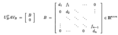
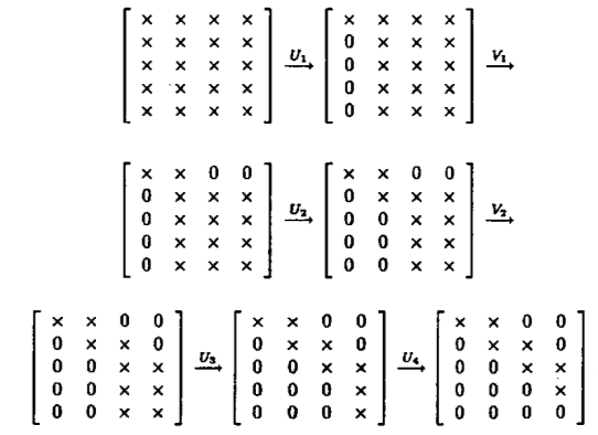 * **Golub-Kahan-Reinsch algorithm**:
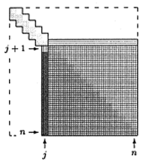
* Stage 1: Transform $\mathbf{A}$ to an upper bidiagonal form $\mathbf{B}$ (by Householder).
* Stage 2: Apply implicit-shift QR iteration to the tridiagonal matrix $\mathbf{B}^T \mathbf{B}$ _implicitly_.
* See Section 8.6 of [Matrix Computation](http://catalog.library.ucla.edu/vwebv/holdingsInfo?bibId=7122088) by Gene Golub and Charles Van Loan (2013) for more details.
* $4m^2 n + 8mn^2 + 9n^3$ flops for a tall $(m \ge n)$ matrix.
### Example
Julia functions: [`svd`](https://docs.julialang.org/en/v1/stdlib/LinearAlgebra/#LinearAlgebra.svd), [`svd!`](https://docs.julialang.org/en/v1/stdlib/LinearAlgebra/#LinearAlgebra.svd), [`svdvals`](https://docs.julialang.org/en/v1/stdlib/LinearAlgebra/#LinearAlgebra.svdvals), [`svdvals!`](https://docs.julialang.org/en/v1/stdlib/LinearAlgebra/#LinearAlgebra.svdvals!).
```{julia}
Random.seed!(123)
A = randn(5, 3)
Asvd = svd(A)
```
```{julia}
Asvd.U
```
```{julia}
# Vt is cheaper to extract than V
Asvd.Vt
```
```{julia}
Asvd.V
```
```{julia}
Asvd.S
```
**Don't request singular vectors unless needed.**
```{julia}
Random.seed!(123)
n, p = 1000, 500
A = randn(n, p)
@benchmark svdvals(A)
```
```{julia}
@benchmark svd(A)
```
## Lanczos/Arnoldi iterative method for top eigen-pairs
* Consider the Google PageRank problem. We want to find the top left eigenvector of the transition matrix $\mathbf{P}$. Direct methods such as (unsymmetric) QR or SVD takes forever. Iterative methods such as power method is feasible. However power method may take a large number of iterations.
* **Krylov subspace methods** are the state-of-art iterative methods for obtaining the top eigen-values/vectors or singular values/vectors of large **sparse** or **structured** matrices.
* **Lanczos method**: top eigen-pairs of a large _symmetric_ matrix.
* **Arnoldi method**: top eigen-pairs of a large _asymmetric_ matrix.
* Both methods are also adapted to obtain top singular values/vectors of large sparse or structured matrices.
* `eigs` and `svds` in Julia [Arpack.jl](https://github.com/JuliaLinearAlgebra/Arpack.jl) package and Matlab are wrappers of the ARPACK package, which implements Lanczos and Arnoldi methods.
```{julia}
using MatrixDepot, SparseArrays
# Download the Boeing/bcsstk38 matrix (sparse, pd, 8032-by-8032) from SuiteSparse collection
# https://www.cise.ufl.edu/research/sparse/matrices/Boeing/bcsstk38.html
A = matrixdepot("Boeing/bcsstk38")
# Change type of A from Symmetric{Float64,SparseMatrixCSC{Float64,Int64}} to SparseMatrixCSC
A = sparse(A)
@show typeof(A)
Afull = Matrix(A)
@show typeof(Afull)
# actual sparsity level
count(!iszero, A) / length(A)
```
```{julia}
using UnicodePlots
spy(A)
```
```{julia}
# top 5 eigenvalues by LAPACK (QR algorithm)
n = size(A, 1)
@time eigvals(Symmetric(Afull), (n-4):n)
```
```{julia}
using Arpack
# top 5 eigenvalues by iterative methods
@time eigs(A; nev=5, ritzvec=false, which=:LM)
```
```{julia}
@benchmark eigs($A; nev=5, ritzvec=false, which=:LM)
```
We see >1000 fold speedup in this case.
## Jacobi method for symmetric eigen-decomposition
Assume $\mathbf{A} \in \mathbf{R}^{n \times n}$ is symmetric and we seek the eigen-decomposition $\mathbf{A} = \mathbf{U} \Lambda \mathbf{U}^T$.
* Idea: Systematically reduce off-diagonal entries
$$
\text{off}(\mathbf{A}) = \sum_i \sum_{j \ne i} a_{ij}^2
$$
by Jacobi rotations.
* Jacobi/Givens rotations:
$$
\begin{eqnarray*}
\mathbf{J}(p,q,\theta) = \begin{pmatrix}
1 & & 0 & & 0 & & 0 \\
\vdots & \ddots & \vdots & & \vdots & & \vdots \\
0 & & \cos(\theta) & & \sin(\theta) & & 0 \\
\vdots & & \vdots & \ddots & \vdots & & \vdots \\
0 & & - \sin(\theta) & & \cos(\theta) & & 0 \\
\vdots & & \vdots & & \vdots & \ddots & \vdots \\
0 & & 0 & & 0 & & 1 \end{pmatrix},
\end{eqnarray*}
$$
$\mathbf{J}(p,q,\theta)$ is orthogonal.
* Consider $\mathbf{B} = \mathbf{J}^T \mathbf{A} \mathbf{J}$. $\mathbf{B}$ preserves the symmetry and eigenvalues of $\mathbf{A}$. Taking
$$
\begin{eqnarray*}
\begin{cases}
\tan (2\theta) = 2a_{pq}/({a_{qq}-a_{pp}}) & \text{if } a_{pp} \ne a_{qq} \\
\theta = \pi/4 & \text{if } a_{pp}=a_{qq}
\end{cases}
\end{eqnarray*}
$$
forces $b_{pq}=0$.
* Since orthogonal transform preserves Frobenius norm, we have
$$
b_{pp}^2 + b_{qq}^2 = a_{pp}^2 + a_{qq}^2 + 2a_{pq}^2.
$$
(Just check the 2-by-2 block)
* Since $\|\mathbf{A}\|_{\text{F}} = \|\mathbf{B}\|_{\text{F}}$, this implies that the off-diagonal part
$$
\text{off}(\mathbf{B}) = \text{off}(\mathbf{A}) - 2a_{pq}^2
$$
is decreased whenever $a_{pq} \ne 0$.
* One Jacobi rotation costs $O(n)$ flops.
* **Classical Jacobi**: search for the largest $|a_{ij}|$ at each iteration. $O(n^2)$ efforts!
* $\text{off}(\mathbf{A}) \le n(n-1) a_{ij}^2$ and $\text{off}(\mathbf{B}) = \text{off}(\mathbf{A}) - 2 a_{ij}^2$ together implies
$$
\text{off}(\mathbf{B}) \le \left( 1 - \frac{2}{n(n-1)} \right) \text{off}(\mathbf{A}).
$$
Thus Jacobi method converges in $O(n^2)$ iterations.
* In practice, cyclic-by-row implementation, to avoid the costly $O(n^2)$ search in the classical Jacobi.
* Jacobi method attracts a lot recent attention because of its rich inherent parallelism.
* **Parallel Jacobi**: "merry-go-round" to generate parallel ordering.
* **Golub-Kahan-Reinsch algorithm**:
* Stage 1: Transform $\mathbf{A}$ to an upper bidiagonal form $\mathbf{B}$ (by Householder).
* Stage 2: Apply implicit-shift QR iteration to the tridiagonal matrix $\mathbf{B}^T \mathbf{B}$ _implicitly_.
* See Section 8.6 of [Matrix Computation](http://catalog.library.ucla.edu/vwebv/holdingsInfo?bibId=7122088) by Gene Golub and Charles Van Loan (2013) for more details.
* $4m^2 n + 8mn^2 + 9n^3$ flops for a tall $(m \ge n)$ matrix.
### Example
Julia functions: [`svd`](https://docs.julialang.org/en/v1/stdlib/LinearAlgebra/#LinearAlgebra.svd), [`svd!`](https://docs.julialang.org/en/v1/stdlib/LinearAlgebra/#LinearAlgebra.svd), [`svdvals`](https://docs.julialang.org/en/v1/stdlib/LinearAlgebra/#LinearAlgebra.svdvals), [`svdvals!`](https://docs.julialang.org/en/v1/stdlib/LinearAlgebra/#LinearAlgebra.svdvals!).
```{julia}
Random.seed!(123)
A = randn(5, 3)
Asvd = svd(A)
```
```{julia}
Asvd.U
```
```{julia}
# Vt is cheaper to extract than V
Asvd.Vt
```
```{julia}
Asvd.V
```
```{julia}
Asvd.S
```
**Don't request singular vectors unless needed.**
```{julia}
Random.seed!(123)
n, p = 1000, 500
A = randn(n, p)
@benchmark svdvals(A)
```
```{julia}
@benchmark svd(A)
```
## Lanczos/Arnoldi iterative method for top eigen-pairs
* Consider the Google PageRank problem. We want to find the top left eigenvector of the transition matrix $\mathbf{P}$. Direct methods such as (unsymmetric) QR or SVD takes forever. Iterative methods such as power method is feasible. However power method may take a large number of iterations.
* **Krylov subspace methods** are the state-of-art iterative methods for obtaining the top eigen-values/vectors or singular values/vectors of large **sparse** or **structured** matrices.
* **Lanczos method**: top eigen-pairs of a large _symmetric_ matrix.
* **Arnoldi method**: top eigen-pairs of a large _asymmetric_ matrix.
* Both methods are also adapted to obtain top singular values/vectors of large sparse or structured matrices.
* `eigs` and `svds` in Julia [Arpack.jl](https://github.com/JuliaLinearAlgebra/Arpack.jl) package and Matlab are wrappers of the ARPACK package, which implements Lanczos and Arnoldi methods.
```{julia}
using MatrixDepot, SparseArrays
# Download the Boeing/bcsstk38 matrix (sparse, pd, 8032-by-8032) from SuiteSparse collection
# https://www.cise.ufl.edu/research/sparse/matrices/Boeing/bcsstk38.html
A = matrixdepot("Boeing/bcsstk38")
# Change type of A from Symmetric{Float64,SparseMatrixCSC{Float64,Int64}} to SparseMatrixCSC
A = sparse(A)
@show typeof(A)
Afull = Matrix(A)
@show typeof(Afull)
# actual sparsity level
count(!iszero, A) / length(A)
```
```{julia}
using UnicodePlots
spy(A)
```
```{julia}
# top 5 eigenvalues by LAPACK (QR algorithm)
n = size(A, 1)
@time eigvals(Symmetric(Afull), (n-4):n)
```
```{julia}
using Arpack
# top 5 eigenvalues by iterative methods
@time eigs(A; nev=5, ritzvec=false, which=:LM)
```
```{julia}
@benchmark eigs($A; nev=5, ritzvec=false, which=:LM)
```
We see >1000 fold speedup in this case.
## Jacobi method for symmetric eigen-decomposition
Assume $\mathbf{A} \in \mathbf{R}^{n \times n}$ is symmetric and we seek the eigen-decomposition $\mathbf{A} = \mathbf{U} \Lambda \mathbf{U}^T$.
* Idea: Systematically reduce off-diagonal entries
$$
\text{off}(\mathbf{A}) = \sum_i \sum_{j \ne i} a_{ij}^2
$$
by Jacobi rotations.
* Jacobi/Givens rotations:
$$
\begin{eqnarray*}
\mathbf{J}(p,q,\theta) = \begin{pmatrix}
1 & & 0 & & 0 & & 0 \\
\vdots & \ddots & \vdots & & \vdots & & \vdots \\
0 & & \cos(\theta) & & \sin(\theta) & & 0 \\
\vdots & & \vdots & \ddots & \vdots & & \vdots \\
0 & & - \sin(\theta) & & \cos(\theta) & & 0 \\
\vdots & & \vdots & & \vdots & \ddots & \vdots \\
0 & & 0 & & 0 & & 1 \end{pmatrix},
\end{eqnarray*}
$$
$\mathbf{J}(p,q,\theta)$ is orthogonal.
* Consider $\mathbf{B} = \mathbf{J}^T \mathbf{A} \mathbf{J}$. $\mathbf{B}$ preserves the symmetry and eigenvalues of $\mathbf{A}$. Taking
$$
\begin{eqnarray*}
\begin{cases}
\tan (2\theta) = 2a_{pq}/({a_{qq}-a_{pp}}) & \text{if } a_{pp} \ne a_{qq} \\
\theta = \pi/4 & \text{if } a_{pp}=a_{qq}
\end{cases}
\end{eqnarray*}
$$
forces $b_{pq}=0$.
* Since orthogonal transform preserves Frobenius norm, we have
$$
b_{pp}^2 + b_{qq}^2 = a_{pp}^2 + a_{qq}^2 + 2a_{pq}^2.
$$
(Just check the 2-by-2 block)
* Since $\|\mathbf{A}\|_{\text{F}} = \|\mathbf{B}\|_{\text{F}}$, this implies that the off-diagonal part
$$
\text{off}(\mathbf{B}) = \text{off}(\mathbf{A}) - 2a_{pq}^2
$$
is decreased whenever $a_{pq} \ne 0$.
* One Jacobi rotation costs $O(n)$ flops.
* **Classical Jacobi**: search for the largest $|a_{ij}|$ at each iteration. $O(n^2)$ efforts!
* $\text{off}(\mathbf{A}) \le n(n-1) a_{ij}^2$ and $\text{off}(\mathbf{B}) = \text{off}(\mathbf{A}) - 2 a_{ij}^2$ together implies
$$
\text{off}(\mathbf{B}) \le \left( 1 - \frac{2}{n(n-1)} \right) \text{off}(\mathbf{A}).
$$
Thus Jacobi method converges in $O(n^2)$ iterations.
* In practice, cyclic-by-row implementation, to avoid the costly $O(n^2)$ search in the classical Jacobi.
* Jacobi method attracts a lot recent attention because of its rich inherent parallelism.
* **Parallel Jacobi**: "merry-go-round" to generate parallel ordering.
