---
title: EM Algorithm (KL Chapter 13)
subtitle: Biostat/Biomath M257
author: Dr. Hua Zhou @ UCLA
date: today
format:
html:
theme: cosmo
embed-resources: true
number-sections: true
toc: true
toc-depth: 4
toc-location: left
code-fold: false
jupyter:
jupytext:
formats: 'ipynb,qmd'
text_representation:
extension: .qmd
format_name: quarto
format_version: '1.0'
jupytext_version: 1.14.5
kernelspec:
display_name: Julia 1.9.0
language: julia
name: julia-1.9
---
## Which statistical papers are most cited?
| Paper | Citations (5/10/2022) | Per Year |
|------------------------------------------|-----------:|----------:|
| FDR ([Benjamini and Hochberg, 1995](https://scholar.google.com/scholar?q=Controlling+the+false+discovery+rate)) | 85002 | **3148** |
| EM algorithm ([Dempster et al., 1977](https://scholar.google.com/scholar?q=Maximum+likelihood+from+incomplete+data+via+the+EM+algorithm&hl=en)) | 66596 | **1480** |
| Kaplan-Meier ([Kaplan and Meier, 1958](https://scholar.google.com/scholar?q=Nonparametric+estimation+from+incomplete+observations&hl=en)) | 62107 | 970 |
| Cox model ([Cox, 1972](https://scholar.google.com/scholar?q=Regression+models+and+life-tables&hl=en)) | 57383 | **1148** |
| Metropolis algorithm ([Metropolis et al., 1953](https://scholar.google.com/scholar?q=Equation+of+state+calculations+by+fast+computing+machines)) | 47851 | 694 |
| Lasso ([Tibshrani, 1996](https://scholar.google.com/scholar?q=Regression+shrinkage+and+selection+via+the+lasso)) | 46220 | **1778** |
| Unit root test ([Dickey and Fuller, 1979](https://scholar.google.com/scholar?q=Distribution+of+the+estimators+for+autoregressive+time+series+with+a+unit+root)) | 33783 | 786 |
| Compressed sensing ([Donoho, 2004](https://scholar.google.com/scholar?hl=en&as_sdt=0%2C5&q=compressed+sensing&btnG=)) | 30714 | **1706** |
| Propensity score ([Rosenbaum and Rubin, 1983](https://scholar.google.com/scholar?hl=en&as_sdt=0%2C5&q=rosenbaum+rubin+1983&btnG=)) | 31926 | 819 |
| Bootstrap ([Efron, 1979](https://scholar.google.com/scholar?q=Bootstrap+methods%3A+another+look+at+the+jackknife)) | 22789 | 530 |
| FFT ([Cooley and Tukey, 1965](https://scholar.google.com/scholar?q=An+algorithm+for+the+machine+calculation+of+complex+Fourier+series)) | 17817 | 313 |
| Inference and missing data ([Rubin, 1976](https://scholar.google.com/scholar?hl=en&as_sdt=0%2C5&q=Inference+and+missing+data&btnG=)) | 11672 | 254 |
| Gibbs sampler ([Gelfand and Smith, 1990](https://scholar.google.com/scholar?q=Sampling-based+approaches+to+calculating+marginal+densities)) | 9334 | 292 |
* Citation counts from Google Scholar on May 10, 2022.
* EM is one of the most influential statistical ideas, finding applications in various branches of science.
* History: Landmark paper [Dempster et al., 1977](https://scholar.google.com/scholar?q=Maximum+likelihood+from+incomplete+data+via+the+EM+algorithm&hl=en) on EM algorithm. Same idea appears in parameter estimation in HMM (Baum-Welch algorithm) by [Baum et al., 1970](http://www.jstor.org/stable/2239727?seq=1#page_scan_tab_contents).
## EM algorithm
* Goal: maximize the log-likelihood of the observed data $\ln g(\mathbf{y}|\theta)$ (optimization!)
* Notations:
* $\mathbf{Y}$: observed data
* $\mathbf{Z}$: missing data
* Idea: choose missing $\mathbf{Z}$ such that MLE for the complete data is easy.
* Let $f(\mathbf{y},\mathbf{z} | \theta)$ be the density of complete data.
* Iterative two-step procedure
* **E step**: calculate the conditional expectation
$$
Q(\theta|\theta^{(t)}) = \mathbf{E}_{\mathbf{Z}|\mathbf{Y}=\mathbf{y},\theta^{(t)}} [ \ln f(\mathbf{Y},\mathbf{Z}|\theta) \mid \mathbf{Y} = \mathbf{y}, \theta^{(t)}]
$$
* **M step**: maximize $Q(\theta|\theta^{(t)})$ to generate the next iterate
$$
\theta^{(t+1)} = \text{argmax}_{\theta} \, Q(\theta|\theta^{(t)})
$$
* (**Ascent property** of EM algorithm) By the information inequality,
$$
\begin{eqnarray*}
& & Q(\theta \mid \theta^{(t)}) - \ln g(\mathbf{y}|\theta) \\
&=& \mathbf{E} [\ln f(\mathbf{Y},\mathbf{Z}|\theta) | \mathbf{Y} = \mathbf{y}, \theta^{(t)}] - \ln g(\mathbf{y}|\theta) \\
&=& \mathbf{E} \left\{ \ln \left[ \frac{f(\mathbf{Y}, \mathbf{Z} \mid \theta)}{g(\mathbf{Y} \mid \theta)} \right] \mid \mathbf{Y} = \mathbf{y}, \theta^{(t)} \right\} \\
&\le& \mathbf{E} \left\{ \ln \left[ \frac{f(\mathbf{Y}, \mathbf{Z} \mid \theta^{(t)})}{g(\mathbf{Y} \mid \theta^{(t)})} \right] \mid \mathbf{Y} = \mathbf{y}, \theta^{(t)} \right\} \\
&=& Q(\theta^{(t)} \mid \theta^{(t)}) - \ln g(\mathbf{y} |\theta^{(t)}).
\end{eqnarray*}
$$
Rearranging shows that (**fundamental inequality of EM**)
$$
\begin{eqnarray*}
\ln g(\mathbf{y} \mid \theta) \ge Q(\theta \mid \theta^{(t)}) - Q(\theta^{(t)} \mid \theta^{(t)}) + \ln g(\mathbf{y} \mid \theta^{(t)})
\end{eqnarray*}
$$
for all $\theta$; in particular
$$
\begin{eqnarray*}
\ln g(\mathbf{y} \mid \theta^{(t+1)}) &\ge& Q(\theta^{(t+1)} \mid \theta^{(t)}) - Q(\theta^{(t)} \mid \theta^{(t)}) + \ln g(\mathbf{y} \mid \theta^{(t)}) \\
&\ge& \ln g(\mathbf{y} \mid \theta^{(t)}).
\end{eqnarray*}
$$
Obviously we only need
$$
Q(\theta^{(t+1)} \mid \theta^{(t)}) - Q(\theta^{(t)} \mid \theta^{(t)}) \ge 0
$$
for this ascent property to hold (**generalized EM**).
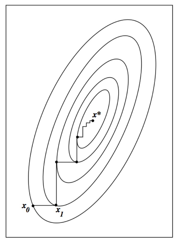
* Intuition? Keep these pictures in mind
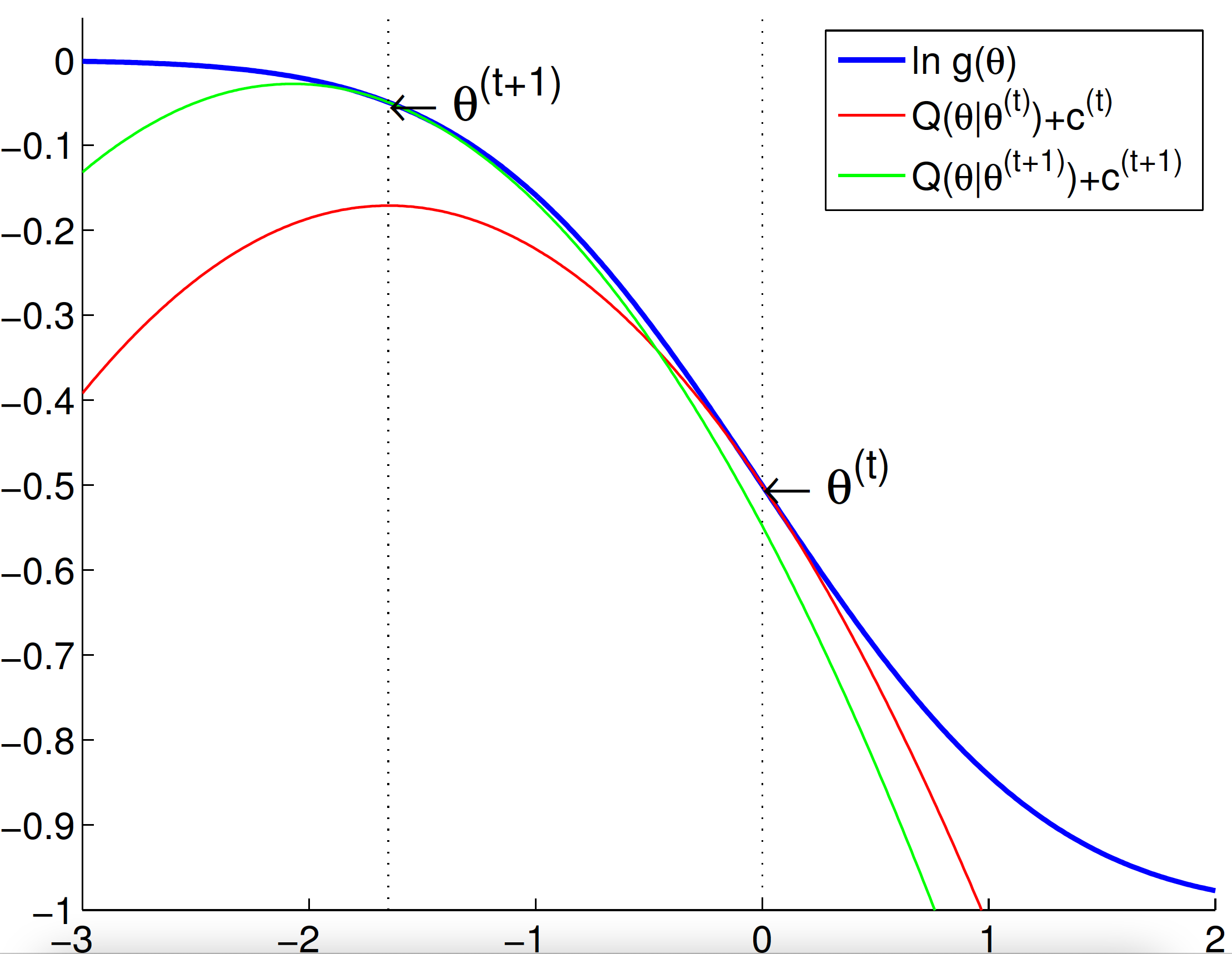
 * Under mild conditions, $\theta^{(t)}$ converges to a stationary point of $\ln g(\mathbf{y} \mid \theta)$.
* Numerous applications of EM:
finite mixture model, HMM (Baum-Welch algorithm), factor analysis, variance components model aka linear mixed model (LMM), hyper-parameter estimation in empirical Bayes procedure $\max_{\alpha} \int f(\mathbf{y}|\theta) \pi(\theta|\alpha) \, d \theta$, missing data, group/censorized/truncated model, ...
See Chapters 13 of [Numerical Analysis for Statisticians](http://ucla.worldcat.org/title/numerical-analysis-for-statisticians/oclc/793808354&referer=brief_results) by Kenneth Lange (2010) for more applications of EM.
## A canonical EM example: finite mixture models
* Under mild conditions, $\theta^{(t)}$ converges to a stationary point of $\ln g(\mathbf{y} \mid \theta)$.
* Numerous applications of EM:
finite mixture model, HMM (Baum-Welch algorithm), factor analysis, variance components model aka linear mixed model (LMM), hyper-parameter estimation in empirical Bayes procedure $\max_{\alpha} \int f(\mathbf{y}|\theta) \pi(\theta|\alpha) \, d \theta$, missing data, group/censorized/truncated model, ...
See Chapters 13 of [Numerical Analysis for Statisticians](http://ucla.worldcat.org/title/numerical-analysis-for-statisticians/oclc/793808354&referer=brief_results) by Kenneth Lange (2010) for more applications of EM.
## A canonical EM example: finite mixture models
 * Consider Gaussian finite mixture models with density
$$
h(\mathbf{y}) = \sum_{j=1}^k \pi_j h_j(\mathbf{y} \mid \mu_j, \Omega_j), \quad \mathbf{y} \in \mathbf{R}^{d},
$$
where
$$
h_j(\mathbf{y} \mid \mu_j, \Omega_j) = \left( \frac{1}{2\pi} \right)^{d/2} \det(\Omega_j)^{-1/2} e^{- \frac 12 (\mathbf{y} - \mu_j)^T \Omega_j^{-1} (\mathbf{y} - \mu_j)}
$$
are densities of multivariate normals $N_d(\mu_j, \Omega_j)$.
* Given iid data points $\mathbf{y}_1,\ldots,\mathbf{y}_n$, want to estimate parameters
$$
\theta = (\pi_1, \ldots, \pi_k, \mu_1, \ldots, \mu_k, \Omega_1,\ldots,\Omega_k)
$$
subject to constraint $\pi_j \ge 0, \sum_{j=1}^d \pi_j = 1, \Omega_j \succeq \mathbf{0}$.
* (Incomplete) data log-likelihood is
\begin{eqnarray*}
\ln g(\mathbf{y}_1,\ldots,\mathbf{y}_n|\theta) &=& \sum_{i=1}^n \ln h(\mathbf{y}_i) = \sum_{i=1}^n \ln \sum_{j=1}^k \pi_j h_j(\mathbf{y}_i \mid \mu_j, \Omega_j) \\
&=& \sum_{i=1}^n \ln \left[ \sum_{j=1}^k \pi_j \left( \frac{1}{2\pi} \right)^{d/2} \det(\Omega_j)^{-1/2} e^{- \frac 12 (\mathbf{y}_i - \mu_j)^T \Omega_j^{-1} (\mathbf{y}_i - \mu_j)} \right].
\end{eqnarray*}
* Let $z_{ij} = I \{\mathbf{y}_i$ comes from group $j \}$ be the missing data. The complete data likelihood is
$$
\begin{eqnarray*}
f(\mathbf{y},\mathbf{z} | \theta) = \prod_{i=1}^n \prod_{j=1}^k [\pi_j h_j(\mathbf{y}_i|\mu_j,\Omega_j)]^{z_{ij}}
\end{eqnarray*}
$$
and thus the complete log-likelihood is
$$
\begin{eqnarray*}
\ln f(\mathbf{y},\mathbf{z} | \theta) = \sum_{i=1}^n \sum_{j=1}^k z_{ij} [\ln \pi_j + \ln h_j(\mathbf{y}_i|\mu_j,\Omega_j)].
\end{eqnarray*}
$$
* **E step**: need to evaluate conditional expectation
$$
\begin{eqnarray*}
& & Q(\theta|\theta^{(t)})
= \mathbf{E} \left\{ \sum_{i=1}^n \sum_{j=1}^k z_{ij} [\ln \pi_j + \ln h_j(\mathbf{y}_i|\mu_j,\Omega_j)] \mid \mathbf{Y}=\mathbf{y}, \pi^{(t)}, \mu_1^{(t)}, \ldots, \mu_k^{(t)}, \Omega_1^{(t)}, \ldots, \Omega_k^{(t)} ] \right\}.
\end{eqnarray*}
$$
By Bayes rule, we have
$$
\begin{eqnarray*}
w_{ij}^{(t)} &:=& \mathbf{E} [z_{ij} \mid \mathbf{y}, \pi^{(t)}, \mu_1^{(t)}, \ldots, \mu_k^{(t)}, \Omega_1^{(t)}, \ldots, \Omega_k^{(t)}] \\
&=& \frac{\pi_j^{(t)} h_j(\mathbf{y}_i|\mu_j^{(t)},\Omega_j^{(t)})}{\sum_{j'=1}^k \pi_{j'}^{(t)} h_{j'}(\mathbf{y}_i|\mu_{j'}^{(t)},\Omega_{j'}^{(t)})}.
\end{eqnarray*}
$$
So the Q function becomes
$$
\begin{eqnarray*}
& & Q(\theta|\theta^{(t)})
= \sum_{i=1}^n \sum_{j=1}^k w_{ij}^{(t)} \ln \pi_j + \sum_{i=1}^n \sum_{j=1}^k w_{ij}^{(t)} \left[ - \frac{1}{2} \ln \det \Omega_j - \frac{1}{2} (\mathbf{y}_i - \mu_j)^T \Omega_j^{-1} (\mathbf{y}_i - \mu_j) \right].
\end{eqnarray*}
$$
* **M step**: maximizer of the Q function gives the next iterate
$$
\begin{eqnarray*}
\pi_j^{(t+1)} &=& \frac{\sum_i w_{ij}^{(t)}}{n} \\
\mu_j^{(t+1)} &=& \frac{\sum_{i=1}^n w_{ij}^{(t)} \mathbf{y}_i}{\sum_{i=1}^n w_{ij}^{(t)}} \\
\Omega_j^{(t+1)} &=& \frac{\sum_{i=1}^n w_{ij}^{(t)} (\mathbf{y}_i - \mu_j^{(t+1)}) (\mathbf{y}_i - \mu_j^{(t+1)})^T}{\sum_i w_{ij}^{(t)}}.
\end{eqnarray*}
$$
See KL Example 11.3.1 for multinomial MLE. See KL Example 11.2.3 for multivariate normal MLE.
* Compare these extremely simple updates to Newton type algorithms!
* Also note the ease of parallel computing with this EM algorithm. See, e.g.,
**Suchard, M. A.**; Wang, Q.; Chan, C.; Frelinger, J.; Cron, A.; West, M. Understanding GPU programming for statistical computation: studies in massively parallel massive mixtures. _Journal of Computational and Graphical Statistics_, 2010, 19, 419-438.
## Generalizations of EM - handle difficulties in M step
### Expectation Conditional Maximization (ECM)
* [Meng and Rubin (1993)](https://scholar.google.com/scholar?q=Maximum+likelihood+estimation+via+the+ECM+algorithm:+a+general+framework&hl=en&as_sdt=0&as_vis=1&oi=scholart).
* In some problems the M step is difficult (no analytic solution).
* Conditional maximization is easy (block ascent).
* partition parameter vector into blocks $\theta = (\theta_1, \ldots, \theta_B)$.
* alternately update $\theta_b$, $b=1,\ldots,B$.
* Consider Gaussian finite mixture models with density
$$
h(\mathbf{y}) = \sum_{j=1}^k \pi_j h_j(\mathbf{y} \mid \mu_j, \Omega_j), \quad \mathbf{y} \in \mathbf{R}^{d},
$$
where
$$
h_j(\mathbf{y} \mid \mu_j, \Omega_j) = \left( \frac{1}{2\pi} \right)^{d/2} \det(\Omega_j)^{-1/2} e^{- \frac 12 (\mathbf{y} - \mu_j)^T \Omega_j^{-1} (\mathbf{y} - \mu_j)}
$$
are densities of multivariate normals $N_d(\mu_j, \Omega_j)$.
* Given iid data points $\mathbf{y}_1,\ldots,\mathbf{y}_n$, want to estimate parameters
$$
\theta = (\pi_1, \ldots, \pi_k, \mu_1, \ldots, \mu_k, \Omega_1,\ldots,\Omega_k)
$$
subject to constraint $\pi_j \ge 0, \sum_{j=1}^d \pi_j = 1, \Omega_j \succeq \mathbf{0}$.
* (Incomplete) data log-likelihood is
\begin{eqnarray*}
\ln g(\mathbf{y}_1,\ldots,\mathbf{y}_n|\theta) &=& \sum_{i=1}^n \ln h(\mathbf{y}_i) = \sum_{i=1}^n \ln \sum_{j=1}^k \pi_j h_j(\mathbf{y}_i \mid \mu_j, \Omega_j) \\
&=& \sum_{i=1}^n \ln \left[ \sum_{j=1}^k \pi_j \left( \frac{1}{2\pi} \right)^{d/2} \det(\Omega_j)^{-1/2} e^{- \frac 12 (\mathbf{y}_i - \mu_j)^T \Omega_j^{-1} (\mathbf{y}_i - \mu_j)} \right].
\end{eqnarray*}
* Let $z_{ij} = I \{\mathbf{y}_i$ comes from group $j \}$ be the missing data. The complete data likelihood is
$$
\begin{eqnarray*}
f(\mathbf{y},\mathbf{z} | \theta) = \prod_{i=1}^n \prod_{j=1}^k [\pi_j h_j(\mathbf{y}_i|\mu_j,\Omega_j)]^{z_{ij}}
\end{eqnarray*}
$$
and thus the complete log-likelihood is
$$
\begin{eqnarray*}
\ln f(\mathbf{y},\mathbf{z} | \theta) = \sum_{i=1}^n \sum_{j=1}^k z_{ij} [\ln \pi_j + \ln h_j(\mathbf{y}_i|\mu_j,\Omega_j)].
\end{eqnarray*}
$$
* **E step**: need to evaluate conditional expectation
$$
\begin{eqnarray*}
& & Q(\theta|\theta^{(t)})
= \mathbf{E} \left\{ \sum_{i=1}^n \sum_{j=1}^k z_{ij} [\ln \pi_j + \ln h_j(\mathbf{y}_i|\mu_j,\Omega_j)] \mid \mathbf{Y}=\mathbf{y}, \pi^{(t)}, \mu_1^{(t)}, \ldots, \mu_k^{(t)}, \Omega_1^{(t)}, \ldots, \Omega_k^{(t)} ] \right\}.
\end{eqnarray*}
$$
By Bayes rule, we have
$$
\begin{eqnarray*}
w_{ij}^{(t)} &:=& \mathbf{E} [z_{ij} \mid \mathbf{y}, \pi^{(t)}, \mu_1^{(t)}, \ldots, \mu_k^{(t)}, \Omega_1^{(t)}, \ldots, \Omega_k^{(t)}] \\
&=& \frac{\pi_j^{(t)} h_j(\mathbf{y}_i|\mu_j^{(t)},\Omega_j^{(t)})}{\sum_{j'=1}^k \pi_{j'}^{(t)} h_{j'}(\mathbf{y}_i|\mu_{j'}^{(t)},\Omega_{j'}^{(t)})}.
\end{eqnarray*}
$$
So the Q function becomes
$$
\begin{eqnarray*}
& & Q(\theta|\theta^{(t)})
= \sum_{i=1}^n \sum_{j=1}^k w_{ij}^{(t)} \ln \pi_j + \sum_{i=1}^n \sum_{j=1}^k w_{ij}^{(t)} \left[ - \frac{1}{2} \ln \det \Omega_j - \frac{1}{2} (\mathbf{y}_i - \mu_j)^T \Omega_j^{-1} (\mathbf{y}_i - \mu_j) \right].
\end{eqnarray*}
$$
* **M step**: maximizer of the Q function gives the next iterate
$$
\begin{eqnarray*}
\pi_j^{(t+1)} &=& \frac{\sum_i w_{ij}^{(t)}}{n} \\
\mu_j^{(t+1)} &=& \frac{\sum_{i=1}^n w_{ij}^{(t)} \mathbf{y}_i}{\sum_{i=1}^n w_{ij}^{(t)}} \\
\Omega_j^{(t+1)} &=& \frac{\sum_{i=1}^n w_{ij}^{(t)} (\mathbf{y}_i - \mu_j^{(t+1)}) (\mathbf{y}_i - \mu_j^{(t+1)})^T}{\sum_i w_{ij}^{(t)}}.
\end{eqnarray*}
$$
See KL Example 11.3.1 for multinomial MLE. See KL Example 11.2.3 for multivariate normal MLE.
* Compare these extremely simple updates to Newton type algorithms!
* Also note the ease of parallel computing with this EM algorithm. See, e.g.,
**Suchard, M. A.**; Wang, Q.; Chan, C.; Frelinger, J.; Cron, A.; West, M. Understanding GPU programming for statistical computation: studies in massively parallel massive mixtures. _Journal of Computational and Graphical Statistics_, 2010, 19, 419-438.
## Generalizations of EM - handle difficulties in M step
### Expectation Conditional Maximization (ECM)
* [Meng and Rubin (1993)](https://scholar.google.com/scholar?q=Maximum+likelihood+estimation+via+the+ECM+algorithm:+a+general+framework&hl=en&as_sdt=0&as_vis=1&oi=scholart).
* In some problems the M step is difficult (no analytic solution).
* Conditional maximization is easy (block ascent).
* partition parameter vector into blocks $\theta = (\theta_1, \ldots, \theta_B)$.
* alternately update $\theta_b$, $b=1,\ldots,B$.
 * Ascent property still holds. Why?
* ECM may converge slower than EM (more iterations) but the total computer time may be shorter due to ease of the CM step.
### ECM Either (ECME)
* [Liu and Rubin (1994)](https://scholar.google.com/scholar?hl=en&as_sdt=0%2C5&as_vis=1&q=The+ECME+algorithm%3A+a+simple+extension+of+EM+and+ECM+with+faster+monotone+convergence&btnG=).
* Each CM step maximizes either the $Q$ function or the original incomplete observed log-likelihood.
* Ascent property still holds. Why?
* Faster convergence than ECM.
### Alternating ECM (AECM)
* [Meng and van Dyk (1997)](https://scholar.google.com/scholar?hl=en&as_sdt=0%2C5&q=The+EM+algorithm+an+old+folk-song+sung+to+a+fast+new+tune&btnG=).
* The specification of the complete-data is allowed to be different on each CM-step.
* Ascent property still holds. Why?
### PX-EM and efficient data augmentation
* Parameter-Expanded EM. [Liu, Rubin, and Wu (1998)](https://scholar.google.com/scholar?hl=en&as_sdt=0%2C5&q=Parameter+expansion+to+accelerate+EM%3A+the+px-em+algorithm&btnG=), [Liu and Wu (1999)](https://scholar.google.com/scholar?cluster=15342818142955984734&hl=en&as_sdt=0,5).
* Efficient data augmentation. [Meng and van Dyk (1997)](https://scholar.google.com/scholar?hl=en&as_sdt=0%2C5&q=The+EM+algorithm+an+old+folk-song+sung+to+a+fast+new+tune&btnG=).
* Idea: Speed up the convergence of EM algorithm by efficiently augmenting the observed data (introducing a working parameter in the specification of complete data).
### Example: t distribution
#### EM
* $\mathbf{W} \in \mathbb{R}^{p}$ is a multivariate $t$-distribution $t_p(\mu,\Sigma,\nu)$ if $\mathbf{W} \sim N(\mu, \Sigma/u)$ and $u \sim \text{gamma}\left(\frac{\nu}{2}, \frac{\nu}{2}\right)$.
* Widely used for robust modeling.
* Recall Gamma($\alpha,\beta$) has density
\begin{eqnarray*}
f(u \mid \alpha,\beta) = \frac{\beta^{\alpha} u^{\alpha-1}}{\Gamma(\alpha)} e^{-\beta u}, \quad u \ge 0,
\end{eqnarray*}
with mean $\mathbf{E}(U)=\alpha/\beta$, and $\mathbf{E}(\log U) = \psi(\alpha) - \log \beta$.
* Density of $\mathbf{W}$ is
\begin{eqnarray*}
f_p(\mathbf{w} \mid \mu, \Sigma, \nu) = \frac{\Gamma \left(\frac{\nu+p}{2}\right) \text{det}(\Sigma)^{-1/2}}{(\pi \nu)^{p/2} \Gamma(\nu/2) [1 + \delta (\mathbf{w},\mu;\Sigma)/\nu]^{(\nu+p)/2}},
\end{eqnarray*}
where
\begin{eqnarray*}
\delta (\mathbf{w},\mu;\Sigma) = (\mathbf{w} - \mu)^T \Sigma^{-1} (\mathbf{w} - \mu)
\end{eqnarray*}
is the Mahalanobis squared distance between $\mathbf{w}$ and $\mu$.
* Given iid data $\mathbf{w}_1, \ldots, \mathbf{w}_n$, the log-likelihood is
\begin{eqnarray*}
L(\mu, \Sigma, \nu) &=& - \frac{np}{2} \log (\pi \nu) + n \left[ \log \Gamma \left(\frac{\nu+p}{2}\right) - \log \Gamma \left(\frac{\nu}{2}\right) \right] \\
&& - \frac n2 \log \det \Sigma + \frac n2 (\nu + p) \log \nu \\
&& - \frac{\nu + p}{2} \sum_{j=1}^n \log [\nu + \delta (\mathbf{w}_j,\mu;\Sigma) ]
\end{eqnarray*}
How to compute the MLE $(\hat \mu, \hat \Sigma, \hat \nu)$?
* $\mathbf{W}_j | u_j$ independent $N(\mu,\Sigma/u_j)$ and $U_j$ iid gamma $\left(\frac{\nu}{2},\frac{\nu}{2}\right)$.
* Missing data: $\mathbf{z}=(u_1,\ldots,u_n)^T$.
* Log-likelihood of complete data is
\begin{eqnarray*}
L_c (\mu, \Sigma, \nu) &=& - \frac{np}{2} \ln (2\pi) - \frac{n}{2} \log \det \Sigma \\
& & - \frac 12 \sum_{j=1}^n u_j (\mathbf{w}_j - \mu)^T \Sigma^{-1} (\mathbf{w}_j - \mu) \\
& & - n \log \Gamma \left(\frac{\nu}{2}\right) + \frac{n \nu}{2} \log \left(\frac{\nu}{2}\right) \\
& & + \frac{\nu}{2} \sum_{j=1}^n (\log u_j - u_j) - \sum_{j=1}^n \log u_j.
\end{eqnarray*}
* Since gamma is the conjugate prior for normal-gamma model, conditional distribution of $U$ given $\mathbf{W} = \mathbf{w}$ is gamma$((\nu+p)/2, (\nu + \delta(\mathbf{w},\mu; \Sigma))/2)$. Thus
\begin{eqnarray*}
\mathbf{E} (U_j \mid \mathbf{w}_j, \mu^{(t)},\Sigma^{(t)},\nu^{(t)}) &=& \frac{\nu^{(t)} + p}{\nu^{(t)} + \delta(\mathbf{w}_j,\mu^{(t)};\Sigma^{(t)})} =: u_j^{(t)} \\
\mathbf{E} (\log U_j \mid \mathbf{w}_j, \mu^{(t)},\Sigma^{(t)},\nu^{(t)}) &=& \log u_j^{(t)} + \left[ \psi \left(\frac{\nu^{(t)}+p}{2}\right) - \log \left(\frac{\nu^{(t)}+p}{2}\right) \right].
\end{eqnarray*}
* Overall $Q$ function (up to an additive constant) takes the form
\begin{eqnarray*}
%Q(\mubf,\Sigmabf,\nu \mid \mubf^{(t)},\Sigmabf^{(t)},\nu^{(t)}) =
& & - \frac n2 \log \det \Sigma - \frac 12 \sum_{j=1}^n u_j^{(t)} (\mathbf{w}_j - \mu)^T \Sigma^{-1} (\mathbf{w}_j - \mu) \\
& & - n \log \Gamma \left(\frac{\nu}{2}\right) + \frac{n \nu}{2} \log \left(\frac{\nu}{2}\right) \\
& & + \frac{n \nu}{2} \left[ \frac 1n \sum_{j=1}^n \left(\log u_j^{(t)} - u_j^{(t)}\right) + \psi\left(\frac{\nu^{(t)}+p}{2}\right) - \log \left(\frac{\nu^{(t)}+p}{2}\right) \right].
\end{eqnarray*}
* Maximization over $(\mu, \Sigma)$ is simply a weighted multivariate normal problem
\begin{eqnarray*}
\mu^{(t+1)} &=& \frac{\sum_{j=1}^n u_j^{(t)} \mathbf{w}_j}{\sum_{j=1}^n u_j^{(t)}} \\
\Sigma^{(t+1)} &=& \frac 1n \sum_{j=1}^n u_j^{(t)} (\mathbf{w}_j - \mu^{(t+1)}) (\mathbf{w}_j - \mu^{(t+1)})^T.
\end{eqnarray*}
Notice down-weighting of outliers is obvious in the update.
* Maximization over $\nu$ is a univariate problem - Brent method, golden section, or bisection.
#### ECM and ECME
Partition parameter $(\mu,\Sigma,\nu)$ into two blocks $(\mu,\Sigma)$ and $\nu$:
* ECM = EM for this example. Why?
* ECME: In the second CM step, maximize over $\nu$ in terms of the original log-likelihood function instead of the $Q$ function. They have similar difficulty since both are univariate optimization problems!
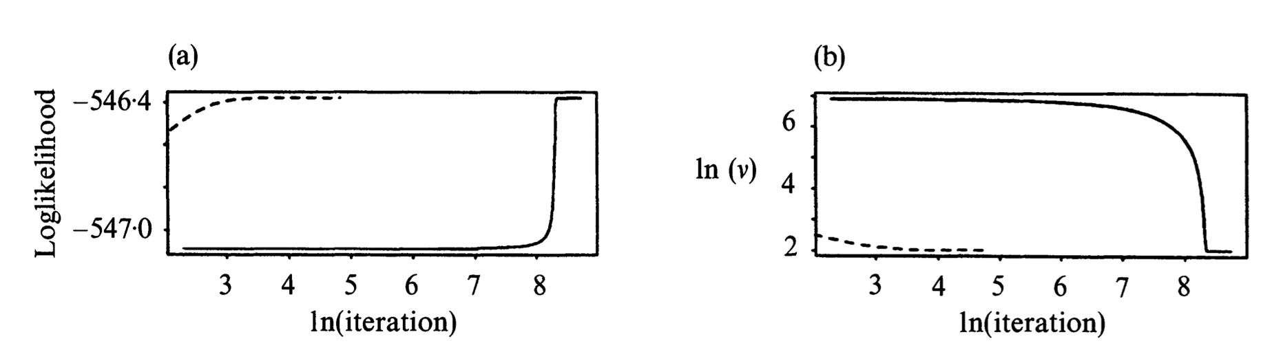
* An example from [Liu and Rubin (1994)](https://scholar.google.com/scholar?hl=en&as_sdt=0%2C5&as_vis=1&q=The+ECME+algorithm%3A+a+simple+extension+of+EM+and+ECM+with+faster+monotone+convergence&btnG=). $n=79$, $p=2$, with missing entries. EM=ECM: solid line. ECME: dashed line.
* Ascent property still holds. Why?
* ECM may converge slower than EM (more iterations) but the total computer time may be shorter due to ease of the CM step.
### ECM Either (ECME)
* [Liu and Rubin (1994)](https://scholar.google.com/scholar?hl=en&as_sdt=0%2C5&as_vis=1&q=The+ECME+algorithm%3A+a+simple+extension+of+EM+and+ECM+with+faster+monotone+convergence&btnG=).
* Each CM step maximizes either the $Q$ function or the original incomplete observed log-likelihood.
* Ascent property still holds. Why?
* Faster convergence than ECM.
### Alternating ECM (AECM)
* [Meng and van Dyk (1997)](https://scholar.google.com/scholar?hl=en&as_sdt=0%2C5&q=The+EM+algorithm+an+old+folk-song+sung+to+a+fast+new+tune&btnG=).
* The specification of the complete-data is allowed to be different on each CM-step.
* Ascent property still holds. Why?
### PX-EM and efficient data augmentation
* Parameter-Expanded EM. [Liu, Rubin, and Wu (1998)](https://scholar.google.com/scholar?hl=en&as_sdt=0%2C5&q=Parameter+expansion+to+accelerate+EM%3A+the+px-em+algorithm&btnG=), [Liu and Wu (1999)](https://scholar.google.com/scholar?cluster=15342818142955984734&hl=en&as_sdt=0,5).
* Efficient data augmentation. [Meng and van Dyk (1997)](https://scholar.google.com/scholar?hl=en&as_sdt=0%2C5&q=The+EM+algorithm+an+old+folk-song+sung+to+a+fast+new+tune&btnG=).
* Idea: Speed up the convergence of EM algorithm by efficiently augmenting the observed data (introducing a working parameter in the specification of complete data).
### Example: t distribution
#### EM
* $\mathbf{W} \in \mathbb{R}^{p}$ is a multivariate $t$-distribution $t_p(\mu,\Sigma,\nu)$ if $\mathbf{W} \sim N(\mu, \Sigma/u)$ and $u \sim \text{gamma}\left(\frac{\nu}{2}, \frac{\nu}{2}\right)$.
* Widely used for robust modeling.
* Recall Gamma($\alpha,\beta$) has density
\begin{eqnarray*}
f(u \mid \alpha,\beta) = \frac{\beta^{\alpha} u^{\alpha-1}}{\Gamma(\alpha)} e^{-\beta u}, \quad u \ge 0,
\end{eqnarray*}
with mean $\mathbf{E}(U)=\alpha/\beta$, and $\mathbf{E}(\log U) = \psi(\alpha) - \log \beta$.
* Density of $\mathbf{W}$ is
\begin{eqnarray*}
f_p(\mathbf{w} \mid \mu, \Sigma, \nu) = \frac{\Gamma \left(\frac{\nu+p}{2}\right) \text{det}(\Sigma)^{-1/2}}{(\pi \nu)^{p/2} \Gamma(\nu/2) [1 + \delta (\mathbf{w},\mu;\Sigma)/\nu]^{(\nu+p)/2}},
\end{eqnarray*}
where
\begin{eqnarray*}
\delta (\mathbf{w},\mu;\Sigma) = (\mathbf{w} - \mu)^T \Sigma^{-1} (\mathbf{w} - \mu)
\end{eqnarray*}
is the Mahalanobis squared distance between $\mathbf{w}$ and $\mu$.
* Given iid data $\mathbf{w}_1, \ldots, \mathbf{w}_n$, the log-likelihood is
\begin{eqnarray*}
L(\mu, \Sigma, \nu) &=& - \frac{np}{2} \log (\pi \nu) + n \left[ \log \Gamma \left(\frac{\nu+p}{2}\right) - \log \Gamma \left(\frac{\nu}{2}\right) \right] \\
&& - \frac n2 \log \det \Sigma + \frac n2 (\nu + p) \log \nu \\
&& - \frac{\nu + p}{2} \sum_{j=1}^n \log [\nu + \delta (\mathbf{w}_j,\mu;\Sigma) ]
\end{eqnarray*}
How to compute the MLE $(\hat \mu, \hat \Sigma, \hat \nu)$?
* $\mathbf{W}_j | u_j$ independent $N(\mu,\Sigma/u_j)$ and $U_j$ iid gamma $\left(\frac{\nu}{2},\frac{\nu}{2}\right)$.
* Missing data: $\mathbf{z}=(u_1,\ldots,u_n)^T$.
* Log-likelihood of complete data is
\begin{eqnarray*}
L_c (\mu, \Sigma, \nu) &=& - \frac{np}{2} \ln (2\pi) - \frac{n}{2} \log \det \Sigma \\
& & - \frac 12 \sum_{j=1}^n u_j (\mathbf{w}_j - \mu)^T \Sigma^{-1} (\mathbf{w}_j - \mu) \\
& & - n \log \Gamma \left(\frac{\nu}{2}\right) + \frac{n \nu}{2} \log \left(\frac{\nu}{2}\right) \\
& & + \frac{\nu}{2} \sum_{j=1}^n (\log u_j - u_j) - \sum_{j=1}^n \log u_j.
\end{eqnarray*}
* Since gamma is the conjugate prior for normal-gamma model, conditional distribution of $U$ given $\mathbf{W} = \mathbf{w}$ is gamma$((\nu+p)/2, (\nu + \delta(\mathbf{w},\mu; \Sigma))/2)$. Thus
\begin{eqnarray*}
\mathbf{E} (U_j \mid \mathbf{w}_j, \mu^{(t)},\Sigma^{(t)},\nu^{(t)}) &=& \frac{\nu^{(t)} + p}{\nu^{(t)} + \delta(\mathbf{w}_j,\mu^{(t)};\Sigma^{(t)})} =: u_j^{(t)} \\
\mathbf{E} (\log U_j \mid \mathbf{w}_j, \mu^{(t)},\Sigma^{(t)},\nu^{(t)}) &=& \log u_j^{(t)} + \left[ \psi \left(\frac{\nu^{(t)}+p}{2}\right) - \log \left(\frac{\nu^{(t)}+p}{2}\right) \right].
\end{eqnarray*}
* Overall $Q$ function (up to an additive constant) takes the form
\begin{eqnarray*}
%Q(\mubf,\Sigmabf,\nu \mid \mubf^{(t)},\Sigmabf^{(t)},\nu^{(t)}) =
& & - \frac n2 \log \det \Sigma - \frac 12 \sum_{j=1}^n u_j^{(t)} (\mathbf{w}_j - \mu)^T \Sigma^{-1} (\mathbf{w}_j - \mu) \\
& & - n \log \Gamma \left(\frac{\nu}{2}\right) + \frac{n \nu}{2} \log \left(\frac{\nu}{2}\right) \\
& & + \frac{n \nu}{2} \left[ \frac 1n \sum_{j=1}^n \left(\log u_j^{(t)} - u_j^{(t)}\right) + \psi\left(\frac{\nu^{(t)}+p}{2}\right) - \log \left(\frac{\nu^{(t)}+p}{2}\right) \right].
\end{eqnarray*}
* Maximization over $(\mu, \Sigma)$ is simply a weighted multivariate normal problem
\begin{eqnarray*}
\mu^{(t+1)} &=& \frac{\sum_{j=1}^n u_j^{(t)} \mathbf{w}_j}{\sum_{j=1}^n u_j^{(t)}} \\
\Sigma^{(t+1)} &=& \frac 1n \sum_{j=1}^n u_j^{(t)} (\mathbf{w}_j - \mu^{(t+1)}) (\mathbf{w}_j - \mu^{(t+1)})^T.
\end{eqnarray*}
Notice down-weighting of outliers is obvious in the update.
* Maximization over $\nu$ is a univariate problem - Brent method, golden section, or bisection.
#### ECM and ECME
Partition parameter $(\mu,\Sigma,\nu)$ into two blocks $(\mu,\Sigma)$ and $\nu$:
* ECM = EM for this example. Why?
* ECME: In the second CM step, maximize over $\nu$ in terms of the original log-likelihood function instead of the $Q$ function. They have similar difficulty since both are univariate optimization problems!
* An example from [Liu and Rubin (1994)](https://scholar.google.com/scholar?hl=en&as_sdt=0%2C5&as_vis=1&q=The+ECME+algorithm%3A+a+simple+extension+of+EM+and+ECM+with+faster+monotone+convergence&btnG=). $n=79$, $p=2$, with missing entries. EM=ECM: solid line. ECME: dashed line.
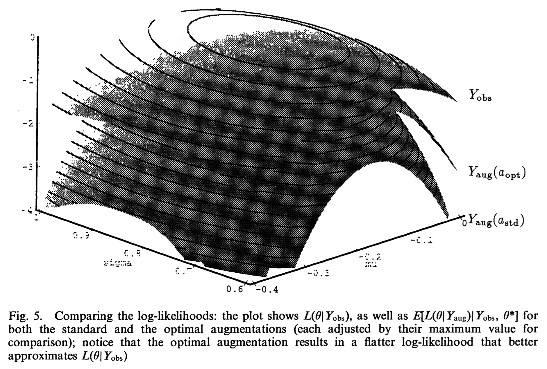
 #### Efficient data augmentation
Assume $\nu$ known:
* Write $\mathbf{W}_j = \mu + \mathbf{C}_j / U_j^{1/2}$, where $\mathbf{C}_j$ is $N(\mathbf{0},\Sigma)$ independent of $U_j$ which is gamma$\left(\frac{\nu}{2},\frac{\nu}{2}\right)$.
* $\mathbf{W}_j = \mu + \det (\Sigma)^{-a/2} \mathbf{C}_j / U_j^{1/2}(a)$, where $U_j(a) = \det(\Sigma)^{-a} U_j$.
* Then the complete data is $(\mathbf{w}, \mathbf{z}(a))$, $a$ the working parameter.
* $a=0$ corresponds to the vanilla EM.
* Meng and van Dyk (1997) recommend using $a_{\text{opt}} = 1/(\nu+p)$ to maximize the convergence rate.
* Exercise: work out the EM update for this special case.
* The only change to the vanilla EM is to replace the denominator $n$ in the update of $\Sigma$ by $\sum_{j=1}^n u_j^{(t)}$.
* PX-EM (Liu, Rubin, and Wu, 1998) leads to the same update.
#### Efficient data augmentation
Assume $\nu$ known:
* Write $\mathbf{W}_j = \mu + \mathbf{C}_j / U_j^{1/2}$, where $\mathbf{C}_j$ is $N(\mathbf{0},\Sigma)$ independent of $U_j$ which is gamma$\left(\frac{\nu}{2},\frac{\nu}{2}\right)$.
* $\mathbf{W}_j = \mu + \det (\Sigma)^{-a/2} \mathbf{C}_j / U_j^{1/2}(a)$, where $U_j(a) = \det(\Sigma)^{-a} U_j$.
* Then the complete data is $(\mathbf{w}, \mathbf{z}(a))$, $a$ the working parameter.
* $a=0$ corresponds to the vanilla EM.
* Meng and van Dyk (1997) recommend using $a_{\text{opt}} = 1/(\nu+p)$ to maximize the convergence rate.
* Exercise: work out the EM update for this special case.
* The only change to the vanilla EM is to replace the denominator $n$ in the update of $\Sigma$ by $\sum_{j=1}^n u_j^{(t)}$.
* PX-EM (Liu, Rubin, and Wu, 1998) leads to the same update.
 Assume $\nu$ unknown:
* Version 1: $a=a_{\text{opt}}$ in both updating of $(\mu,\Sigma)$ and $\nu$.
* Version 2: $a=a_{\text{opt}}$ for updating $(\mu,\Sigma)$ and taking the observed data as complete data for updating $\nu$.
Conclusion in Meng and van Dyk (1997): Version 1 is $8 \sim 12$ faster than EM=ECM or ECME. Version 2 is only slightly more efficient than Version 1
## Generalizations of EM - handle difficulties in E step
### Monte Carlo EM (MCEM)
* [Wei and Tanner (1990)](https://scholar.google.com/scholar?hl=en&as_sdt=0%2C5&q=A+Monte+Carlo+implementation+of+the+EM+algorithm+and+the+poor+man’s+data+augmentation+algorithms&btnG=).
* Hard to calculate $Q$ function? Simulate!
\begin{eqnarray*}
Q(\theta \mid \theta^{(t)}) \approx \frac 1m \sum_{j=1}^m \ln f(\mathbf{y}, \mathbf{z}_j \mid \theta),
\end{eqnarray*}
where $\mathbf{z}_j$ are iid from conditional distribution of missing data given $\mathbf{y}$ and previous iterate $\theta^{(t)}$.
* Ascent property may be lost due to Monte Carlo errors.
* Example: capture-recapture model, generalized linear mixed model (GLMM).
### Stochastic EM (SEM) and Simulated Annealing EM (SAEM)
SEM
* Celeux and Diebolt (1985).
* Same as MCEM with $m=1$. A single draw of missing data $\mathbf{z}$ from the conditional distribution.
* $\theta^{(t)}$ forms a Markov chain which converges to a stationary distribution. No definite relation between this stationary distribution and the MLE.
* In some specific cases, it can be shown that the stationary distribution concentrates around the MLE with a variance inversely proportional to the sample size.
* Advantage: can escape the attraction to inferior mode/saddle point in some mixture model problems.
SAEM
* Celeux and Deibolt (1989).
* Increase $m$ with the iterations, ending up with an EM algorithm.
### Data-augmentation (DA) algorithm
* [Tanner and Wong (1987)](https://scholar.google.com/scholar?q=The+calculation+of+posterior+distributions+by+data+augmentation&hl=en&as_sdt=0&as_vis=1&oi=scholart).
* Aim for sampling from $p(\theta|\mathbf{y})$ instead of maximization.
* Idea: incomplete data posterior density is complicated, but the complete-data posterior density is relatively easy to sample.
* Data augmentation algorithm:
* draw $\mathbf{z}^{(t+1)}$ conditional on $(\theta^{(t)},\mathbf{y})$
* draw $\theta^{(t+1)}$ conditional on $(\mathbf{z}^{(t+1)},\mathbf{y})$
* A special case of Gibbs sampler.
* $\theta^{(t)}$ converges to the distribution $p(\theta|\mathbf{y})$ under general conditions.
* Ergodic mean converges to the posterior mean $\mathbf{E}(\theta|\mathbf{y})$, which may perform better than MLE in finite sample.
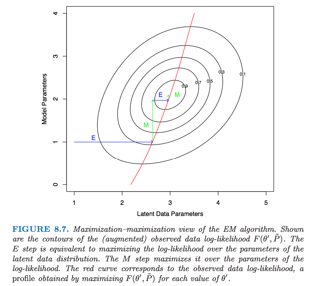
## EM as a maximization-maximization procedure
* [Neal and Hinton (1999)](https://doi.org/10.1007/978-94-011-5014-9_12).
* Consider the objective function
\begin{eqnarray*}
F(\theta, q) = \mathbf{E}_q [\ln f(\mathbf{Z},\mathbf{y} \mid \theta)] + H(q)
\end{eqnarray*}
over $\Theta \times {\cal Q}$, where ${\cal Q}$ is the set of all conditional pdfs of the missing data $\{q(\mathbf{z}) = p(\mathbf{z} \mid \mathbf{y}, \theta), \theta \in \Theta \}$ and $H(q) = -\mathbf{E}_q \log q$ is the entropy of $q$.
* EM is essentially performing coordinate ascent for maximizing $F$
* E step: At current iterate $\theta^{(t)}$,
\begin{eqnarray*}
F(\theta^{(t)}, q) = \mathbf{E}_q [\log p(\mathbf{Z} \mid \mathbf{y}, \theta^{(t)})] - \mathbf{E}_q \log q + \ln g(\mathbf{y} \mid \theta^{(t)}).
\end{eqnarray*}
The maximizing conditional pdf is given by $q = \log f(\mathbf{Z} \mid \mathbf{y}, \theta^{(t)})$
* M step: Substitute $q = \log f(\mathbf{Z} \mid \mathbf{y}, \theta^{(t)})$ into $F$ and maximize over $\theta$
Assume $\nu$ unknown:
* Version 1: $a=a_{\text{opt}}$ in both updating of $(\mu,\Sigma)$ and $\nu$.
* Version 2: $a=a_{\text{opt}}$ for updating $(\mu,\Sigma)$ and taking the observed data as complete data for updating $\nu$.
Conclusion in Meng and van Dyk (1997): Version 1 is $8 \sim 12$ faster than EM=ECM or ECME. Version 2 is only slightly more efficient than Version 1
## Generalizations of EM - handle difficulties in E step
### Monte Carlo EM (MCEM)
* [Wei and Tanner (1990)](https://scholar.google.com/scholar?hl=en&as_sdt=0%2C5&q=A+Monte+Carlo+implementation+of+the+EM+algorithm+and+the+poor+man’s+data+augmentation+algorithms&btnG=).
* Hard to calculate $Q$ function? Simulate!
\begin{eqnarray*}
Q(\theta \mid \theta^{(t)}) \approx \frac 1m \sum_{j=1}^m \ln f(\mathbf{y}, \mathbf{z}_j \mid \theta),
\end{eqnarray*}
where $\mathbf{z}_j$ are iid from conditional distribution of missing data given $\mathbf{y}$ and previous iterate $\theta^{(t)}$.
* Ascent property may be lost due to Monte Carlo errors.
* Example: capture-recapture model, generalized linear mixed model (GLMM).
### Stochastic EM (SEM) and Simulated Annealing EM (SAEM)
SEM
* Celeux and Diebolt (1985).
* Same as MCEM with $m=1$. A single draw of missing data $\mathbf{z}$ from the conditional distribution.
* $\theta^{(t)}$ forms a Markov chain which converges to a stationary distribution. No definite relation between this stationary distribution and the MLE.
* In some specific cases, it can be shown that the stationary distribution concentrates around the MLE with a variance inversely proportional to the sample size.
* Advantage: can escape the attraction to inferior mode/saddle point in some mixture model problems.
SAEM
* Celeux and Deibolt (1989).
* Increase $m$ with the iterations, ending up with an EM algorithm.
### Data-augmentation (DA) algorithm
* [Tanner and Wong (1987)](https://scholar.google.com/scholar?q=The+calculation+of+posterior+distributions+by+data+augmentation&hl=en&as_sdt=0&as_vis=1&oi=scholart).
* Aim for sampling from $p(\theta|\mathbf{y})$ instead of maximization.
* Idea: incomplete data posterior density is complicated, but the complete-data posterior density is relatively easy to sample.
* Data augmentation algorithm:
* draw $\mathbf{z}^{(t+1)}$ conditional on $(\theta^{(t)},\mathbf{y})$
* draw $\theta^{(t+1)}$ conditional on $(\mathbf{z}^{(t+1)},\mathbf{y})$
* A special case of Gibbs sampler.
* $\theta^{(t)}$ converges to the distribution $p(\theta|\mathbf{y})$ under general conditions.
* Ergodic mean converges to the posterior mean $\mathbf{E}(\theta|\mathbf{y})$, which may perform better than MLE in finite sample.
## EM as a maximization-maximization procedure
* [Neal and Hinton (1999)](https://doi.org/10.1007/978-94-011-5014-9_12).
* Consider the objective function
\begin{eqnarray*}
F(\theta, q) = \mathbf{E}_q [\ln f(\mathbf{Z},\mathbf{y} \mid \theta)] + H(q)
\end{eqnarray*}
over $\Theta \times {\cal Q}$, where ${\cal Q}$ is the set of all conditional pdfs of the missing data $\{q(\mathbf{z}) = p(\mathbf{z} \mid \mathbf{y}, \theta), \theta \in \Theta \}$ and $H(q) = -\mathbf{E}_q \log q$ is the entropy of $q$.
* EM is essentially performing coordinate ascent for maximizing $F$
* E step: At current iterate $\theta^{(t)}$,
\begin{eqnarray*}
F(\theta^{(t)}, q) = \mathbf{E}_q [\log p(\mathbf{Z} \mid \mathbf{y}, \theta^{(t)})] - \mathbf{E}_q \log q + \ln g(\mathbf{y} \mid \theta^{(t)}).
\end{eqnarray*}
The maximizing conditional pdf is given by $q = \log f(\mathbf{Z} \mid \mathbf{y}, \theta^{(t)})$
* M step: Substitute $q = \log f(\mathbf{Z} \mid \mathbf{y}, \theta^{(t)})$ into $F$ and maximize over $\theta$
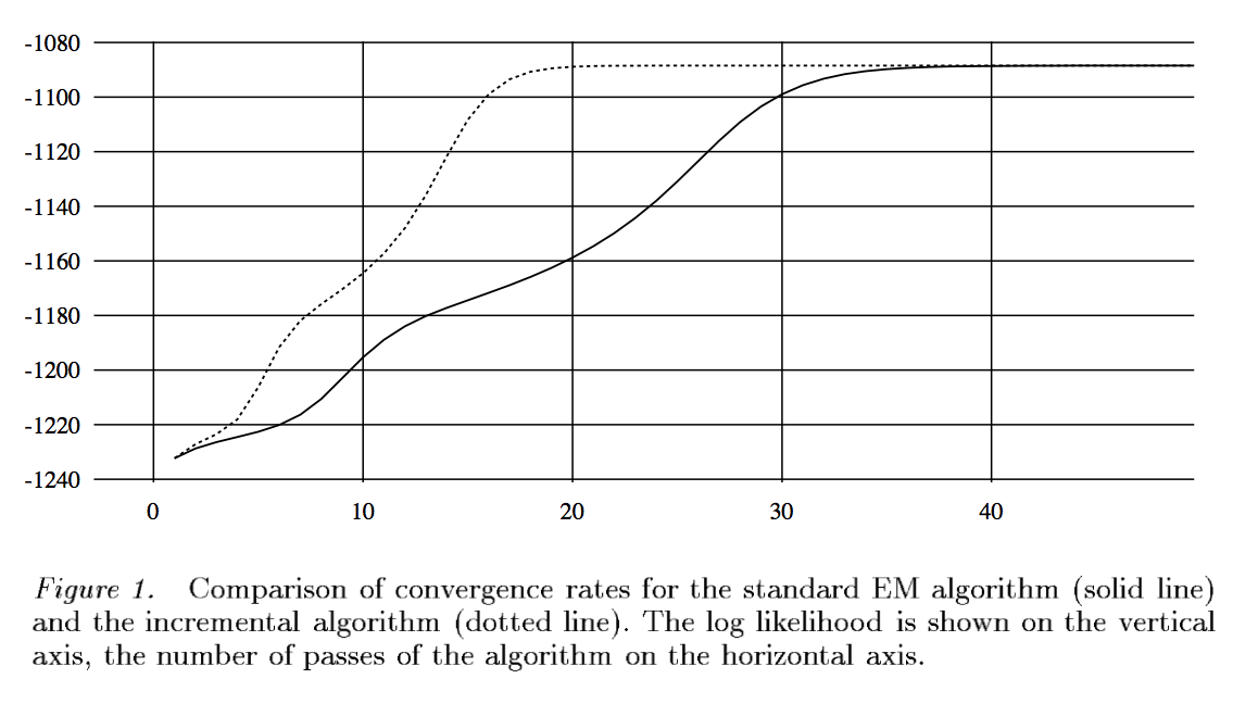
 ## Incremental EM
* Assume iid observations. Then the objective function is
\begin{eqnarray*}
F(\theta,q) = \sum_i \left[ \mathbf{E}_{q_i} \log p(\mathbf{Z}_i,\mathbf{y}_i \mid \theta) + H(q_i) \right],
\end{eqnarray*}
where we search for $q$ under factored form $q(\mathbf{z}) = \prod_i q_i (\mathbf{z})$.
* Maximizing $F$ over $q$ is equivalent to maximizing the contribution of each data with respect to $q_i$.
* Update $\theta$ by visiting data items **sequentially** rather than from a global E step.
* Finite mixture example: for each data point $i$
* evaluate membership variables $w_{ij}$, $j=1,\ldots,k$.
* update parameter values $(\pi^{(t+1)}, \mu_j^{(t+1)}, \Sigma_j^{(t+1)})$ (only need to keep sufficient statistics!)
* Faster convergence than vanilla EM in some examples.
## Incremental EM
* Assume iid observations. Then the objective function is
\begin{eqnarray*}
F(\theta,q) = \sum_i \left[ \mathbf{E}_{q_i} \log p(\mathbf{Z}_i,\mathbf{y}_i \mid \theta) + H(q_i) \right],
\end{eqnarray*}
where we search for $q$ under factored form $q(\mathbf{z}) = \prod_i q_i (\mathbf{z})$.
* Maximizing $F$ over $q$ is equivalent to maximizing the contribution of each data with respect to $q_i$.
* Update $\theta$ by visiting data items **sequentially** rather than from a global E step.
* Finite mixture example: for each data point $i$
* evaluate membership variables $w_{ij}$, $j=1,\ldots,k$.
* update parameter values $(\pi^{(t+1)}, \mu_j^{(t+1)}, \Sigma_j^{(t+1)})$ (only need to keep sufficient statistics!)
* Faster convergence than vanilla EM in some examples.