---
title: MM Algorithm (KL Chapter 12)
subtitle: Biostat/Biomath M257
author: Dr. Hua Zhou @ UCLA
date: today
format:
html:
theme: cosmo
embed-resources: true
number-sections: true
toc: true
toc-depth: 4
toc-location: left
code-fold: false
jupyter:
jupytext:
formats: 'ipynb,qmd'
text_representation:
extension: .qmd
format_name: quarto
format_version: '1.0'
jupytext_version: 1.14.5
kernelspec:
display_name: Julia 1.9.0
language: julia
name: julia-1.9
---

 ## MM algorithm
* Recall our picture for understanding the ascent property of EM
## MM algorithm
* Recall our picture for understanding the ascent property of EM
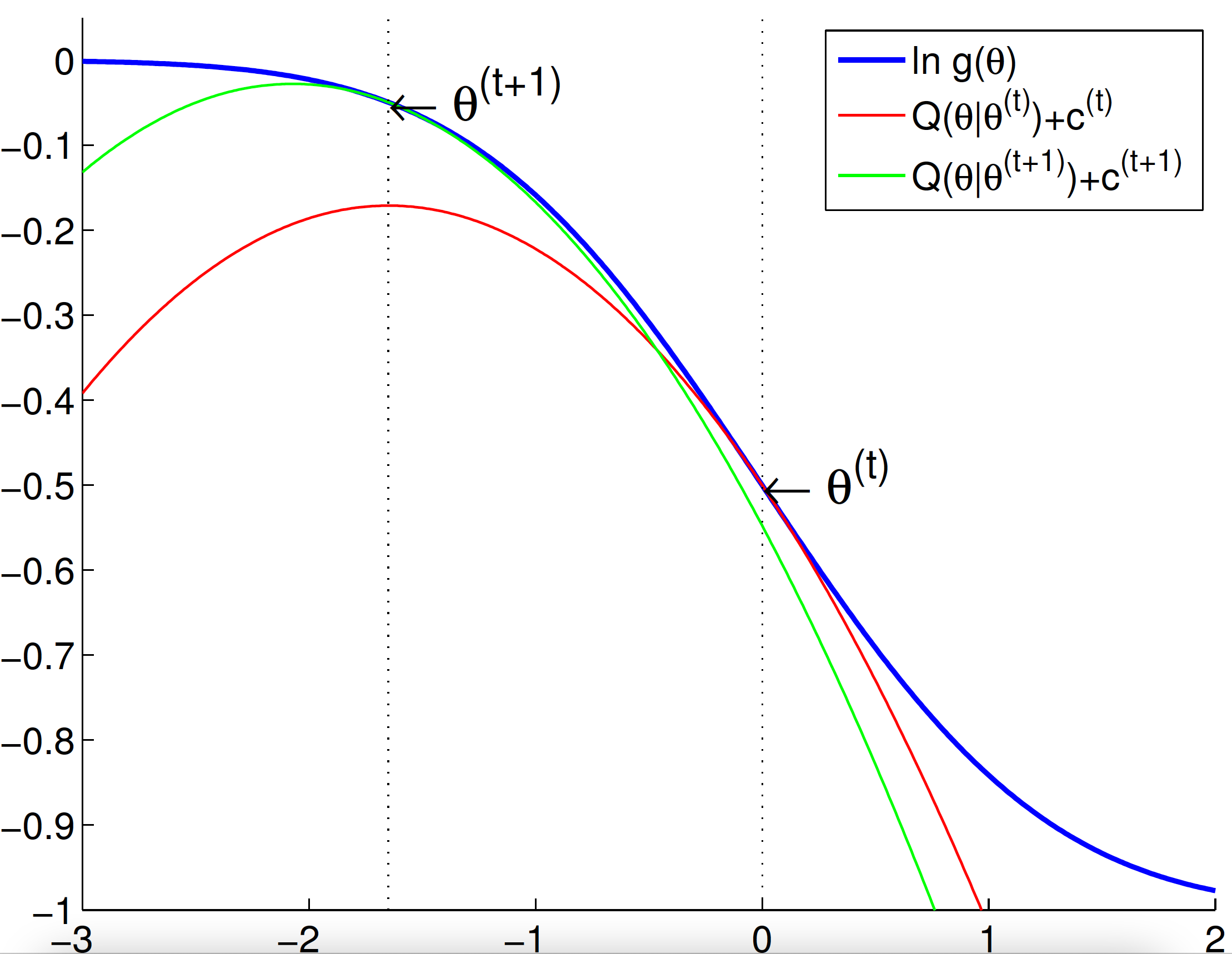
 * EM as a minorization-maximization (MM) algorithm
* The $Q$ function constitutes a **minorizing** function of the objective function up to an additive constant
$$
\begin{eqnarray*}
L(\theta) &\ge& Q(\theta|\theta^{(t)}) + c^{(t)} \quad \text{for all } \theta \\
L(\theta^{(t)}) &=& Q(\theta^{(t)}|\theta^{(t)}) + c^{(t)}
\end{eqnarray*}
$$
* **Maximizing** the $Q$ function generates an ascent iterate $\theta^{(t+1)}$
* Questions:
1. Is EM principle only limited to maximizing likelihood model?
2. Can we flip the picture and apply same principle to **minimization** problem?
3. Is there any other way to produce such surrogate function?
* These thoughts lead to a powerful tool - MM algorithm.
**Lange, K.**, Hunter, D. R., and Yang, I. (2000). Optimization transfer using surrogate objective functions. _J. Comput. Graph. Statist._, 9(1):1-59. With discussion, and a rejoinder by Hunter and Lange.
* For maximization of $f(\theta)$ - **minorization-maximization (MM)** algorithm
* **M**inorization step: Construct a surrogate function $g(\theta|\theta^{(t)})$ that satisfies
$$
\begin{eqnarray*}
f(\theta) &\ge& g(\theta|\theta^{(t)}) \quad \text{(dominance condition)} \\
f(\theta^{(t)}) &=& g(\theta^{(t)}|\theta^{(t)}) \quad \text{(tangent condition)}.
\end{eqnarray*}
$$
* **M**aximization step:
$$
\theta^{(t+1)} = \text{argmax} \, g(\theta|\theta^{(t)}).
$$
* _Ascent_ property of minorization-maximization algorithm
$$
f(\theta^{(t)}) = g(\theta^{(t)}|\theta^{(t)}) \le g(\theta^{(t+1)}|\theta^{(t)}) \le f(\theta^{(t+1)}).
$$
* EM is a special case of minorization-maximization (MM) algorithm.
* For minimization of $f(\theta)$ - **majorization-minimization (MM)** algorithm
* **M**ajorization step: Construct a surrogate function $g(\theta|\theta^{(t)})$ that satisfies
$$
\begin{eqnarray*}
f(\theta) &\le& g(\theta|\theta^{(t)}) \quad \text{(dominance condition)} \\
f(\theta^{(t)}) &=& g(\theta^{(t)}|\theta^{(t)}) \quad \text{(tangent condition)}.
\end{eqnarray*}
$$
* **M**inimization step:
$$
\theta^{(t+1)} = \text{argmin} \, g(\theta|\theta^{(t)}).
$$
* EM as a minorization-maximization (MM) algorithm
* The $Q$ function constitutes a **minorizing** function of the objective function up to an additive constant
$$
\begin{eqnarray*}
L(\theta) &\ge& Q(\theta|\theta^{(t)}) + c^{(t)} \quad \text{for all } \theta \\
L(\theta^{(t)}) &=& Q(\theta^{(t)}|\theta^{(t)}) + c^{(t)}
\end{eqnarray*}
$$
* **Maximizing** the $Q$ function generates an ascent iterate $\theta^{(t+1)}$
* Questions:
1. Is EM principle only limited to maximizing likelihood model?
2. Can we flip the picture and apply same principle to **minimization** problem?
3. Is there any other way to produce such surrogate function?
* These thoughts lead to a powerful tool - MM algorithm.
**Lange, K.**, Hunter, D. R., and Yang, I. (2000). Optimization transfer using surrogate objective functions. _J. Comput. Graph. Statist._, 9(1):1-59. With discussion, and a rejoinder by Hunter and Lange.
* For maximization of $f(\theta)$ - **minorization-maximization (MM)** algorithm
* **M**inorization step: Construct a surrogate function $g(\theta|\theta^{(t)})$ that satisfies
$$
\begin{eqnarray*}
f(\theta) &\ge& g(\theta|\theta^{(t)}) \quad \text{(dominance condition)} \\
f(\theta^{(t)}) &=& g(\theta^{(t)}|\theta^{(t)}) \quad \text{(tangent condition)}.
\end{eqnarray*}
$$
* **M**aximization step:
$$
\theta^{(t+1)} = \text{argmax} \, g(\theta|\theta^{(t)}).
$$
* _Ascent_ property of minorization-maximization algorithm
$$
f(\theta^{(t)}) = g(\theta^{(t)}|\theta^{(t)}) \le g(\theta^{(t+1)}|\theta^{(t)}) \le f(\theta^{(t+1)}).
$$
* EM is a special case of minorization-maximization (MM) algorithm.
* For minimization of $f(\theta)$ - **majorization-minimization (MM)** algorithm
* **M**ajorization step: Construct a surrogate function $g(\theta|\theta^{(t)})$ that satisfies
$$
\begin{eqnarray*}
f(\theta) &\le& g(\theta|\theta^{(t)}) \quad \text{(dominance condition)} \\
f(\theta^{(t)}) &=& g(\theta^{(t)}|\theta^{(t)}) \quad \text{(tangent condition)}.
\end{eqnarray*}
$$
* **M**inimization step:
$$
\theta^{(t+1)} = \text{argmin} \, g(\theta|\theta^{(t)}).
$$
 * Similarly we have the _descent_ property of majorization-minimization algorithm.
* Same convergence theory as EM.
* Rational of the MM principle for developing optimization algorithms
* Free the derivation from missing data structure.
* Avoid matrix inversion.
* Linearize an optimization problem.
* Deal gracefully with certain equality and inequality constraints.
* Turn a non-differentiable problem into a smooth problem.
* Separate the parameters of a problem (perfect for massive, _fine-scale_ parallelization).
* Generic methods for majorization and minorization - **inequalities**
* Jensen's (information) inequality - EM algorithms
* Supporting hyperplane property of a convex function
* The Cauchy-Schwarz inequality - multidimensional scaling
* Arithmetic-geometric mean inequality
* Quadratic upper bound principle - Bohning and Lindsay
* ...
* Numerous examples in KL chapter 12, or take Kenneth Lange's optimization course BIOMATH 210.
* History: the name _MM algorithm_ originates from the discussion (by Xiaoli Meng) and rejoinder of the Lange, Hunter, Yang (2000) paper.
## MM example: t-distribution revisited
* Recall that given iid data $\mathbf{w}_1, \ldots, \mathbf{w}_n$ from multivariate $t$-distribution $t_p(\mu,\Sigma,\nu)$, the log-likelihood is
\begin{eqnarray*}
L(\mu, \Sigma, \nu) &=& - \frac{np}{2} \log (\pi \nu) + n \left[ \log \Gamma \left(\frac{\nu+p}{2}\right) - \log \Gamma \left(\frac{\nu}{2}\right) \right] \\
&& - \frac n2 \log \det \Sigma + \frac n2 (\nu + p) \log \nu \\
&& - \frac{\nu + p}{2} \sum_{j=1}^n \log [\nu + \delta (\mathbf{w}_j,\mu;\Sigma) ].
\end{eqnarray*}
* Early on we discussed EM algorithm and its variants for maximizing the log-likelihood.
* Since $t \mapsto - \log t$ is a convex function, we can invoke the supporting hyperplane inequality to minorize the terms $- \log [\nu + \delta (\mathbf{w}_j,\mu;\Sigma)$:
\begin{eqnarray*}
\, - \log [\nu + \delta (\mathbf{w}_j,\mu;\Sigma)] &\ge& - \log [\nu^{(t)} + \delta (\mathbf{w}_j,\mu^{(t)};\Sigma^{(t)})] - \frac{\nu + \delta (\mathbf{w}_j,\mu;\Sigma) - \nu^{(t)} - \delta (\mathbf{w}_j,\mu^{(t)};\Sigma^{(t)})}{\nu^{(t)} + \delta (\mathbf{w}_j,\mu^{(t)};\Sigma^{(t)})} \\
&=& - \frac{\nu + \delta (\mathbf{w}_j,\mu;\Sigma)}{\nu^{(t)} + \delta (\mathbf{w}_j,\mu^{(t)};\Sigma^{(t)})} + c^{(t)},
\end{eqnarray*}
where $c^{(t)}$ is a constant irrelevant to optimization.
* This yields a minorization function
\begin{eqnarray*}
g(\mu, \Sigma, \nu) &=& - \frac{np}{2} \log (\pi \nu) + n \left[ \log \Gamma \left(\frac{\nu+p}{2}\right) - \log \Gamma \left(\frac{\nu}{2}\right) \right] \\
&& - \frac n2 \log \det \Sigma + \frac n2 (\nu + p) \log \nu \\
&& - \frac{\nu + p}{2} \sum_{j=1}^n \frac{\nu + \delta (\mathbf{w}_j,\mu;\Sigma)}{\nu^{(t)} + \delta (\mathbf{w}_j,\mu^{(t)};\Sigma^{(t)})} + c^{(t)}.
\end{eqnarray*}
Now we can deploy the block ascent strategy.
* Fixing $\nu$, update of $\mu$ and $\Sigma$ are same as in EM algorithm.
* Fixing $\mu$ and $\Sigma$, we can update $\nu$ by working on the observed log-likelihood directly.
Overall this MM algorithm coincides with ECME.
* An alternative MM derivation leads to the optimal EM algorithm derived in Meng and van Dyk (1997). See [Wu and Lange (2010)](https://doi.org/10.1214/08-STS264).
## MM example: non-negative matrix factorization (NNMF)
* Similarly we have the _descent_ property of majorization-minimization algorithm.
* Same convergence theory as EM.
* Rational of the MM principle for developing optimization algorithms
* Free the derivation from missing data structure.
* Avoid matrix inversion.
* Linearize an optimization problem.
* Deal gracefully with certain equality and inequality constraints.
* Turn a non-differentiable problem into a smooth problem.
* Separate the parameters of a problem (perfect for massive, _fine-scale_ parallelization).
* Generic methods for majorization and minorization - **inequalities**
* Jensen's (information) inequality - EM algorithms
* Supporting hyperplane property of a convex function
* The Cauchy-Schwarz inequality - multidimensional scaling
* Arithmetic-geometric mean inequality
* Quadratic upper bound principle - Bohning and Lindsay
* ...
* Numerous examples in KL chapter 12, or take Kenneth Lange's optimization course BIOMATH 210.
* History: the name _MM algorithm_ originates from the discussion (by Xiaoli Meng) and rejoinder of the Lange, Hunter, Yang (2000) paper.
## MM example: t-distribution revisited
* Recall that given iid data $\mathbf{w}_1, \ldots, \mathbf{w}_n$ from multivariate $t$-distribution $t_p(\mu,\Sigma,\nu)$, the log-likelihood is
\begin{eqnarray*}
L(\mu, \Sigma, \nu) &=& - \frac{np}{2} \log (\pi \nu) + n \left[ \log \Gamma \left(\frac{\nu+p}{2}\right) - \log \Gamma \left(\frac{\nu}{2}\right) \right] \\
&& - \frac n2 \log \det \Sigma + \frac n2 (\nu + p) \log \nu \\
&& - \frac{\nu + p}{2} \sum_{j=1}^n \log [\nu + \delta (\mathbf{w}_j,\mu;\Sigma) ].
\end{eqnarray*}
* Early on we discussed EM algorithm and its variants for maximizing the log-likelihood.
* Since $t \mapsto - \log t$ is a convex function, we can invoke the supporting hyperplane inequality to minorize the terms $- \log [\nu + \delta (\mathbf{w}_j,\mu;\Sigma)$:
\begin{eqnarray*}
\, - \log [\nu + \delta (\mathbf{w}_j,\mu;\Sigma)] &\ge& - \log [\nu^{(t)} + \delta (\mathbf{w}_j,\mu^{(t)};\Sigma^{(t)})] - \frac{\nu + \delta (\mathbf{w}_j,\mu;\Sigma) - \nu^{(t)} - \delta (\mathbf{w}_j,\mu^{(t)};\Sigma^{(t)})}{\nu^{(t)} + \delta (\mathbf{w}_j,\mu^{(t)};\Sigma^{(t)})} \\
&=& - \frac{\nu + \delta (\mathbf{w}_j,\mu;\Sigma)}{\nu^{(t)} + \delta (\mathbf{w}_j,\mu^{(t)};\Sigma^{(t)})} + c^{(t)},
\end{eqnarray*}
where $c^{(t)}$ is a constant irrelevant to optimization.
* This yields a minorization function
\begin{eqnarray*}
g(\mu, \Sigma, \nu) &=& - \frac{np}{2} \log (\pi \nu) + n \left[ \log \Gamma \left(\frac{\nu+p}{2}\right) - \log \Gamma \left(\frac{\nu}{2}\right) \right] \\
&& - \frac n2 \log \det \Sigma + \frac n2 (\nu + p) \log \nu \\
&& - \frac{\nu + p}{2} \sum_{j=1}^n \frac{\nu + \delta (\mathbf{w}_j,\mu;\Sigma)}{\nu^{(t)} + \delta (\mathbf{w}_j,\mu^{(t)};\Sigma^{(t)})} + c^{(t)}.
\end{eqnarray*}
Now we can deploy the block ascent strategy.
* Fixing $\nu$, update of $\mu$ and $\Sigma$ are same as in EM algorithm.
* Fixing $\mu$ and $\Sigma$, we can update $\nu$ by working on the observed log-likelihood directly.
Overall this MM algorithm coincides with ECME.
* An alternative MM derivation leads to the optimal EM algorithm derived in Meng and van Dyk (1997). See [Wu and Lange (2010)](https://doi.org/10.1214/08-STS264).
## MM example: non-negative matrix factorization (NNMF)
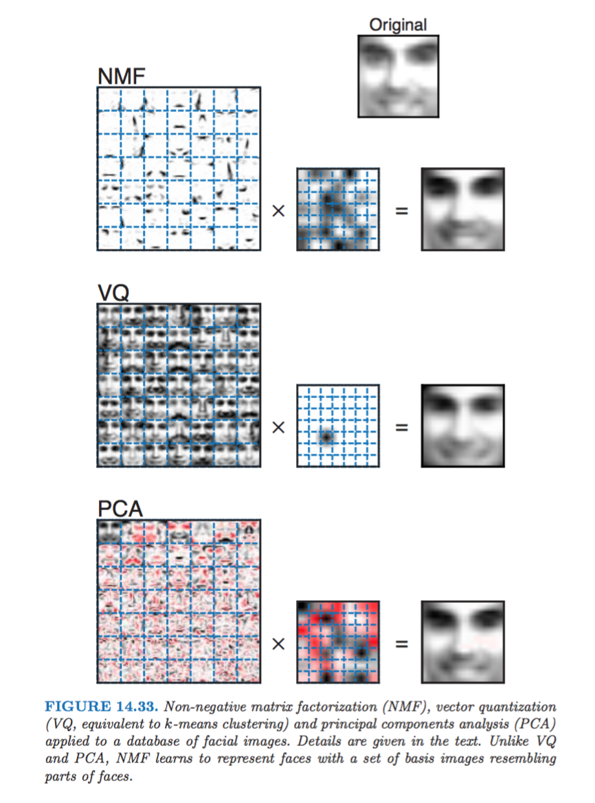 * Nonnegative matrix factorization (NNMF) was introduced by Lee and Seung ([1999](http://www.nature.com/nature/journal/v401/n6755/abs/401788a0.html), [2001](https://papers.nips.cc/paper/1861-algorithms-for-non-negative-matrix-factorization.pdf)) as an analog of principal components and vector quantization with applications in data compression and clustering.
* In mathematical terms, one approximates a data matrix $\mathbf{X} \in \mathbb{R}^{m \times n}$ with nonnegative entries $x_{ij}$ by a product of two low-rank matrices $\mathbf{V} \in \mathbb{R}^{m \times r}$ and $\mathbf{W} \in \mathbb{R}^{r \times n}$ with nonnegative entries $v_{ik}$ and $w_{kj}$.
* Consider minimization of the squared Frobenius norm
$$
L(\mathbf{V}, \mathbf{W}) = \|\mathbf{X} - \mathbf{V} \mathbf{W}\|_{\text{F}}^2 = \sum_i \sum_j \left( x_{ij} - \sum_k v_{ik} w_{kj} \right)^2, \quad v_{ik} \ge 0, w_{kj} \ge 0,
$$
which should lead to a good factorization.
* $L(\mathbf{V}, \mathbf{W})$ is not convex, but bi-convex. The strategy is to alternately update $\mathbf{V}$ and $\mathbf{W}$.
* The key is the majorization, via convexity of the function $(x_{ij} - x)^2$,
$$
\left( x_{ij} - \sum_k v_{ik} w_{kj} \right)^2 \le \sum_k \frac{a_{ikj}^{(t)}}{b_{ij}^{(t)}} \left( x_{ij} - \frac{b_{ij}^{(t)}}{a_{ikj}^{(t)}} v_{ik} w_{kj} \right)^2,
$$
where
$$
a_{ikj}^{(t)} = v_{ik}^{(t)} w_{kj}^{(t)}, \quad b_{ij}^{(t)} = \sum_k v_{ik}^{(t)} w_{kj}^{(t)}.
$$
* This suggests the alternating multiplicative updates
$$
\begin{eqnarray*}
v_{ik}^{(t+1)} &=& v_{ik}^{(t)} \frac{\sum_j x_{ij} w_{kj}^{(t)}}{\sum_j b_{ij}^{(t)} w_{kj}^{(t)}} \\
b_{ij}^{(t+1/2)} &=& \sum_k v_{ik}^{(t+1)} w_{kj}^{(t)} \\
w_{kj}^{(t+1)} &=& w_{kj}^{(t)} \frac{\sum_i x_{ij} v_{ik}^{(t+1)}}{\sum_i b_{ij}^{(t+1/2)} v_{ik}^{(t+1)}}.
\end{eqnarray*}
$$
* The update in matrix notation is extremely simple
$$
\begin{eqnarray*}
\mathbf{B}^{(t)} &=& \mathbf{V}^{(t)} \mathbf{W}^{(t)} \\
\mathbf{V}^{(t+1)} &=& \mathbf{V}^{(t)} \odot (\mathbf{X} \mathbf{W}^{(t)T}) \oslash (\mathbf{B}^{(t)} \mathbf{W}^{(t)T}) \\
\mathbf{B}^{(t+1/2)} &=& \mathbf{V}^{(t+1)} \mathbf{W}^{(t)} \\
\mathbf{W}^{(t+1)} &=& \mathbf{W}^{(t)} \odot (\mathbf{X}^T \mathbf{V}^{(t+1)}) \oslash (\mathbf{B}^{(t+1/2)T} \mathbf{V}^{(t)}),
\end{eqnarray*}
$$
where $\odot$ denotes elementwise multiplication and $\oslash$ denotes elementwise division. If we start with $v_{ik}, w_{kj} > 0$, parameter iterates stay positive.
* Monotoniciy of the algorithm is free (from MM principle).
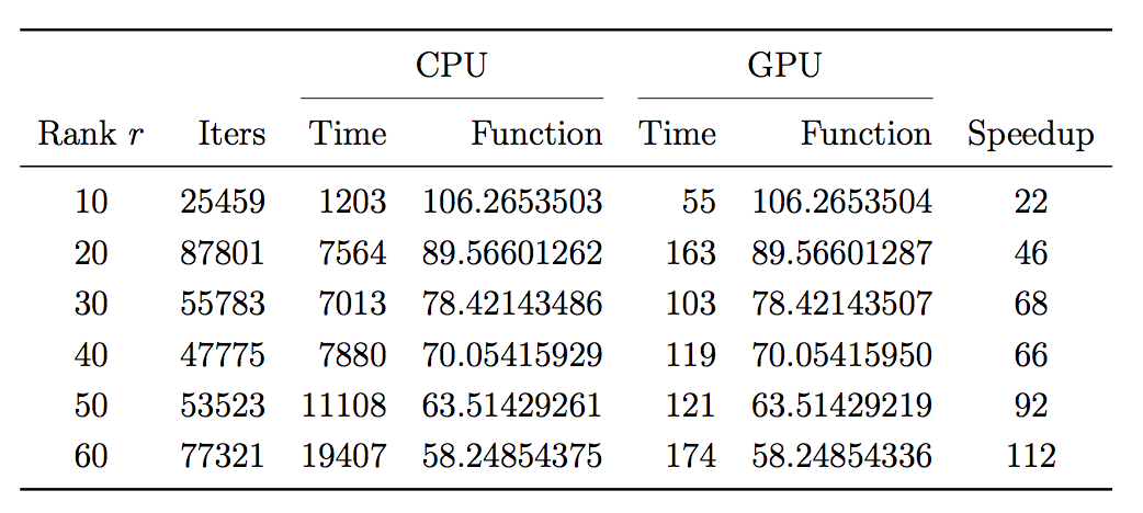
* Database \#1 from the MIT Center for Biological and Computational Learning (CBCL, http://cbcl.mit.edu) reduces to a matrix X containing $m = 2,429$ gray-scale face images with $n = 19 \times 19 = 361$ pixels per face. Each image (row) is scaled to have mean and standard deviation 0.25.
* My implementation in around **2010**:
CPU: Intel Core 2 @ 3.2GHZ (4 cores), implemented using BLAS in the GNU Scientific Library (GSL)
GPU: NVIDIA GeForce GTX 280 (240 cores), implemented using cuBLAS.
* Nonnegative matrix factorization (NNMF) was introduced by Lee and Seung ([1999](http://www.nature.com/nature/journal/v401/n6755/abs/401788a0.html), [2001](https://papers.nips.cc/paper/1861-algorithms-for-non-negative-matrix-factorization.pdf)) as an analog of principal components and vector quantization with applications in data compression and clustering.
* In mathematical terms, one approximates a data matrix $\mathbf{X} \in \mathbb{R}^{m \times n}$ with nonnegative entries $x_{ij}$ by a product of two low-rank matrices $\mathbf{V} \in \mathbb{R}^{m \times r}$ and $\mathbf{W} \in \mathbb{R}^{r \times n}$ with nonnegative entries $v_{ik}$ and $w_{kj}$.
* Consider minimization of the squared Frobenius norm
$$
L(\mathbf{V}, \mathbf{W}) = \|\mathbf{X} - \mathbf{V} \mathbf{W}\|_{\text{F}}^2 = \sum_i \sum_j \left( x_{ij} - \sum_k v_{ik} w_{kj} \right)^2, \quad v_{ik} \ge 0, w_{kj} \ge 0,
$$
which should lead to a good factorization.
* $L(\mathbf{V}, \mathbf{W})$ is not convex, but bi-convex. The strategy is to alternately update $\mathbf{V}$ and $\mathbf{W}$.
* The key is the majorization, via convexity of the function $(x_{ij} - x)^2$,
$$
\left( x_{ij} - \sum_k v_{ik} w_{kj} \right)^2 \le \sum_k \frac{a_{ikj}^{(t)}}{b_{ij}^{(t)}} \left( x_{ij} - \frac{b_{ij}^{(t)}}{a_{ikj}^{(t)}} v_{ik} w_{kj} \right)^2,
$$
where
$$
a_{ikj}^{(t)} = v_{ik}^{(t)} w_{kj}^{(t)}, \quad b_{ij}^{(t)} = \sum_k v_{ik}^{(t)} w_{kj}^{(t)}.
$$
* This suggests the alternating multiplicative updates
$$
\begin{eqnarray*}
v_{ik}^{(t+1)} &=& v_{ik}^{(t)} \frac{\sum_j x_{ij} w_{kj}^{(t)}}{\sum_j b_{ij}^{(t)} w_{kj}^{(t)}} \\
b_{ij}^{(t+1/2)} &=& \sum_k v_{ik}^{(t+1)} w_{kj}^{(t)} \\
w_{kj}^{(t+1)} &=& w_{kj}^{(t)} \frac{\sum_i x_{ij} v_{ik}^{(t+1)}}{\sum_i b_{ij}^{(t+1/2)} v_{ik}^{(t+1)}}.
\end{eqnarray*}
$$
* The update in matrix notation is extremely simple
$$
\begin{eqnarray*}
\mathbf{B}^{(t)} &=& \mathbf{V}^{(t)} \mathbf{W}^{(t)} \\
\mathbf{V}^{(t+1)} &=& \mathbf{V}^{(t)} \odot (\mathbf{X} \mathbf{W}^{(t)T}) \oslash (\mathbf{B}^{(t)} \mathbf{W}^{(t)T}) \\
\mathbf{B}^{(t+1/2)} &=& \mathbf{V}^{(t+1)} \mathbf{W}^{(t)} \\
\mathbf{W}^{(t+1)} &=& \mathbf{W}^{(t)} \odot (\mathbf{X}^T \mathbf{V}^{(t+1)}) \oslash (\mathbf{B}^{(t+1/2)T} \mathbf{V}^{(t)}),
\end{eqnarray*}
$$
where $\odot$ denotes elementwise multiplication and $\oslash$ denotes elementwise division. If we start with $v_{ik}, w_{kj} > 0$, parameter iterates stay positive.
* Monotoniciy of the algorithm is free (from MM principle).
* Database \#1 from the MIT Center for Biological and Computational Learning (CBCL, http://cbcl.mit.edu) reduces to a matrix X containing $m = 2,429$ gray-scale face images with $n = 19 \times 19 = 361$ pixels per face. Each image (row) is scaled to have mean and standard deviation 0.25.
* My implementation in around **2010**:
CPU: Intel Core 2 @ 3.2GHZ (4 cores), implemented using BLAS in the GNU Scientific Library (GSL)
GPU: NVIDIA GeForce GTX 280 (240 cores), implemented using cuBLAS.
 ## MM example: Netflix and matrix completion
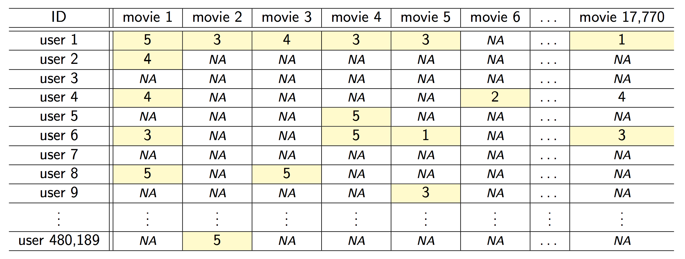
* Snapshot of the kind of data collected by Netflix. Only 100,480,507 ratings (1.2% entries of the 480K-by-18K matrix) are observed
## MM example: Netflix and matrix completion
* Snapshot of the kind of data collected by Netflix. Only 100,480,507 ratings (1.2% entries of the 480K-by-18K matrix) are observed
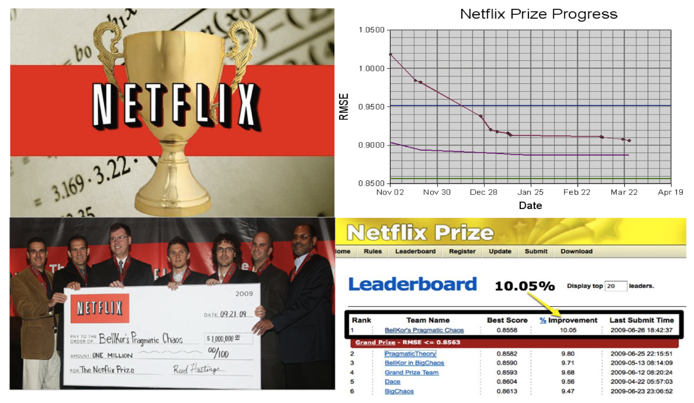
 * Netflix challenge: impute the unobserved ratings for personalized recommendation.
http://en.wikipedia.org/wiki/Netflix_Prize
* Netflix challenge: impute the unobserved ratings for personalized recommendation.
http://en.wikipedia.org/wiki/Netflix_Prize
 * **Matrix completion problem**. Observe a very sparse matrix $\mathbf{Y} = (y_{ij})$. Want to impute all the missing entries. It is possible only when the matrix is structured, e.g., of _low rank_.
* Let $\Omega = \{(i,j): \text{observed entries}\}$ index the set of observed entries and $P_\Omega(\mathbf{M})$ denote the projection of matrix $\mathbf{M}$ to $\Omega$. The problem
$$
\min_{\text{rank}(\mathbf{X}) \le r} \frac{1}{2} \| P_\Omega(\mathbf{Y}) - P_\Omega(\mathbf{X})\|_{\text{F}}^2 = \frac{1}{2} \sum_{(i,j) \in \Omega} (y_{ij} - x_{ij})^2
$$
unfortunately is non-convex and difficult.
* _Convex relaxation_: [Mazumder, Hastie, Tibshirani (2010)](https://web.stanford.edu/~hastie/Papers/mazumder10a.pdf)
$$
\min_{\mathbf{X}} f(\mathbf{X}) = \frac{1}{2} \| P_\Omega(\mathbf{Y}) - P_\Omega(\mathbf{X})\|_{\text{F}}^2 + \lambda \|\mathbf{X}\|_*,
$$
where $\|\mathbf{X}\|_* = \|\sigma(\mathbf{X})\|_1 = \sum_i \sigma_i(\mathbf{X})$ is the nuclear norm.
* **Majorization step**:
$$
\begin{eqnarray*}
f(\mathbf{X}) &=& \frac{1}{2} \sum_{(i,j) \in \Omega} (y_{ij} - x_{ij})^2 + \frac 12 \sum_{(i,j) \notin \Omega} 0 + \lambda \|\mathbf{X}\|_* \\
&\le& \frac{1}{2} \sum_{(i,j) \in \Omega} (y_{ij} - x_{ij})^2 + \frac{1}{2} \sum_{(i,j) \notin \Omega} (x_{ij}^{(t)} - x_{ij})^2 + \lambda \|\mathbf{X}\|_* \\
&=& \frac{1}{2} \| \mathbf{X} - \mathbf{Z}^{(t)}\|_{\text{F}}^2 + \lambda \|\mathbf{X}\|_* \\
&=& g(\mathbf{X}|\mathbf{X}^{(t)}),
\end{eqnarray*}
$$
where $\mathbf{Z}^{(t)} = P_\Omega(\mathbf{Y}) + P_{\Omega^\perp}(\mathbf{X}^{(t)})$. "fill in missing entries by the current imputation"
* **Minimization step**: Rewrite the surrogate function
$$
\begin{eqnarray*}
g(\mathbf{X}|\mathbf{X}^{(t)}) = \frac{1}{2} \|\mathbf{X}\|_{\text{F}}^2 - \text{tr}(\mathbf{X}^T \mathbf{Z}^{(t)}) + \frac{1}{2} \|\mathbf{Z}^{(t)}\|_{\text{F}}^2 + \lambda \|\mathbf{X}\|_*.
\end{eqnarray*}
$$
Let $\sigma_i$ be the (ordered) singular values of $\mathbf{X}$ and $\omega_i$ be the (ordered) singular values of $\mathbf{Z}^{(t)}$. Observe
$$
\begin{eqnarray*}
\|\mathbf{X}\|_{\text{F}}^2 &=& \|\sigma(\mathbf{X})\|_2^2 = \sum_{i} \sigma_i^2 \\
\|\mathbf{Z}^{(t)}\|_{\text{F}}^2 &=& \|\sigma(\mathbf{Z}^{(t)})\|_2^2 = \sum_{i} \omega_i^2
\end{eqnarray*}
$$
and by the [Fan-von Neuman's inequality](https://en.wikipedia.org/wiki/Trace_inequalities#Von_Neumann.27s_trace_inequality)
$$
\begin{eqnarray*}
\text{tr}(\mathbf{X}^T \mathbf{Z}^{(t)}) \le \sum_i \sigma_i \omega_i
\end{eqnarray*}
$$
with equality achieved if and only if the left and right singular vectors of the two matrices coincide. Thus we should choose $\mathbf{X}$ to have same singular vectors as $\mathbf{Z}^{(t)}$ and
$$
\begin{eqnarray*}
g(\mathbf{X}|\mathbf{X}^{(t)}) &=& \frac{1}{2} \sum_i \sigma_i^2 - \sum_i \sigma_i \omega_i + \frac{1}{2} \sum_i \omega_i^2 + \lambda \sum_i \sigma_i \\
&=& \frac{1}{2} \sum_i (\sigma_i - \omega_i)^2 + \lambda \sum_i \sigma_i,
\end{eqnarray*}
$$
with minimizer given by **singular value thresholding**
$$
\sigma_i^{(t+1)} = \max(0, \omega_i - \lambda) = (\omega_i - \lambda)_+.
$$
* Algorithm for matrix completion:
* Initialize $\mathbf{X}^{(0)} \in \mathbb{R}^{m \times n}$
* Repeat
* $\mathbf{Z}^{(t)} \gets P_\Omega(\mathbf{Y}) + P_{\Omega^\perp}(\mathbf{X}^{(t)})$
* Compute SVD: $\mathbf{U} \text{diag}(\mathbf{w}) \mathbf{V}^T \gets \mathbf{Z}^{(t)}$
* $\mathbf{X}^{(t+1)} \gets \mathbf{U} \text{diag}[(\mathbf{w}-\lambda)_+] \mathbf{V}^T$
* objective value converges
* "Golub-Kahan-Reinsch" algorithm takes $4m^2n + 8mn^2 + 9n^3$ flops for an $m \ge n$ matrix and is **not** going to work for 480K-by-18K Netflix matrix.
* Notice only top singular values are needed since low rank solutions are achieved by large $\lambda$. Lanczos/Arnoldi algorithm is the way to go. Matrix-vector multiplication $\mathbf{Z}^{(t)} \mathbf{v}$ is fast (why?)
* **Matrix completion problem**. Observe a very sparse matrix $\mathbf{Y} = (y_{ij})$. Want to impute all the missing entries. It is possible only when the matrix is structured, e.g., of _low rank_.
* Let $\Omega = \{(i,j): \text{observed entries}\}$ index the set of observed entries and $P_\Omega(\mathbf{M})$ denote the projection of matrix $\mathbf{M}$ to $\Omega$. The problem
$$
\min_{\text{rank}(\mathbf{X}) \le r} \frac{1}{2} \| P_\Omega(\mathbf{Y}) - P_\Omega(\mathbf{X})\|_{\text{F}}^2 = \frac{1}{2} \sum_{(i,j) \in \Omega} (y_{ij} - x_{ij})^2
$$
unfortunately is non-convex and difficult.
* _Convex relaxation_: [Mazumder, Hastie, Tibshirani (2010)](https://web.stanford.edu/~hastie/Papers/mazumder10a.pdf)
$$
\min_{\mathbf{X}} f(\mathbf{X}) = \frac{1}{2} \| P_\Omega(\mathbf{Y}) - P_\Omega(\mathbf{X})\|_{\text{F}}^2 + \lambda \|\mathbf{X}\|_*,
$$
where $\|\mathbf{X}\|_* = \|\sigma(\mathbf{X})\|_1 = \sum_i \sigma_i(\mathbf{X})$ is the nuclear norm.
* **Majorization step**:
$$
\begin{eqnarray*}
f(\mathbf{X}) &=& \frac{1}{2} \sum_{(i,j) \in \Omega} (y_{ij} - x_{ij})^2 + \frac 12 \sum_{(i,j) \notin \Omega} 0 + \lambda \|\mathbf{X}\|_* \\
&\le& \frac{1}{2} \sum_{(i,j) \in \Omega} (y_{ij} - x_{ij})^2 + \frac{1}{2} \sum_{(i,j) \notin \Omega} (x_{ij}^{(t)} - x_{ij})^2 + \lambda \|\mathbf{X}\|_* \\
&=& \frac{1}{2} \| \mathbf{X} - \mathbf{Z}^{(t)}\|_{\text{F}}^2 + \lambda \|\mathbf{X}\|_* \\
&=& g(\mathbf{X}|\mathbf{X}^{(t)}),
\end{eqnarray*}
$$
where $\mathbf{Z}^{(t)} = P_\Omega(\mathbf{Y}) + P_{\Omega^\perp}(\mathbf{X}^{(t)})$. "fill in missing entries by the current imputation"
* **Minimization step**: Rewrite the surrogate function
$$
\begin{eqnarray*}
g(\mathbf{X}|\mathbf{X}^{(t)}) = \frac{1}{2} \|\mathbf{X}\|_{\text{F}}^2 - \text{tr}(\mathbf{X}^T \mathbf{Z}^{(t)}) + \frac{1}{2} \|\mathbf{Z}^{(t)}\|_{\text{F}}^2 + \lambda \|\mathbf{X}\|_*.
\end{eqnarray*}
$$
Let $\sigma_i$ be the (ordered) singular values of $\mathbf{X}$ and $\omega_i$ be the (ordered) singular values of $\mathbf{Z}^{(t)}$. Observe
$$
\begin{eqnarray*}
\|\mathbf{X}\|_{\text{F}}^2 &=& \|\sigma(\mathbf{X})\|_2^2 = \sum_{i} \sigma_i^2 \\
\|\mathbf{Z}^{(t)}\|_{\text{F}}^2 &=& \|\sigma(\mathbf{Z}^{(t)})\|_2^2 = \sum_{i} \omega_i^2
\end{eqnarray*}
$$
and by the [Fan-von Neuman's inequality](https://en.wikipedia.org/wiki/Trace_inequalities#Von_Neumann.27s_trace_inequality)
$$
\begin{eqnarray*}
\text{tr}(\mathbf{X}^T \mathbf{Z}^{(t)}) \le \sum_i \sigma_i \omega_i
\end{eqnarray*}
$$
with equality achieved if and only if the left and right singular vectors of the two matrices coincide. Thus we should choose $\mathbf{X}$ to have same singular vectors as $\mathbf{Z}^{(t)}$ and
$$
\begin{eqnarray*}
g(\mathbf{X}|\mathbf{X}^{(t)}) &=& \frac{1}{2} \sum_i \sigma_i^2 - \sum_i \sigma_i \omega_i + \frac{1}{2} \sum_i \omega_i^2 + \lambda \sum_i \sigma_i \\
&=& \frac{1}{2} \sum_i (\sigma_i - \omega_i)^2 + \lambda \sum_i \sigma_i,
\end{eqnarray*}
$$
with minimizer given by **singular value thresholding**
$$
\sigma_i^{(t+1)} = \max(0, \omega_i - \lambda) = (\omega_i - \lambda)_+.
$$
* Algorithm for matrix completion:
* Initialize $\mathbf{X}^{(0)} \in \mathbb{R}^{m \times n}$
* Repeat
* $\mathbf{Z}^{(t)} \gets P_\Omega(\mathbf{Y}) + P_{\Omega^\perp}(\mathbf{X}^{(t)})$
* Compute SVD: $\mathbf{U} \text{diag}(\mathbf{w}) \mathbf{V}^T \gets \mathbf{Z}^{(t)}$
* $\mathbf{X}^{(t+1)} \gets \mathbf{U} \text{diag}[(\mathbf{w}-\lambda)_+] \mathbf{V}^T$
* objective value converges
* "Golub-Kahan-Reinsch" algorithm takes $4m^2n + 8mn^2 + 9n^3$ flops for an $m \ge n$ matrix and is **not** going to work for 480K-by-18K Netflix matrix.
* Notice only top singular values are needed since low rank solutions are achieved by large $\lambda$. Lanczos/Arnoldi algorithm is the way to go. Matrix-vector multiplication $\mathbf{Z}^{(t)} \mathbf{v}$ is fast (why?)