---
title: 'Convexity, Duality, and Optimality Conditions (KL Chapter 11, BV Chapter 5)'
subtitle: Biostat/Biomath M257
author: Dr. Hua Zhou @ UCLA
date: today
format:
html:
theme: cosmo
embed-resources: true
number-sections: true
toc: true
toc-depth: 4
toc-location: left
code-fold: false
jupyter:
jupytext:
formats: 'ipynb,qmd'
text_representation:
extension: .qmd
format_name: quarto
format_version: '1.0'
jupytext_version: 1.14.5
kernelspec:
display_name: Julia 1.9.0
language: julia
name: julia-1.9
---
## Convexity
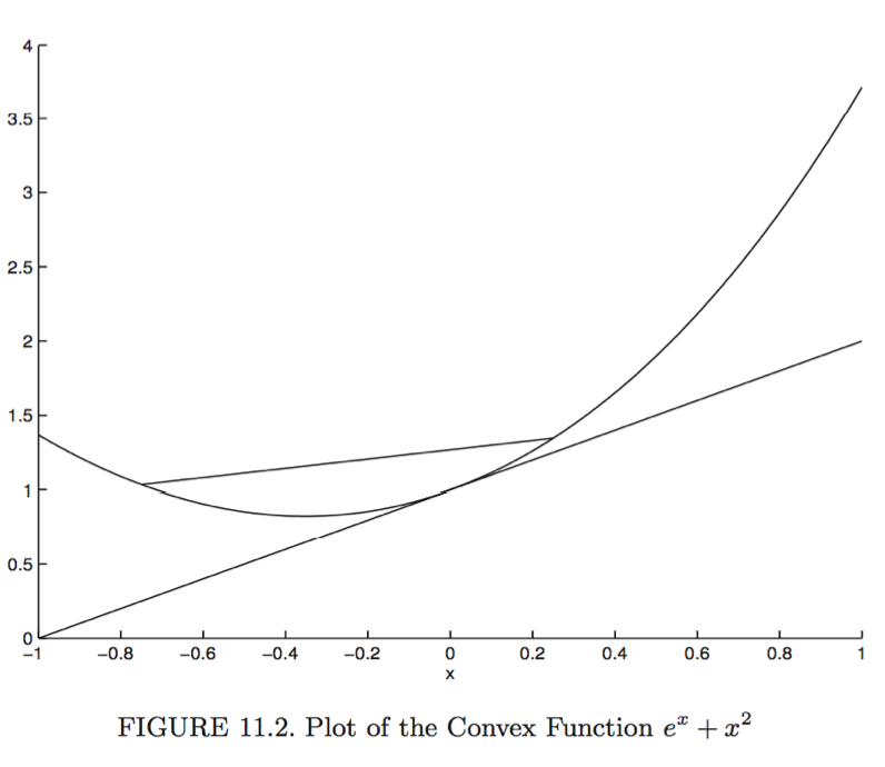 * A function $f: \mathbb{R}^n \mapsto \mathbb{R}$ is **convex** if
1. $\text{dom} f$ is a convex set: $\lambda \mathbf{x} + (1-\lambda) \mathbf{y} \in \text{dom} f$ for all $\mathbf{x},\mathbf{y} \in \text{dom} f$ and any $\lambda \in (0, 1)$, and
2. $f(\lambda \mathbf{x} + (1-\lambda) \mathbf{y}) \le \lambda f(\mathbf{x}) + (1-\lambda) f(\mathbf{y})$, for all $\mathbf{x},\mathbf{y} \in \text{dom} f$ and $\lambda \in (0,1)$.
* $f$ is **strictly convex** if the inequality is strict for all $\mathbf{x} \ne \mathbf{y} \in \text{dom} f$ and $\lambda$.
* **Supporting hyperplane inequality**. A differentiable function $f$ is convex if and only if
$$
f(\mathbf{x}) \ge f(\mathbf{y}) + \nabla f(\mathbf{y})^T (\mathbf{x}-\mathbf{y})
$$
for all $\mathbf{x}, \mathbf{y} \in \text{dom} f$.
Proof: For the only if part.
$$
f[\lambda x + (1 - \lambda) y)] \le \lambda f(x) + (1 - \lambda) f(y).
$$
Thus
$$
\frac{f(y + \lambda (x - y)) - f(y)}{\lambda} \le f(x) - f(y).
$$
Taking limit $\lambda \to 0$ yields the supporting hyperplane inequality. For the if part, let $z = \lambda x + (1 - \lambda) y$. Then
\begin{eqnarray*}
f(x) - f(z) &\ge& f'(z) (x - z) \\
f(y) - f(z) &\ge& f'(z) (y - z).
\end{eqnarray*}
Taking $\lambda \cdot (1) + (1 - \lambda) \cdot (2)$ yields the inequality
$$
f(\lambda x + (1 - \lambda) y) \le \lambda f(x) + (1 - \lambda) f(y).
$$
* **Second-order condition for convexity**. A twice differentiable function $f$ is convex if and only if $\nabla^2f(\mathbf{x})$ is psd for all $\mathbf{x} \in \text{dom} f$. It is strictly convex if and only if $\nabla^2f(\mathbf{x})$ is pd for all $\mathbf{x} \in \text{dom} f$.
* Convexity and global optima. Suppose $f$ is a convex function.
1. Any stationary point $\mathbf{y}$, i.e., $\nabla f(\mathbf{y})=\mathbf{0}$, is a global minimum. (Proof: By supporting hyperplane inequality, $f(\mathbf{x}) \ge f(\mathbf{y}) + \nabla f(\mathbf{y})^T (\mathbf{x} - \mathbf{y}) = f(\mathbf{y})$ for all $\mathbf{x} \in \text{dom} f$.)
2. Any local minimum is a global minimum.
3. The set of (global) minima is convex.
4. If $f$ is strictly convex, then the global minimum, if exists, is unique.
* Example: Least squares estimate. $f(\beta) = \frac 12 \| \mathbf{y} - \mathbf{X} \beta \|_2^2$ has Hessian $\nabla^2f = \mathbf{X}^T \mathbf{X}$ which is psd. So $f$ is convex and any stationary point (solution to the normal equation) is a global minimum. When $\mathbf{X}$ is rank deficient, the set of solutions is convex.
* **Jensen's inequality**. If $h$ is convex and $\mathbf{W}$ a random vector taking values in $\text{dom} f$, then
$$
\mathbf{E}[h(\mathbf{W})] \ge h [\mathbf{E}(\mathbf{W})],
$$
provided both expectations exist. For a strictly convex $h$, equality holds if and only if $W = \mathbf{E}(W)$ almost surely.
Proof: Take $\mathbf{x} = \mathbf{W}$ and $\mathbf{y} = \mathbf{E} (\mathbf{W})$ in the supporting hyperplane inequality.
* **Information inequality**. Let $f$ and $g$ be two densities with respect to a common measure $\mu$ and $f, g>0$ almost everywhere relative to $\mu$. Then
$$
\mathbf{E}_f (\log f) \ge \mathbf{E}_f (\log g),
$$
with equality if and only if $f = g$ almost everywhere on $\mu$.
Proof: Apply Jensen's inequality to the convex function $- \ln(t)$ and random variable $W=g(X)/f(X)$ where $X \sim f$.
Important applications of information inequality: M-estimation, EM algorithm.
## Duality
* Consider optimization problem
\begin{eqnarray*}
&\text{minimize}& f_0(\mathbf{x}) \\
&\text{subject to}& f_i(\mathbf{x}) \le 0, \quad i = 1,\ldots,m \\
& & h_i(\mathbf{x}) = 0, \quad i = 1,\ldots,p.
\end{eqnarray*}
* The **Lagrangian** is
\begin{eqnarray*}
L(\mathbf{x}, \lambda, \nu) = f_0(\mathbf{x}) + \sum_{i=1}^m \lambda_i f_i(\mathbf{x}) + \sum_{i=1}^p \nu_i h_i(\mathbf{x}).
\end{eqnarray*}
The vectors $\lambda = (\lambda_1,\ldots, \lambda_m)^T$ and $\nu = (\nu_1,\ldots,\nu_p)^T$ are called the **Lagrange multiplier vectors** or **dual variables**.
* The **Lagrange dual function** is the minimum value of the Langrangian over $\mathbf{x}$
\begin{eqnarray*}
g(\lambda, \mu) = \inf_{\mathbf{x}} L(\mathbf{x}, \lambda, \nu) = \inf_{\mathbf{x}} \left( f_0(\mathbf{x}) + \sum_{i=1}^m \lambda_i f_i(\mathbf{x}) + \sum_{i=1}^p \nu_i h_i(\mathbf{x}) \right).
\end{eqnarray*}
* Denote the optimal value of original problem by $p^\star$. For any $\lambda \succeq \mathbf{0}$ and any $\nu$, we have
\begin{eqnarray*}
g(\lambda, \nu) \le p^\star.
\end{eqnarray*}
Proof: For any feasible point $\tilde{\mathbf{x}}$,
\begin{eqnarray*}
L(\tilde{\mathbf{x}}, \lambda, \nu) = f_0(\tilde{\mathbf{x}}) + \sum_{i=1}^m \lambda_i f_i(\tilde{\mathbf{x}}) + \sum_{i=1}^p \nu_i h_i(\tilde{\mathbf{x}}) \le f_0(\tilde{\mathbf{x}})
\end{eqnarray*}
because the second term is non-positive and the third term is zero. Then
\begin{eqnarray*}
g(\lambda, \nu) = \inf_{\mathbf{x}} L(\mathbf{x}, \lambda, \nu) \le L(\tilde{\mathbf{x}}, \lambda, \nu) \le f_0(\tilde{\mathbf{x}}).
\end{eqnarray*}
* Since each pair $(\lambda, \nu)$ with $\lambda \succeq \mathbf{0}$ gives a lower bound to the optimal value $p^\star$. It is natural to ask for the best possible lower bound the Lagrange dual function can provide. This leads to the **Lagrange dual problem**
\begin{eqnarray*}
&\text{maximize}& g(\lambda, \nu) \\
&\text{subject to}& \lambda \succeq \mathbf{0},
\end{eqnarray*}
which is a convex problem regardless the primal problem is convex or not.
* We denote the optimal value of the Lagrange dual problem by $d^\star$, which satifies the **week duality**
\begin{eqnarray*}
d^\star \le p^\star.
\end{eqnarray*}
The difference $p^\star - d^\star$ is called the **optimal duality gap**.
* If the primal problem is convex, that is
\begin{eqnarray*}
&\text{minimize}& f_0(\mathbf{x}) \\
&\text{subject to}& f_i(\mathbf{x}) \le 0, \quad i = 1,\ldots,m \\
& & \mathbf{A} \mathbf{x} = \mathbf{b},
\end{eqnarray*}
with $f_0,\ldots,f_m$ convex, we usually (but not always) have the **strong duality**, i.e., $d^\star = p^\star$.
* The conditions under which strong duality holds are called **constraint qualifications**. A commonly used one is **Slater's condition**: There exists a point in the relative interior of the domain such that
\begin{eqnarray*}
f_i(\mathbf{x}) < 0, \quad i = 1,\ldots,m, \quad \mathbf{A} \mathbf{x} = \mathbf{b}.
\end{eqnarray*}
Such a point is also called **strictly feasible**.
## KKT optimality conditions
KKT is "one of the great triumphs of 20th century applied mathematics" (KL Chapter 11).
* A function $f: \mathbb{R}^n \mapsto \mathbb{R}$ is **convex** if
1. $\text{dom} f$ is a convex set: $\lambda \mathbf{x} + (1-\lambda) \mathbf{y} \in \text{dom} f$ for all $\mathbf{x},\mathbf{y} \in \text{dom} f$ and any $\lambda \in (0, 1)$, and
2. $f(\lambda \mathbf{x} + (1-\lambda) \mathbf{y}) \le \lambda f(\mathbf{x}) + (1-\lambda) f(\mathbf{y})$, for all $\mathbf{x},\mathbf{y} \in \text{dom} f$ and $\lambda \in (0,1)$.
* $f$ is **strictly convex** if the inequality is strict for all $\mathbf{x} \ne \mathbf{y} \in \text{dom} f$ and $\lambda$.
* **Supporting hyperplane inequality**. A differentiable function $f$ is convex if and only if
$$
f(\mathbf{x}) \ge f(\mathbf{y}) + \nabla f(\mathbf{y})^T (\mathbf{x}-\mathbf{y})
$$
for all $\mathbf{x}, \mathbf{y} \in \text{dom} f$.
Proof: For the only if part.
$$
f[\lambda x + (1 - \lambda) y)] \le \lambda f(x) + (1 - \lambda) f(y).
$$
Thus
$$
\frac{f(y + \lambda (x - y)) - f(y)}{\lambda} \le f(x) - f(y).
$$
Taking limit $\lambda \to 0$ yields the supporting hyperplane inequality. For the if part, let $z = \lambda x + (1 - \lambda) y$. Then
\begin{eqnarray*}
f(x) - f(z) &\ge& f'(z) (x - z) \\
f(y) - f(z) &\ge& f'(z) (y - z).
\end{eqnarray*}
Taking $\lambda \cdot (1) + (1 - \lambda) \cdot (2)$ yields the inequality
$$
f(\lambda x + (1 - \lambda) y) \le \lambda f(x) + (1 - \lambda) f(y).
$$
* **Second-order condition for convexity**. A twice differentiable function $f$ is convex if and only if $\nabla^2f(\mathbf{x})$ is psd for all $\mathbf{x} \in \text{dom} f$. It is strictly convex if and only if $\nabla^2f(\mathbf{x})$ is pd for all $\mathbf{x} \in \text{dom} f$.
* Convexity and global optima. Suppose $f$ is a convex function.
1. Any stationary point $\mathbf{y}$, i.e., $\nabla f(\mathbf{y})=\mathbf{0}$, is a global minimum. (Proof: By supporting hyperplane inequality, $f(\mathbf{x}) \ge f(\mathbf{y}) + \nabla f(\mathbf{y})^T (\mathbf{x} - \mathbf{y}) = f(\mathbf{y})$ for all $\mathbf{x} \in \text{dom} f$.)
2. Any local minimum is a global minimum.
3. The set of (global) minima is convex.
4. If $f$ is strictly convex, then the global minimum, if exists, is unique.
* Example: Least squares estimate. $f(\beta) = \frac 12 \| \mathbf{y} - \mathbf{X} \beta \|_2^2$ has Hessian $\nabla^2f = \mathbf{X}^T \mathbf{X}$ which is psd. So $f$ is convex and any stationary point (solution to the normal equation) is a global minimum. When $\mathbf{X}$ is rank deficient, the set of solutions is convex.
* **Jensen's inequality**. If $h$ is convex and $\mathbf{W}$ a random vector taking values in $\text{dom} f$, then
$$
\mathbf{E}[h(\mathbf{W})] \ge h [\mathbf{E}(\mathbf{W})],
$$
provided both expectations exist. For a strictly convex $h$, equality holds if and only if $W = \mathbf{E}(W)$ almost surely.
Proof: Take $\mathbf{x} = \mathbf{W}$ and $\mathbf{y} = \mathbf{E} (\mathbf{W})$ in the supporting hyperplane inequality.
* **Information inequality**. Let $f$ and $g$ be two densities with respect to a common measure $\mu$ and $f, g>0$ almost everywhere relative to $\mu$. Then
$$
\mathbf{E}_f (\log f) \ge \mathbf{E}_f (\log g),
$$
with equality if and only if $f = g$ almost everywhere on $\mu$.
Proof: Apply Jensen's inequality to the convex function $- \ln(t)$ and random variable $W=g(X)/f(X)$ where $X \sim f$.
Important applications of information inequality: M-estimation, EM algorithm.
## Duality
* Consider optimization problem
\begin{eqnarray*}
&\text{minimize}& f_0(\mathbf{x}) \\
&\text{subject to}& f_i(\mathbf{x}) \le 0, \quad i = 1,\ldots,m \\
& & h_i(\mathbf{x}) = 0, \quad i = 1,\ldots,p.
\end{eqnarray*}
* The **Lagrangian** is
\begin{eqnarray*}
L(\mathbf{x}, \lambda, \nu) = f_0(\mathbf{x}) + \sum_{i=1}^m \lambda_i f_i(\mathbf{x}) + \sum_{i=1}^p \nu_i h_i(\mathbf{x}).
\end{eqnarray*}
The vectors $\lambda = (\lambda_1,\ldots, \lambda_m)^T$ and $\nu = (\nu_1,\ldots,\nu_p)^T$ are called the **Lagrange multiplier vectors** or **dual variables**.
* The **Lagrange dual function** is the minimum value of the Langrangian over $\mathbf{x}$
\begin{eqnarray*}
g(\lambda, \mu) = \inf_{\mathbf{x}} L(\mathbf{x}, \lambda, \nu) = \inf_{\mathbf{x}} \left( f_0(\mathbf{x}) + \sum_{i=1}^m \lambda_i f_i(\mathbf{x}) + \sum_{i=1}^p \nu_i h_i(\mathbf{x}) \right).
\end{eqnarray*}
* Denote the optimal value of original problem by $p^\star$. For any $\lambda \succeq \mathbf{0}$ and any $\nu$, we have
\begin{eqnarray*}
g(\lambda, \nu) \le p^\star.
\end{eqnarray*}
Proof: For any feasible point $\tilde{\mathbf{x}}$,
\begin{eqnarray*}
L(\tilde{\mathbf{x}}, \lambda, \nu) = f_0(\tilde{\mathbf{x}}) + \sum_{i=1}^m \lambda_i f_i(\tilde{\mathbf{x}}) + \sum_{i=1}^p \nu_i h_i(\tilde{\mathbf{x}}) \le f_0(\tilde{\mathbf{x}})
\end{eqnarray*}
because the second term is non-positive and the third term is zero. Then
\begin{eqnarray*}
g(\lambda, \nu) = \inf_{\mathbf{x}} L(\mathbf{x}, \lambda, \nu) \le L(\tilde{\mathbf{x}}, \lambda, \nu) \le f_0(\tilde{\mathbf{x}}).
\end{eqnarray*}
* Since each pair $(\lambda, \nu)$ with $\lambda \succeq \mathbf{0}$ gives a lower bound to the optimal value $p^\star$. It is natural to ask for the best possible lower bound the Lagrange dual function can provide. This leads to the **Lagrange dual problem**
\begin{eqnarray*}
&\text{maximize}& g(\lambda, \nu) \\
&\text{subject to}& \lambda \succeq \mathbf{0},
\end{eqnarray*}
which is a convex problem regardless the primal problem is convex or not.
* We denote the optimal value of the Lagrange dual problem by $d^\star$, which satifies the **week duality**
\begin{eqnarray*}
d^\star \le p^\star.
\end{eqnarray*}
The difference $p^\star - d^\star$ is called the **optimal duality gap**.
* If the primal problem is convex, that is
\begin{eqnarray*}
&\text{minimize}& f_0(\mathbf{x}) \\
&\text{subject to}& f_i(\mathbf{x}) \le 0, \quad i = 1,\ldots,m \\
& & \mathbf{A} \mathbf{x} = \mathbf{b},
\end{eqnarray*}
with $f_0,\ldots,f_m$ convex, we usually (but not always) have the **strong duality**, i.e., $d^\star = p^\star$.
* The conditions under which strong duality holds are called **constraint qualifications**. A commonly used one is **Slater's condition**: There exists a point in the relative interior of the domain such that
\begin{eqnarray*}
f_i(\mathbf{x}) < 0, \quad i = 1,\ldots,m, \quad \mathbf{A} \mathbf{x} = \mathbf{b}.
\end{eqnarray*}
Such a point is also called **strictly feasible**.
## KKT optimality conditions
KKT is "one of the great triumphs of 20th century applied mathematics" (KL Chapter 11).
 ### Nonconvex problems
* Assume $f_0,\ldots,f_m,h_1,\ldots,h_p$ are differentiable. Let $\mathbf{x}^\star$ and $(\lambda^\star, \nu^\star)$ be any primal and dual optimal points with zero duality gap, i.e., strong duality holds.
* Since $\mathbf{x}^\star$ minimizes $L(\mathbf{x}, \lambda^\star, \nu^\star)$ over $\mathbf{x}$, its gradient vanishes at $\mathbf{x}^\star$, we have the **Karush-Kuhn-Tucker (KKT) conditions**
\begin{eqnarray*}
f_i(\mathbf{x}^\star) &\le& 0, \quad i = 1,\ldots,m \\
h_i(\mathbf{x}^\star) &=& 0, \quad i = 1,\ldots,p \\
\lambda_i^\star &\ge& 0, \quad i = 1,\ldots,m \\
\lambda_i^\star f_i(\mathbf{x}^\star) &=& 0, \quad i=1,\ldots,m \\
\nabla f_0(\mathbf{x}^\star) + \sum_{i=1}^m \lambda_i^\star \nabla f_i(\mathbf{x}^\star) + \sum_{i=1}^p \nu_i^\star \nabla h_i(\mathbf{x}^\star) &=& \mathbf{0}.
\end{eqnarray*}
* The fourth condition (**complementary slackness**) follows from
\begin{eqnarray*}
f_0(\mathbf{x}^\star) &=& g(\lambda^\star, \nu^\star) \\
&=& \inf_{\mathbf{x}} \left( f_0(\mathbf{x}) + \sum_{i=1}^m \lambda_i^\star f_i(\mathbf{x}) + \sum_{i=1}^p \nu_i^\star h_i(\mathbf{x}) \right) \\
&\le& f_0(\mathbf{x}^\star) + \sum_{i=1}^m \lambda_i^\star f_i(\mathbf{x}^\star) + \sum_{i=1}^p \nu_i^\star h_i(\mathbf{x}^\star) \\
&\le& f_0(\mathbf{x}^\star).
\end{eqnarray*}
Since $\sum_{i=1}^m \lambda_i^\star f_i(\mathbf{x}^\star)=0$ and each term is non-positive, we have $\lambda_i^\star f_i(\mathbf{x}^\star)=0$, $i=1,\ldots,m$.
* To summarize, for any optimization problem with differentiable objective and constraint functions for which strong duality obtains, any pair of primal and dual optimal points must satisfy the KKT conditions.
### Convex problems
* When the primal problem is convex, the KKT conditions are also sufficient for the points to be primal and dual optimal.
* If $f_i$ are convex and $h_i$ are affine, and $(\tilde{\mathbf{x}}, \tilde \lambda, \tilde \nu)$ satisfy the KKT conditions, then $\tilde{\mathbf{x}}$ and $(\tilde \lambda, \tilde \nu)$ are primal and dual optimal, with zero duality gap.
* The KKT conditions play an important role in optimization. Many algorithms for convex optimization are conceived as, or can be interpreted as, methods for solving the KKT conditions.
### Nonconvex problems
* Assume $f_0,\ldots,f_m,h_1,\ldots,h_p$ are differentiable. Let $\mathbf{x}^\star$ and $(\lambda^\star, \nu^\star)$ be any primal and dual optimal points with zero duality gap, i.e., strong duality holds.
* Since $\mathbf{x}^\star$ minimizes $L(\mathbf{x}, \lambda^\star, \nu^\star)$ over $\mathbf{x}$, its gradient vanishes at $\mathbf{x}^\star$, we have the **Karush-Kuhn-Tucker (KKT) conditions**
\begin{eqnarray*}
f_i(\mathbf{x}^\star) &\le& 0, \quad i = 1,\ldots,m \\
h_i(\mathbf{x}^\star) &=& 0, \quad i = 1,\ldots,p \\
\lambda_i^\star &\ge& 0, \quad i = 1,\ldots,m \\
\lambda_i^\star f_i(\mathbf{x}^\star) &=& 0, \quad i=1,\ldots,m \\
\nabla f_0(\mathbf{x}^\star) + \sum_{i=1}^m \lambda_i^\star \nabla f_i(\mathbf{x}^\star) + \sum_{i=1}^p \nu_i^\star \nabla h_i(\mathbf{x}^\star) &=& \mathbf{0}.
\end{eqnarray*}
* The fourth condition (**complementary slackness**) follows from
\begin{eqnarray*}
f_0(\mathbf{x}^\star) &=& g(\lambda^\star, \nu^\star) \\
&=& \inf_{\mathbf{x}} \left( f_0(\mathbf{x}) + \sum_{i=1}^m \lambda_i^\star f_i(\mathbf{x}) + \sum_{i=1}^p \nu_i^\star h_i(\mathbf{x}) \right) \\
&\le& f_0(\mathbf{x}^\star) + \sum_{i=1}^m \lambda_i^\star f_i(\mathbf{x}^\star) + \sum_{i=1}^p \nu_i^\star h_i(\mathbf{x}^\star) \\
&\le& f_0(\mathbf{x}^\star).
\end{eqnarray*}
Since $\sum_{i=1}^m \lambda_i^\star f_i(\mathbf{x}^\star)=0$ and each term is non-positive, we have $\lambda_i^\star f_i(\mathbf{x}^\star)=0$, $i=1,\ldots,m$.
* To summarize, for any optimization problem with differentiable objective and constraint functions for which strong duality obtains, any pair of primal and dual optimal points must satisfy the KKT conditions.
### Convex problems
* When the primal problem is convex, the KKT conditions are also sufficient for the points to be primal and dual optimal.
* If $f_i$ are convex and $h_i$ are affine, and $(\tilde{\mathbf{x}}, \tilde \lambda, \tilde \nu)$ satisfy the KKT conditions, then $\tilde{\mathbf{x}}$ and $(\tilde \lambda, \tilde \nu)$ are primal and dual optimal, with zero duality gap.
* The KKT conditions play an important role in optimization. Many algorithms for convex optimization are conceived as, or can be interpreted as, methods for solving the KKT conditions.