
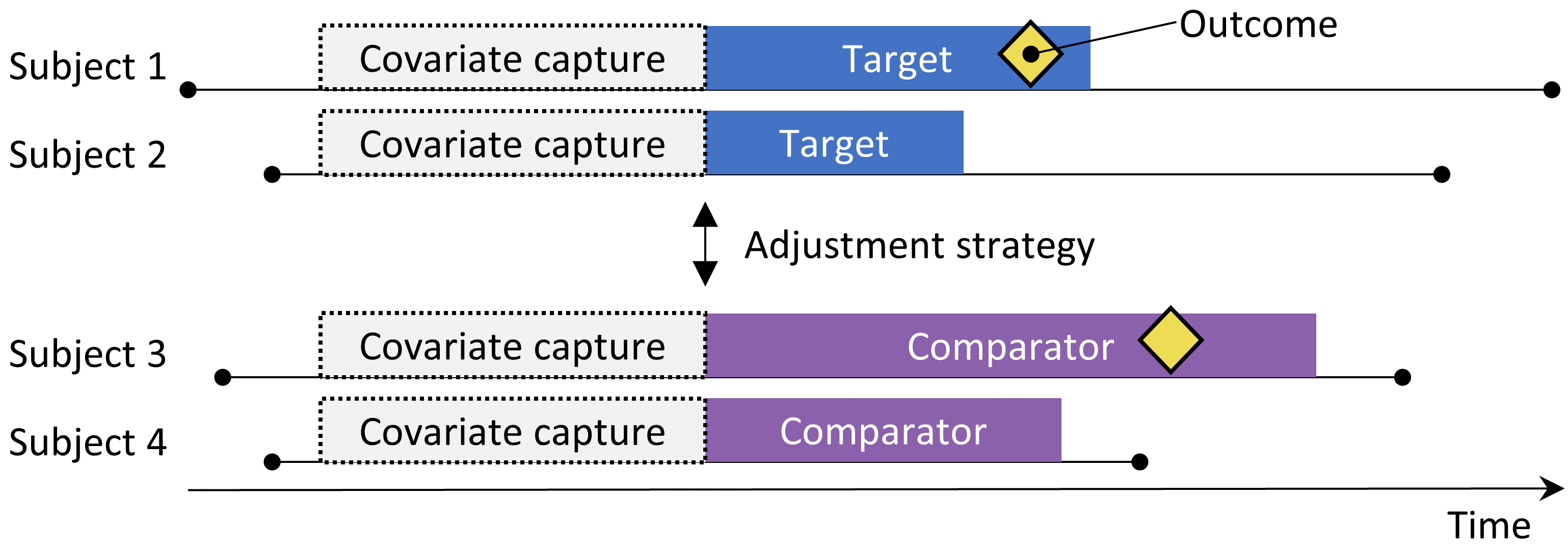
The new-user cohort design.
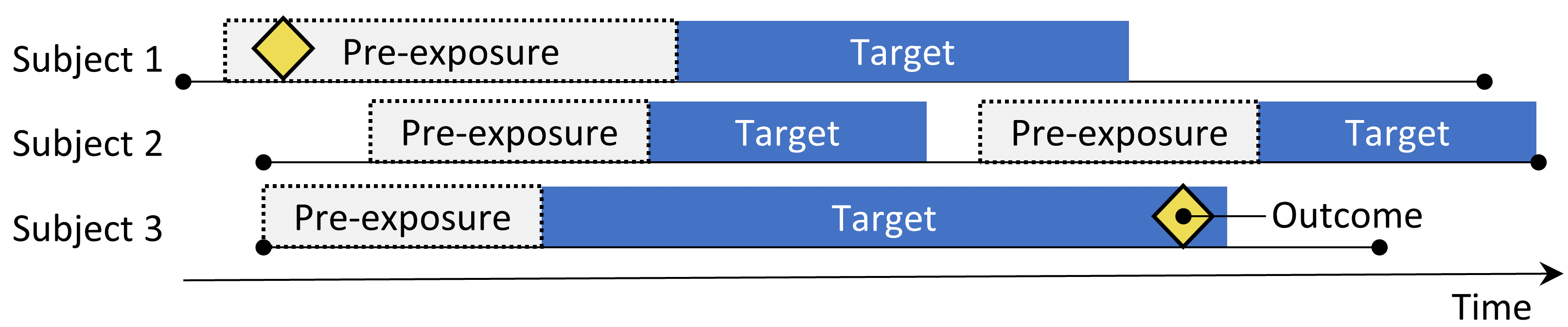
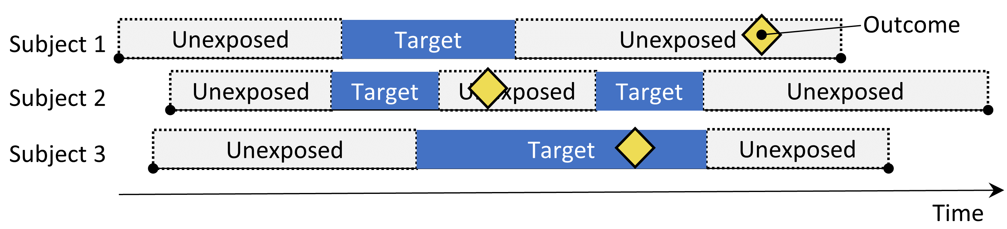
The self-controlled cohort design. The rate of outcomes during exposure to the target is compared to the rate of outcomes in the time pre-exposure.
The self-controlled cohort design. The rate of outcomes during exposure to the target is compared to the rate of outcomes in the time pre-exposure.
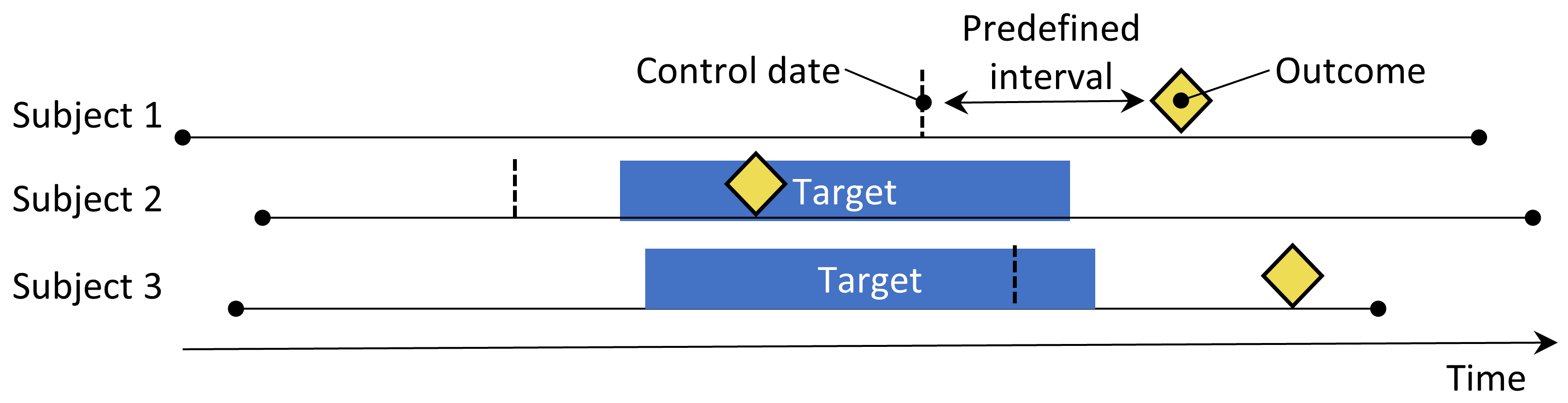
The case-crossover design. The time around the outcome is compared to a control date set at a predefined interval prior to the outcome date.
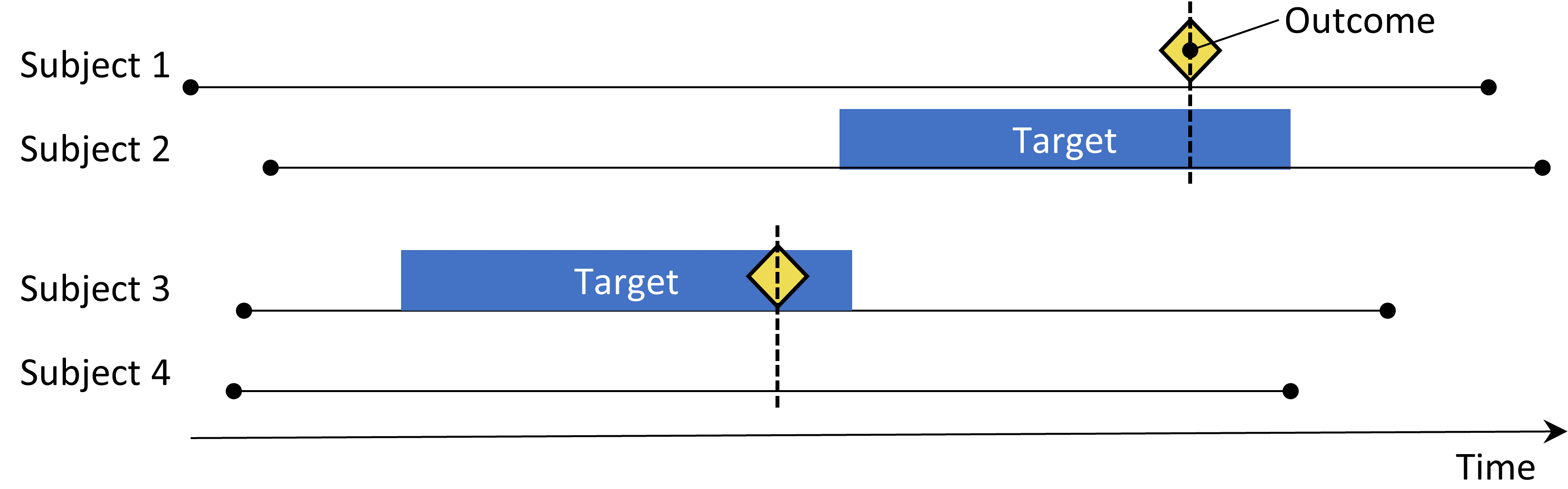
The Self-Controlled Case Series design. The rate of outcomes during exposure is compared to the rate of outcomes when not exposed.
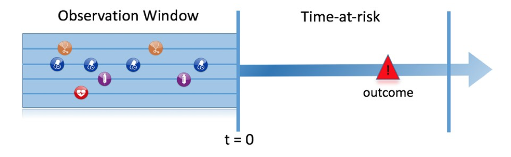
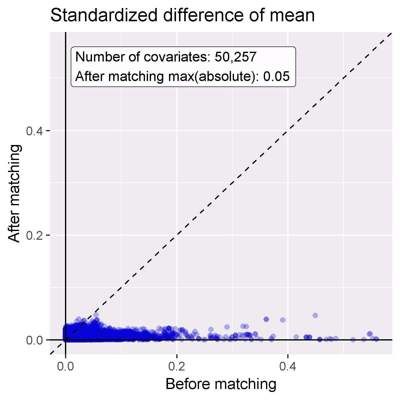
The prediction problem.