---
title: "Classification (ISL 4)"
subtitle: "Econ 425T"
author: "Dr. Hua Zhou @ UCLA"
date: "`r format(Sys.time(), '%d %B, %Y')`"
format:
html:
theme: cosmo
number-sections: true
toc: true
toc-depth: 4
toc-location: left
code-fold: false
engine: knitr
knitr:
opts_chunk:
fig.align: 'center'
# fig.width: 6
# fig.height: 4
message: FALSE
cache: false
---
Credit: This note heavily uses material from the books [_An Introduction to Statistical Learning: with Applications in R_](https://www.statlearning.com/) (ISL2) and [_Elements of Statistical Learning: Data Mining, Inference, and Prediction_](https://hastie.su.domains/ElemStatLearn/) (ESL2).
Display system information for reproducibility.
::: {.panel-tabset}
## Python
```{python}
import IPython
print(IPython.sys_info())
```
## R
```{r}
sessionInfo()
```
:::
## Overview of classification
- Qualitative variables take values in an unordered set $\mathcal{C}$,
such as: $\text{eye color} \in \{\text{brown}, \text{blue}, \text{green}\}$.
- Given a feature vector $X$ and a qualitative response $Y$
taking values in the set $\mathcal{C}$, the classification task is to build
a function $C(X)$ that takes as input the feature vector $X$ and predicts its value for $Y$, i.e. $C(X) \in \mathcal{C}$.
- Often we are more interested in estimating the probabilities that $X$ belongs to each category in $\mathcal{C}$.
## Credit `Default` data
- Response variable: Credit `default` (`yes` or `no`).
- Predictors:
- `balance`: credit card balance.
- `income`: income of customer.
- `student`: customer is a student or not.
::: {.panel-tabset}
#### Python
```{python}
# Load the pandas library
import pandas as pd
# Load numpy for array manipulation
import numpy as np
# Load seaborn plotting library
import seaborn as sns
import matplotlib.pyplot as plt
# Set font sizes in plots
sns.set(font_scale = 1.2)
# Display all columns
pd.set_option('display.max_columns', None)
# Import Credit Default data
Default = pd.read_csv("../data/Default.csv")
Default
```
```{python}
# Visualize income ~ balance
plt.figure()
sns.relplot(
data = Default,
x = 'balance',
y = 'income',
hue = 'default',
style = 'default',
height = 10
).set(
xlabel = 'Balance',
ylabel = 'Income'
);
plt.show()
```
```{python}
# Visualize balance ~ default
plt.figure()
sns.boxplot(
data = Default,
x = 'default',
y = 'balance'
).set(
xlabel = 'Default',
ylabel = 'Balance'
);
plt.show()
```
```{python}
# Visualize income ~ default
plt.figure()
sns.boxplot(
data = Default,
x = 'default',
y = 'income'
).set(
xlabel = 'Default',
ylabel = 'Income'
);
plt.show()
```
```{python}
# Visualize student ~ default
plt.figure()
sns.countplot(
data = Default,
x = 'default',
hue = 'student'
).set(
xlabel = 'Default',
ylabel = 'Count'
);
plt.show()
```
#### R
```{r}
library(ISLR2)
library(GGally) # ggpairs function
library(tidyverse)
# Credit default data
Default <- as_tibble(Default) %>%
print(width = Inf)
# Visualization by pair plot
ggpairs(
data = Default,
mapping = aes(),
lower = list(continuous = "smooth", combo = "box", discrete = "ratio")
) +
labs(title = "Credit Default Data")
```
:::
## Linear vs logistic regression
- If we code `default` as
$$
Y = \begin{cases}
0 & \text{if No} \\
1 & \text{if Yes}
\end{cases},
$$
can we simply perform a linear regression of $Y$ on $X$ and classify as `Yes` if $\hat Y > 0.5$?
- Since $\operatorname{E}(Y \mid X = x) = \operatorname{Pr}(Y=1 \mid X = x)$, we might think that linear regression is perfect for this task.
- The issue is that linear regression may produce probabilities <0 or >1, which does not make sense.
::: {.panel-tabset}
#### Python
```{python}
#| label: fig-default-lm-vs-logisitc
#| fig-cap: "Predicted probabilities by linear regression (blue line) vs logistic regression (green line)."
#| code-fold: true
# 0-1 (No-Yes) coding
Default['y'] = (Default['default'] == 'Yes').astype(int)
# Linear regression fit vs logistic regression fit
plt.figure()
sns.regplot(
data = Default,
x = 'balance',
y = 'y',
label = 'Linear regression'
)
sns.regplot(
data = Default,
x = 'balance',
y = 'y',
logistic = True,
label = 'Logistic regression',
line_kws = {'color': 'g'}
).set(
xlabel = 'Balance',
ylabel = 'Probability of Default'
)
plt.show()
```
#### R
```{r}
#| code-fold: true
Default %>%
mutate(y = as.integer(default == "Yes")) %>%
ggplot(mapping = aes(x = balance, y = y)) +
geom_point() +
geom_smooth(
method = "lm",
color = "blue",
show.legend = TRUE
) +
geom_smooth(
method = "glm",
method.args = list(family = binomial),
color = "green",
show.legend = TRUE
) +
labs(
x = "Balance",
y = "Probability of Default"
)
```
:::
- Now suppose we have a response variable with three possible values. A patient presents at the emergency room, and we must classify them according to their symptoms.
$$
Y = \begin{cases}
1 & \text{if stroke} \\
2 & \text{if drug overdose} \\
3 & \text{if epileptic seizure}
\end{cases}.
$$
This coding suggests an ordering, and in fact implies that the difference between `stroke` and `drug overdose` is the same as between `drug overdose` and `epileptic seizure`.
Linear regression is not appropriate here. Multiclass Logistic Regression or Discriminant Analysis are more appropriate.
## Logistic regression
- Let's write
$$
p(X) = \operatorname{Pr}(Y = 1 \mid X)
$$
for short. Logistic regression assumes
$$
p(X) = \frac{e^{\beta_0 + \beta_1 X_1 + \cdots + \beta_p X_p}}{1 + e^{\beta_0 + \beta_1 X_1 + \cdots + \beta_p X_p}}.
$$
$p(X) \in [0, 1]$, no matter what values of $\beta_j$ and $X$ take.
- A bit of rearrangement gives
$$
\log \left( \frac{p(X)}{1 - p(X)} \right) = \beta_0 + \beta_1 X_1 + \cdots + \beta_p X_p.
$$
This monotone transformation is called the **log odds** or **logit** transformation of $p(X)$.
- We use maximum likelihood to estimate the parameters. That is find $\beta_0, \ldots, \beta_p$ that maximizes the *likelihood* function
$$
\ell(\beta_0, \ldots, \beta_p) = \prod_{i:y_i=1} p(x_i) \prod_{i: y_i = 0} [1 - p(x_i)].
$$
::: {.panel-tabset}
#### Python (sklearn)
```{python}
from sklearn.linear_model import LogisticRegression
from sklearn.preprocessing import OneHotEncoder
from sklearn.compose import make_column_transformer
from sklearn.pipeline import Pipeline
# Code student as numerical 0/1
col_tf = make_column_transformer(
# OHE transformer for categorical variables
(OneHotEncoder(drop = 'first'), ['student']),
remainder = 'passthrough'
)
X = Default[['student', 'balance', 'income']]
y = Default['default']
# Pipeline
pipe_logit = Pipeline(steps = [
("col_tf", col_tf),
("model", LogisticRegression())
])
# Fit logistic regression
logit_fit = pipe_logit.fit(X, y)
logit_fit
# Predicted labels from logistic regression
logit_pred = logit_fit.predict(X)
# Confusion matrix from the logistic regression
logit_cfm = pd.crosstab(
logit_pred,
y,
margins = True,
rownames = ['Predicted Default Stats'],
colnames = ['True Default Status']
)
logit_cfm
```
Overall training accuracy of logistic regression (using 0.5 as threshold) is
```{python}
(logit_cfm.loc['Yes', 'Yes'] + logit_cfm.loc['No', 'No']) / logit_cfm.loc['All', 'All']
```
The area-under-ROC curve (AUC) of logistic regression (sklearn) is
```{python}
from sklearn.metrics import roc_auc_score
logit_auc = roc_auc_score(
y,
logit_fit.predict_proba(X)[:, 1]
)
logit_auc
```
#### Python (statsmodels)
```{python}
import statsmodels.api as sm
import statsmodels.formula.api as smf
# Fit logistic regression
logit_mod = smf.logit(
formula = 'y ~ balance + income + student',
data = Default
).fit()
logit_mod.summary()
# Predicted labels from logistic regression
logit_smpred = np.where(logit_mod.predict(X) > 0.5, 'Yes', 'No')
# Confusion matrix from the logistic regression
logit_smcfm = pd.crosstab(
logit_smpred,
y,
margins = True,
rownames = ['Predicted Default Stats'],
colnames = ['True Default Status']
)
```
Overall accuracy of logistic regression (by statsmodels)
```{python}
(logit_smcfm.loc['Yes', 'Yes'] + logit_smcfm.loc['No', 'No']) / logit_smcfm.loc['All', 'All']
```
The area-under-ROC curve (AUC) of logistic regression (statsmodels) is
```{python}
logit_smauc = roc_auc_score(
y,
logit_mod.predict(X)
)
logit_smauc
```
#### R
```{r}
library(gtsummary)
logit_mod <- glm(
default ~ balance + income + student,
family = binomial,
data = Default
)
summary(logit_mod)
# logit_mod %>% tbl_regression()
# Predicted labels from logistic regression
logit_pred = ifelse(
predict(logit_mod, Default, type = "response") > 0.5,
"Yes",
"No"
)
# Confusion matrix
logit_cfm = table(Predicted = logit_pred, Default = Default$default)
# Accuracy
(logit_cfm['Yes', 'Yes'] + logit_cfm['No', 'No']) / sum(logit_cfm)
```
:::
- We interpret the logistic regression coefficient as the expected change in log odds associated with one-unit increase in the corresponding predictor.
- Wait! Why the coefficient of `student` is negative, contradicting with the plot?
- **Confounding:** `student` status is confounded with `balance`. Students tend to have higher balances than non-students, so their marginal default rate is higher than for non-students.
But for each level of balance, students default less than non-students.
Multiple logistic regression can tease this out.
::: {.panel-tabset}
#### Python
::: {#fig-default-confounding}
```{python}
#| code-fold: true
# Visualize balance ~ default
plt.figure()
sns.boxplot(
data = Default,
x = 'student',
y = 'balance'
).set(
xlabel = 'Student Status',
ylabel = 'Credit Card Balance'
);
plt.show()
```
```{python}
#| code-fold: true
# Add predicted probabilities to DataFrame
Default['yhat'] = logit_mod.predict()
# Visualize yhat ~ balance
plt.figure()
sns.relplot(
data = Default,
x = 'balance',
y = 'yhat',
kind = 'line',
hue = 'student',
height = 8
).set(
xlabel = 'Credit Card Balance',
ylabel = 'Default Rate'
);
plt.show()
```
Student status confounds with credit card balance. Students tend to have higher balances than non-students. Even though students default less at than non-students for each level of balance, marginally their default rate is higher than for non-students.
:::
#### R
```{r}
#| code-fold: true
ggplot(data = Default) +
geom_boxplot(mapping = aes(x = student, y = balance)) +
labs(
x = "Student Status",
y = "Credit Card Balance",
title = "Students tend to carry larger credit card balance."
)
Default %>%
mutate(yhat = logit_mod$fitted.values) %>%
ggplot() +
geom_point(mapping = aes(x = balance, y = yhat, color = student)) +
labs(
x = "Credit Card Balance",
y = "Default Rate",
subtitle = "Even though students default less at than non-students for each level of balance, marginally their default rate is higher than for non-students."
)
```
:::
## Multinomial logit regression
For more than two classes, we generalize logistic regression to
$$
\operatorname{Pr}(Y = k \mid X) = \frac{e^{\beta_{0k} + \beta_{1k} X_1 + \cdots + \beta_{pk} X_p}}{\sum_{\ell = 1}^K e^{\beta_{0\ell} + \beta_{1\ell} X_1 + \cdots + \beta_{p\ell} X_p}}.
$$
Note each class has its own set of regression coefficients.
In Python, we can fit multinomial logit model by [`statsmodels.discrete.discrete_model.MNLogit`](https://www.statsmodels.org/dev/generated/statsmodels.discrete.discrete_model.MNLogit.html). In R, we can use `glmnet` package or `nnet` package.
## Discriminant analysis
- Another approach for classification is to model the distribution of $X$ in each of the classes separately, and then use **Bayes theorem** to flip things around and obtain $\operatorname{Pr}(Y = j \mid X)$.
- When we use normal (Gaussian) distributions for each class, this leads to linear or quadratic discriminant analysis.
- However, this approach is quite general, and other distributions can be used as well. We will focus on normal distributions.
- [Thomas Bayes](https://en.wikipedia.org/wiki/Thomas_Bayes) was a famous mathematician whose name represents a big subfield of statistical and probabilistic modeling. Here we focus on a simple result, known as **Bayes theorem**:
\begin{eqnarray*}
p_k(x) &=& \operatorname{Pr}(Y = k \mid X = x) \\
&=& \frac{\operatorname{Pr}(X = x, Y = k)}{\operatorname{Pr}(X = x)} \\
&=& \frac{\operatorname{Pr}(X = x \mid Y = k) \cdot \operatorname{Pr}(Y = k)}{\operatorname{Pr}(X = x)} \\
&=& \frac{\pi_k f_k(x)}{\sum_{\ell=1}^K \pi_\ell f_\ell(x)},
\end{eqnarray*}
where
- $f_k(x) = \operatorname{Pr}(X = x \mid Y = k)$ is the density of $X$ in class $k$
- $\pi_k = \operatorname{Pr}(Y = k)$ is the marginal or **prior** probability for class $k$.
- Advantages of discriminant analysis.
- When the classes are well-separated, the parameter estimates for the logistic regression model are surprisingly unstable (separation or quasi-separation). Linear discriminant analysis does not suffer from this problem.
- If $n$ is small and the distribution of the predictors $X$ is approximately normal in each of the classes, the linear discriminant model is again more stable than the logistic regression model.
### Linear discriminant analysis (LDA)
- Assume $X \in \mathbb{R}^p$ in the $k$-th class is distributed as as multivariate normal $N(\mu_k, \boldsymbol{\Sigma})$ with density
$$
f_k(x) = \frac{1}{(2\pi)^{p/2} |\boldsymbol{\Sigma}|^{1/2}} e^{- \frac{1}{2} (x - \mu_k)^T \boldsymbol{\Sigma}^{-1} (x - \mu_k)}.
$$
To classify $X=x$, we need to see which of $p_k(x)$ is small. Taking logs, and discarding terms that do not depend on $k$, we just need to assign $x$ to the class with the largest **discriminant score**
$$
\delta_k(x) = x^T \boldsymbol{\Sigma}^{-1} \mu_k - \frac{1}{2} \mu_k^T \boldsymbol{\Sigma}^{-1} \mu_k + \log \pi_k,
$$
which is a linear function in $x$!
- We estimate the unknown parameters $\pi_k$, $\mu_k$, and $\boldsymbol{\Sigma}$ by
\begin{eqnarray*}
\hat{\pi}_k &=& \frac{n_k}{n} \\
\hat{\mu}_k &=& \frac{1}{n_k} \sum_{i: y_k = k} x_i \\
\hat{\boldsymbol{\Sigma}} &=& \frac{1}{n-K} \sum_{k=1}^K \sum_{i: y_i = k} (x_i - \hat \mu_k)(x_i - \hat \mu_k)^T.
\end{eqnarray*}
- Once we have estimated $\hat \delta_k(x)$, we can turn these into class probabilities
$$
\hat{\operatorname{Pr}}(Y = k \mid X = x) = \frac{e^{\hat \delta_k(x)}}{\sum_{\ell=1}^K e^{\hat \delta_{\ell}(x)}}.
$$
::: {#fig-tradeoff-truth}
{width=700px height=350px}
Here $\pi_1 = \pi_2 = \pi_3 = 1/3$. The dashed lines are known as the Bayes decision boundaries. Were they known, they would yield the fewest misclassification errors, among all possible classifiers. The black line is the LDA decision boundary.
:::
- LDA on the credit `Default` data.
::: {.panel-tabset}
#### Python
```{python}
from sklearn.discriminant_analysis import LinearDiscriminantAnalysis
# Pipeline
pipe_lda = Pipeline(steps = [
("col_tf", col_tf),
("model", LinearDiscriminantAnalysis())
])
# Fit LDA
lda_fit = pipe_lda.fit(X, y)
# Predicted labels from LDA
lda_pred = lda_fit.predict(X)
# Confusion matrix
lda_cfm = pd.crosstab(
lda_pred,
y,
margins = True,
rownames = ['Predicted Default Stats'],
colnames = ['True Default Status']
)
lda_cfm
```
Overall training accuracy of LDA (using 0.5 as threshold) is
```{python}
(lda_cfm.loc['Yes', 'Yes'] + lda_cfm.loc['No', 'No']) / lda_cfm.loc['All', 'All']
```
The area-under-ROC curve (AUC) of LDA is
```{python}
lda_auc = roc_auc_score(
y,
lda_fit.predict_proba(X)[:, 1]
)
lda_auc
```
#### R
```{r}
library(MASS)
# Fit LDA
lda_mod <- lda(
default ~ balance + income + student,
data = Default
)
lda_mod
# Predicted labels from LDA
lda_pred = predict(lda_mod, Default)
# Confusion matrix
lda_cfm = table(Predicted = lda_pred$class, Default = Default$default)
# Accuracy
(lda_cfm['Yes', 'Yes'] + lda_cfm['No', 'No']) / sum(lda_cfm)
```
:::
### Quadratic discriminant analysis (QDA)
- In LDA, the normal distribution for each class shares the same covariance $\boldsymbol{\Sigma}$.
- If we assume that the normal distribution for class $k$ has covariance $\boldsymbol{\Sigma}_k$, then it leads to the **quadratic discriminant analysis** (QDA).
- The discriminant function takes the form
$$
\delta_k(x) = - \frac{1}{2} (x - \mu_k)^T \boldsymbol{\Sigma}_k^{-1} (x - \mu_k) + \log \pi_k - \frac{1}{2} \log |\boldsymbol{\Sigma}_k|,
$$
which is a quadratic function in $x$.
::: {#fig-lda-vs-qda}
{width=700px height=350px}
The Bayes (purple dashed), LDA (black dotted), and QDA (green solid) decision boundaries for a two-class problem. Left: $\boldsymbol{\Sigma}_1 = \boldsymbol{\Sigma}_2$. Right: $\boldsymbol{\Sigma}_1 \ne \boldsymbol{\Sigma}_2$.
:::
::: {.panel-tabset}
#### Python
```{python}
from sklearn.discriminant_analysis import QuadraticDiscriminantAnalysis
# Pipeline
pipe_qda = Pipeline(steps = [
("col_tf", col_tf),
("model", QuadraticDiscriminantAnalysis())
])
# Fit QDA
qda_fit = pipe_qda.fit(X, y)
# Predicted labels from QDA
qda_pred = qda_fit.predict(X)
# Confusion matrix from the QDA
qda_cfm = pd.crosstab(
qda_pred,
y,
margins = True,
rownames = ['Predicted Default Stats'],
colnames = ['True Default Status']
)
qda_cfm
```
Overall training accuracy of QDA (using 0.5 as threshold) is
```{python}
(qda_cfm.loc['Yes', 'Yes'] + qda_cfm.loc['No', 'No']) / qda_cfm.loc['All', 'All']
```
The area-under-ROC curve (AUC) of QDA is
```{python}
qda_auc = roc_auc_score(
y,
qda_fit.predict_proba(X)[:, 1]
)
qda_auc
```
#### R
```{r}
# Fit QDA
qda_mod <- qda(
default ~ balance + income + student,
data = Default
)
qda_mod
# Predicted probabilities from QDA
qda_pred = predict(qda_mod, Default)
# Confusion matrix
qda_cfm = table(Predicted = qda_pred$class, Default = Default$default)
# Accuracy
(qda_cfm['Yes', 'Yes'] + qda_cfm['No', 'No']) / sum(qda_cfm)
```
:::
### Naive Bayes
- If we assume $f_k(x) = \prod_{j=1}^p f_{jk}(x_j)$ (conditional independence model) in each class, we get **naive Bayes**.
For Gaussian this means the $\boldsymbol{\Sigma}_k$ are diagonal.
- Naive Bayes is useful when $p$ is large (LDA and QDA break down).
- Can be used for $mixed$ feature vectors (both continuous and categorical). If $X_j$ is qualitative, replace $f_{kj}(x_j)$ with probability mass function (histogram) over discrete
categories.
- Despite strong assumptions, naive Bayes often produces good classification results.
::: {.panel-tabset}
#### Python
```{python}
from sklearn.naive_bayes import GaussianNB
# Pipeline
pipe_nb = Pipeline(steps = [
("col_tf", col_tf),
("model", GaussianNB())
])
# Fit Naive Bayes classifier
nb_fit = pipe_nb.fit(X, y)
# Predicted labels by NB classifier
nb_pred = nb_fit.predict(X)
# Confusion matrix of NB classifier
nb_cfm = pd.crosstab(
nb_pred,
y,
margins = True,
rownames = ['Predicted Default Stats'],
colnames = ['True Default Status']
)
nb_cfm
```
Overall training accuracy of Naive Bayes classifier (using 0.5 as threshold) is
```{python}
(nb_cfm.loc['Yes', 'Yes'] + nb_cfm.loc['No', 'No']) / nb_cfm.loc['All', 'All']
```
The area-under-ROC curve (AUC) of NB is
```{python}
nb_auc = roc_auc_score(
y,
nb_fit.predict_proba(X)[:, 1]
)
nb_auc
```
#### R
```{r}
library(e1071)
# Fit Naive Bayes classifier
nb_mod <- naiveBayes(
default ~ balance + income + student,
data = Default
)
nb_mod
# Predicted labels from Naive Bayes
nb_pred = predict(nb_mod, Default)
# Confusion matrix
nb_cfm = table(Predicted = nb_pred, Default = Default$default)
# Accuracy
(nb_cfm['Yes', 'Yes'] + nb_cfm['No', 'No']) / sum(nb_cfm)
```
:::
## $K$-nearest neighbor (KNN) classifier
- KNN is a nonparametric classifier.
- Given a positive integer $K$ and a test observation $x_0$, the KNN classifier first identifies the $K$ points in the training data that are closest to $x_0$, represented by $\mathcal{N}_0$. It estimates the conditional probability by
$$
\operatorname{Pr}(Y=j \mid X = x_0) = \frac{1}{K} \sum_{i \in \mathcal{N}_0} I(y_i = j)
$$
and then classifies the test observation $x_0$ to the class with the largest probability.
- We illustrate KNN with $K=5$ on the credit default data.
::: {.panel-tabset}
#### Python
```{python}
from sklearn.neighbors import KNeighborsClassifier
# Pipeline
pipe_knn = Pipeline(steps = [
("col_tf", col_tf),
("model", KNeighborsClassifier(n_neighbors = 5))
])
# Fit KNN with K = 5
knn_fit = pipe_knn.fit(X, y)
# Predicted labels from KNN
knn_pred = knn_fit.predict(X)
# Confusion matrix of KNN
knn_cfm = pd.crosstab(
knn_pred,
y,
margins = True,
rownames = ['Predicted Default Stats'],
colnames = ['True Default Status']
)
knn_cfm
```
Overall training accuracy of KNN classifier with $K=5$ (using 0.5 as threshold) is
```{python}
(knn_cfm.loc['Yes', 'Yes'] + knn_cfm.loc['No', 'No']) / knn_cfm.loc['All', 'All']
```
The area-under-ROC curve (AUC) of KNN ($K=5$) is
```{python}
knn_auc = roc_auc_score(
y,
knn_fit.predict_proba(X)[:, 1]
)
knn_auc
```
#### R
```{r}
library(class)
X_default <- Default %>%
mutate(x_student = as.integer(student == "Yes")) %>%
dplyr::select(x_student, balance, income)
# KNN prediction with K = 5
knn_pred <- knn(
train = X_default,
test = X_default,
cl = Default$default,
k = 5
)
# Confusion matrix
knn_cfm = table(Predicted = knn_pred, Default = Default$default)
# Accuracy
(knn_cfm['Yes', 'Yes'] + knn_cfm['No', 'No']) / sum(knn_cfm)
```
:::
## Evaluation of classification performance: false positive, false negative, ROC and AUC
- Let's summarize the classification performance of different classifiers on the training data.
::: {.panel-tabset}
#### Python
```{python}
# Confusion matrix from the null classifier (always 'No')
null_cfm = pd.DataFrame(
data = {
'No': [9667, 0, 9667],
'Yes': [333, 0, 333],
'All': [10000, 0, 10000]
},
index = ['No', 'Yes', 'All']
)
null_pred = np.repeat('No', 10000)
# Fitted classifiers
classifiers = [logit_fit, lda_fit, qda_fit, nb_fit, knn_fit]
# Confusion matrices
cfms = [logit_cfm, lda_cfm, qda_cfm, nb_cfm, knn_cfm, null_cfm]
```
```{python}
sm_df = pd.DataFrame(
data = {
'acc': [(cfm.loc['Yes', 'Yes'] + cfm.loc['No', 'No']) / cfm.loc['All', 'All'] for cfm in cfms],
'fpr': [(cfm.loc['Yes', 'No'] / cfm.loc['All', 'No']) for cfm in cfms],
'fnr': [(cfm.loc['No', 'Yes'] / cfm.loc['All', 'Yes']) for cfm in cfms],
'auc': np.append([roc_auc_score(y, c.predict_proba(X)[:, 1]) for c in classifiers], roc_auc_score(y, np.repeat(0, 10000)))
},
index = ['logit', 'LDA', 'QDA', 'NB', 'KNN', 'Null']
)
sm_df.sort_values('acc')
```
#### R
:::
- There are two types of classification errors:
- **False positive rate**: The fraction of negative examples that are classified as positive.
- **False negative rate**: The fraction of positive examples that are classified as negative.
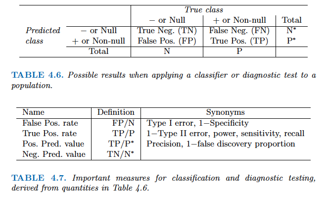
- Above table is the training classification performance of classifiers using their default thresholds. Varying thresholds lead to varying false positive rates (1 - specificity) and true positive rates (sensitivity). These can be plotted as the **receiver operating characteristic (ROC)** curve. The overall performance of a classifier is summarized by the **area under ROC curve (AUC)**.
```{python}
from sklearn.metrics import roc_curve
from sklearn.metrics import RocCurveDisplay
# plt.rcParams.update({'font.size': 12})
for idx, m in enumerate(classifiers):
plt.figure();
RocCurveDisplay.from_estimator(m, X, y, name = sm_df.iloc[idx].name);
plt.show()
# ROC curve of the null classifier (always No or always Yes)
plt.figure()
RocCurveDisplay.from_predictions(y, np.repeat(0, 10000), pos_label = 'Yes', name = 'Null Classifier');
plt.show()
```
- See [sklearn.metrics](https://scikit-learn.org/stable/modules/model_evaluation.html) for other popularly used metrics for classification tasks.
## Comparison between classifiers
- For a two-class problem, we can show that for LDA,
$$
\log \left( \frac{p_1(x)}{1 - p_1(x)} \right) = \log \left( \frac{p_1(x)}{p_2(x)} \right) = c_0 + c_1 x_1 + \cdots + c_p x_p.
$$
So it has the same form as logistic regression. The difference is in how the parameters are estimated.
- Logistic regression uses the conditional likelihood based on $\operatorname{Pr}(Y \mid X)$ (known as **discriminative learning**).
LDA, QDA, and Naive Bayes use the full likelihood based on $\operatorname{Pr}(X, Y)$ (known as **generative learning**).
- Despite these differences, in practice the results are often very similar.
- Logistic regression can also fit quadratic boundaries like QDA, by explicitly including quadratic terms in the model.
- Logistic regression is very popular for classification, especially when $K = 2$.
- LDA is useful when $n$ is small, or the classes are well separated, and Gaussian assumptions are reasonable. Also when $K > 2$.
- Naive Bayes is useful when $p$ is very large.
- LDA is a special case of QDA.
- Under normal assumption, Naive Bayes leads to linear decision boundary, thus a special case of LDA.
- KNN classifier is non-parametric and can dominate LDA and logistic regression when the decision boundary is highly nonlinear, provided that $n$ is very large and $p$ is small.
- See ISL Section 4.5 for theoretical and empirical comparisons of logistic regression, LDA, QDA, NB, and KNN.