{width=400px height=400px}
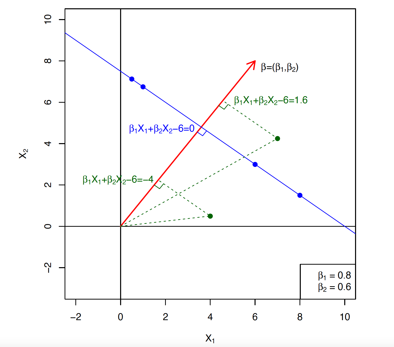
Hyperplane in 2 dimensions. ::: - If $\beta_0 = 0$, the hyperplane goes through the origin, otherwise not. - The vector $\beta = (\beta_1, \ldots, \beta_p)$ is called the normal vector. It points in a direction orthogonal to the surface of hyperplane. That is $$ \beta^T (x_1 - x_2) = 0 $$ for any two points $x_1, x_2$ in the hyperplane. - If $$ f(X) = \beta_0 + \beta_1 X_1 + \cdots + \beta_p X_p = \beta_0 + \beta^T X, $$ then $f(X) > 0$ for points on one side of the hyperplane, and $f(X) < 0$ for points on the other. For any $x_0$ in the hyperplane $f(x)=0$, $\beta^T x_0 = - \beta_0$. The signed distance of any point $x$ to the hyperplane $f(x)=0$ is given by $$ \frac{1}{\|\beta\|} (\beta^T x - \beta^T x_0) = \frac{1}{\|\beta\|} (\beta^T x + \beta_0) = \frac{1}{\|\beta\|} f(x), $$ where $$ \|\beta\|=\sqrt{\sum_{j=1}^p \beta_j^2}. $$ Thus $f(x)$ is proportional to the signed distance from $x$ to the hyperplane defined by $f(x) = 0$. - If we code the colored points as $y_i = +1$ for blue, say and $y_i = -1$ for mauve, then if $y_i \cdot f(X_i) > 0$ for all $i$, $f(X) = 0$ defines a **separating hyperplane**. ::: {#fig-separating-hyperplane}{width=600px height=375px}
Left: There are two classes of observations, shown in blue and in purple, each of which has measurements on two variables. Three separating hyperplanes, out of many possible, are shown in black. Right: A separating hyperplane is shown in black. The blue and purple grid indicates the decision rule made by a classifier based on this separating hyperplane: a test observation that falls in the blue portion of the grid will be assigned to the blue class, and a test observation that falls into the purple portion of the grid will be assigned to the purple class. ::: ## Maximal margin classifier - Among all separating hyperplanes, find the one that makes the biggest gap or margin between the two classes. ::: {#fig-max-margin-classifier}{width=400px height=450px}
The maximal margin hyperplane is shown as a solid line. The margin is the distance from the solid line to either of the dashed lines. The two blue points and the purple point that lie on the dashed lines are the **support vectors**, and the distance from those points to the hyperplane is indicated by arrows. The purple and blue grid indicates the decision rule made by a classifier based on this separating hyperplane. ::: - Constrained optimization: \begin{eqnarray*} \max\limits_{\beta_0,\beta_1,\ldots,\beta_p, M} & & \quad M \\ \text{subject to} & & \sum_{j=1}^p \beta_j^2 = 1 \\ & & y_i (\beta_0 + \beta^T x_i) \ge M \text{ for all } i. \end{eqnarray*} The constraints ensure that each observation is on the correct side of the hyperplane and at least a distance $M$ from the hyperplane. - We can get rid of the $\|\beta\|^2 = 1$ constraint by replacing the inequality by $$ \frac{1}{\|\beta\|^2} y_i (\beta_0 + \beta^T x_i) \ge M, $$ (which redefines $\beta_0$) or equivalently $$ y_i (\beta_0 + \beta^T x_i) \ge M \|\beta\|^2. $$ Since for any $\beta_0,\beta_1,\ldots,\beta_p$ satisfying these inequalities, any positively scaled multiple satisfies them too, we can arbitrarily set $\|\beta\|^2 = 1/M$. - Thus we equivalently solve \begin{eqnarray*} \min_{\beta_0,\beta_1,\ldots,\beta_p} & & \frac 12 \|\beta\|^2 \\ \text{subject to} & & y_i (\beta_0 + \beta^T x_i) \ge 1, \quad i = 1,\ldots,n. \end{eqnarray*} This is a quadratic optimization problem. Intuitively, the constraints define an empty slab or margin around the linear decision boundary of thickness $1/\|\beta\|^2$. Hence we choose $\beta_0,\beta_1,\ldots,\beta_p$ to maximize its thickness. - The Lagrange (primal) function is $$ L_P = \frac 12 \|\beta\|^2 - \sum_{i=1}^n \alpha_i [y_i (x_i^T \beta + \beta_0) - 1]. $$ Setting the derivatives (with respect to $\beta$ and $\beta_0$) to zero, we obtain $$ \beta = \sum_{i=1}^n \alpha_i y_i x_i $$ {#eq-svm-primal-stationary-condition} $$ 0 = \sum_{i=1}^n \alpha_i y_i, $$ and substituting these to the $L_p$ we obtained the dual \begin{eqnarray*} \max_{\alpha_1,\ldots,\alpha_n} & & L_D = \sum_{i=1}^n \alpha_i - \frac 12 \sum_{i=1}^n \sum_{i'=1}^n \alpha_i \alpha_{i'} y_i y_{i'} x_i^T x_{i'} \\ \text{subject to} & & \alpha_i \ge 0, \sum_{i=1}^n \alpha_i y_i = 0. \end{eqnarray*} The solution $\alpha_i$ must satisfy the so-called complimentary slackness condition $$ \alpha_i [y_i (\beta_0 + \beta^T x_i) - 1] = 0 \quad i=1,\ldots,n. $$ Thus - if $\alpha_i>0$, then $y_i (\beta_0 + \beta^T x_i) = 1$, or in other words, $x_i$ is on the boundary of the slab; - if $y_i (\beta_0 + \beta^T x_i) > 1$, $x_i$ is not on the boundary of the slab, and $\alpha_i=0$. Hence the solution $\beta$ only depends on the support vectors with $\alpha_i > 0$. ## Support vector classifier (soft margin classifier) - Non-separable data. Sometimes the data are not separable by a linear boundary. This if often the case, unless $N < p$. ::: {#fig-noisy-data}{width=400px height=450px}
The two classes are not separable by a hyperplane, and so the maximal margin classifier cannot be used. ::: - Noisy data. Sometimes the data are separable, but noisy. This can lead to a poor solution for the maximal margin classifier.{width=600px height=350px}
- The **support vector classifier** maximizes a **soft** margin. \begin{eqnarray*} \max\limits_{\beta_0,\beta_1,\ldots,\beta_p, \epsilon_1, \ldots, \epsilon_n, M} & & \quad M \\ \text{subject to} & & \sum_{j=1}^p \beta_j^2 = 1 \\ & & y_i (\beta_0 + \beta^T x_i) \ge M (1-\epsilon_i) \\ & & \epsilon_i \ge 0, \sum_{i=1}^n \epsilon_i \le C. \end{eqnarray*} $M$ is the width of the margin. - $\epsilon_1, \ldots, \epsilon_n$ are **slack variables** that allow individual observations to be on the wrong side of the margin or the hyperplane. - If $\epsilon_i = 0$, then the $i$-th observation is on the correct side of the margin. - If $0 < \epsilon_i \le 1$, then the $i$-th observation is on the wrong side of the margin. - If $\epsilon_i > 1$, then the $i$-th observation is on the wrong side of the hyperplane. ::: {#fig-soft-margin-classifier}{width=600px height=350px}
Left: A support vector classifier was fit to a small data set. The hyperplane is shown as a solid line and the margins are shown as dashed lines. Purple observations: Observations 3, 4, 5, and 6 are on the correct side of the margin, observation 2 is on the margin, and observation 1 is on the wrong side of the margin. Blue observations: Observations 7 and 10 are on the correct side of the margin, observation 9 is on the margin, and observation 8 is on the wrong side of the margin. No observations are on the wrong side of the hyperplane. Right: Same as left panel with two additional points, 11 and 12. These two observations are on the wrong side of the hyperplane and the wrong side of the margin. ::: - $C$ is a regularization parameter that controls the amount that the margin can be violated by the $n$ observations. $C$ controls the bias-variance trade-off. ::: {#fig-C}{width=600px height=600px}
The largest value of $C$ was used in the top left panel, and smaller values were used in the top right, bottom left, and bottom right panels. When $C$ is large, then there is a high tolerance for observations being on the wrong side of the margin, and so the margin will be large. As $C$ decreases, the tolerance for observations being on the wrong side of the margin decreases, and the margin narrows. ::: - By a similar reparameterization trick as before, we solve the equivalent optimization problem \begin{eqnarray*} \min & & \frac 12 \|\beta\|^2 \\ \text{subject to} & & y_i(\beta_0 + \beta^T x_i) \ge 1 - \xi_i, \quad i=1,\ldots,n \\ & & \xi_i \ge 0, \sum_i \xi_i \le \text{constant}. \end{eqnarray*} - The dual is (derivation omitted) \begin{eqnarray*} \max_{\alpha_1,\ldots,\alpha_n} & & L_D = \sum_{i=1}^n \alpha_i - \frac 12 \sum_{i=1}^n \sum_{i'=1}^n \alpha_i \alpha_{i'} y_i y_{i'} x_i^T x_{i'} \\ \text{subject to} & & 0 \le \alpha_i \le C, \sum_{i=1}^n \alpha_i y_i = 0. \end{eqnarray*} ## Nonlinearity: support vector machines (SVM) - Sometime a linear boundary simply won't work, no matter what value of $C$. ::: {#fig-nonlinear-data}{width=600px height=400px}
Left: The observations fall into two classes, with a non-linear boundary between them. Right: The support vector classifier seeks a linear boundary, and consequently performs very poorly. ::: - Enlarge the space of features by including transformations: $X_1^2, X_1^3, X_1 X_2, X_1 X_2^2, \ldots$ Hence go from a $p$-dimensional space to an $M > p$ dimensional space. $$ \beta_0 + \beta_1 X_1 + \beta_2 X_2 + \beta_3 X_1^2 + \beta_4 X_2^2 + \beta_5 X_1 X_2 + \beta_6 X_1^3 + \beta_7 X_2^3 + \beta_8 X_1 X_2^2 + \beta_9 X_1^2 X_2 = 0. $$ ## Kernels - Polynomials (especially high-dimensional ones) get wild rather fast (too many features). - There is a more elegant and controlled way to introduce nonlinearities in support-vector classifiers through the use of **kernels**. - **Inner product** between two vectors: $$ \langle x_i, x_{i'} \rangle = \sum_{j=1}^p x_{ij} x_{i'j}. $$ - By (@eq-svm-primal-stationary-condition), the linear support vector classifier can be represented as $$ f(x) = \beta_0 + \sum_{i=1}^n \alpha_i y_i \langle x, x_i \rangle. $$ To estimate the parameters $\alpha_1,\ldots,\alpha_n$ and $\beta_0$, all we need are the $\binom{n}{2}$ inner products $\langle x_i, x_{i'} \rangle$ between all pairs of training observations. - It turns out that most of the $\hat \alpha_i$ (non-support vectors) can be zero: $$ \hat f(x) = \hat \beta_0 + \sum_{i \in \mathcal{S}} \hat \alpha_i y_i \langle x, x_i \rangle. $$ $\mathcal{S}$ is the **support set** of indices $i$ such that $\alpha_i > 0$. - If we can compute inner products between observations, we can fit a SV classifier. - Some special kernel functions can do this for us. E.g. the **polynomial kernel** of degree $d$ $$ K(x_i, x_{i'}) = \left(1 + \sum_{j=1}^p x_{ij} x_{i'j} \right)^d $$ computes the inner products needed for $d$-dimensional polynomials. For example, for degree $d=2$ and $p=2$ features, \begin{eqnarray*} K(x, x') &=& (1 + \langle x, x' \rangle)^2 \\ &=& 1 + 2x_1x_1' + 2 x_2 x_2' + (x_1x_1)^2 + (x_2x_2')^2 + 2x_1x_1'x_2x_2' \\ &=& \langle \begin{pmatrix} 1 \\ \sqrt{2} x_1 \\ \sqrt{2} x_2 \\ x_1^2 \\ x_2^2 \\ \sqrt{2} x_1 x_2 \end{pmatrix}, \begin{pmatrix} 1 \\ \sqrt{2} x_1' \\ \sqrt{2} x_2' \\ x_1^{'2} \\ x_2^{'2} \\ \sqrt{2} x_1' x_2' \end{pmatrix} \rangle \end{eqnarray*} is equivalent to inner product in a $M=6$ dimensional feature space. - The solution has the form $$ \hat f(x) = \hat \beta_0 + \sum_{i \in \mathcal{S}} \hat{\alpha}_i y_i K(x, x_i). $$ - **Radial kernel**: $$ K(x_i, x_{i'}) = \exp \left( - \gamma \sum_{j=1}^p (x_{ij} - x_{i'j})^2 \right). $$ The solution has the form $$ \hat f(x) = \hat \beta_0 + \sum_{i \in \mathcal{S}} \hat \alpha_i y_i K(x, x_i). $$ Implicit feature space is very high dimensional. Controls variance by squashing down most dimensions severely. The scale parameter $\gamma$ is tuned by cross-validation. ::: {#fig-nonlinear-svm}{width=600px height=400px}
Left: An SVM with a polynomial kernel of degree 3. Right: An SVM with a radial kernel. In this example, either kernel is capable of capturing the decision boundary. ::: ## `Heart` data example [Workflow: SVM with polynomial kernel](https://ucla-econ-425t.github.io/2023winter/slides/09-svm/workflow_svm_poly.html) [Workflow: SVM with radial kernel](https://ucla-econ-425t.github.io/2023winter/slides/09-svm/workflow_svm_rbf.html) ## SVM for more than 2 classes - What do we do if we have $K > 2$ classes? - **OVA**. One versus All. Fit $K$ different 2-class SVM classifiers $\hat f_k(x)$, $k=1,\ldots,K$; each class (coded as 1) versus the rest (coded as -1). Classify $x^*$ to the class for which $\hat f_k(x^*)$ is largest, as it indicates high level of confidence that the test observation belongs to the $k$th class rather than to any of the other classes. - **OVO**. One versus One. Fit all $\binom{K}{2}$ pairwise classifiers $\hat f_{k\ell}(x)$. Classify $x^*$ to the class that wins the most pairwise competitions. - Which to choose? If $K$ is not too large, use OVO. ## SVM vs logistic regression (LR) - With $f(X) = \beta_0 + \beta_1 X_1 + \cdots + \beta_p X_p$, the support vector classifier optimization can be recast as $$ \min\limits_{\beta_0,\beta_1,\ldots,\beta_p} \left\{ \sum_{i=1}^n \max[0, 1 - y_i f(x_i)] + \lambda \sum_{j=1}^p \beta_j^2 \right\}. $$ **Hinge loss** + **ridge penalty** - The hinge loss is very similar to the negative log-likelihood of the logistic regression.{width=400px height=400px}
- Which one to use? - When classes are (nearly) separable, SVM does better than LR. So does LDA. - When not, LR (with ridge penalty) and SVM very similar. - If you wish to estimate probabilities, LR is the choice. - For nonlinear boundaries, kernel SVMs are popular. Can use kernels with LR and LDA as well, but computations are more expensive.