 "
]
},
{
"cell_type": "markdown",
"metadata": {},
"source": [
"
"
]
},
{
"cell_type": "markdown",
"metadata": {},
"source": [
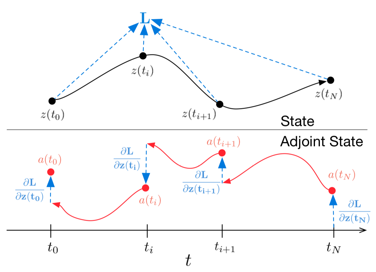
"Figure 1: Continuous backpropagation of the gradient requires solving the augmented ODE backwards in time.
Arrows represent adjusting backpropagated gradients with gradients from observations.
\n",
"Figure from the original paper
 \n",
"
\n",
" "
]
},
{
"cell_type": "code",
"execution_count": null,
"metadata": {},
"outputs": [],
"source": [
"def norm(dim):\n",
" return nn.BatchNorm2d(dim)\n",
"\n",
"def conv3x3(in_feats, out_feats, stride=1):\n",
" return nn.Conv2d(in_feats, out_feats, kernel_size=3, stride=stride, padding=1, bias=False)\n",
"\n",
"def add_time(in_tensor, t):\n",
" bs, c, w, h = in_tensor.shape\n",
" return torch.cat((in_tensor, t.expand(bs, 1, w, h)), dim=1)"
]
},
{
"cell_type": "code",
"execution_count": null,
"metadata": {},
"outputs": [],
"source": [
"class ConvODEF(ODEF):\n",
" def __init__(self, dim):\n",
" super(ConvODEF, self).__init__()\n",
" self.conv1 = conv3x3(dim + 1, dim)\n",
" self.norm1 = norm(dim)\n",
" self.conv2 = conv3x3(dim + 1, dim)\n",
" self.norm2 = norm(dim)\n",
"\n",
" def forward(self, x, t):\n",
" xt = add_time(x, t)\n",
" h = self.norm1(torch.relu(self.conv1(xt)))\n",
" ht = add_time(h, t)\n",
" dxdt = self.norm2(torch.relu(self.conv2(ht)))\n",
" return dxdt"
]
},
{
"cell_type": "code",
"execution_count": null,
"metadata": {},
"outputs": [],
"source": [
"class ContinuousNeuralMNISTClassifier(nn.Module):\n",
" def __init__(self, ode):\n",
" super(ContinuousNeuralMNISTClassifier, self).__init__()\n",
" self.downsampling = nn.Sequential(\n",
" nn.Conv2d(1, 64, 3, 1),\n",
" norm(64),\n",
" nn.ReLU(inplace=True),\n",
" nn.Conv2d(64, 64, 4, 2, 1),\n",
" norm(64),\n",
" nn.ReLU(inplace=True),\n",
" nn.Conv2d(64, 64, 4, 2, 1),\n",
" )\n",
" self.feature = ode\n",
" self.norm = norm(64)\n",
" self.avg_pool = nn.AdaptiveAvgPool2d((1, 1))\n",
" self.fc = nn.Linear(64, 10)\n",
"\n",
" def forward(self, x):\n",
" x = self.downsampling(x)\n",
" x = self.feature(x)\n",
" x = self.norm(x)\n",
" x = self.avg_pool(x)\n",
" shape = torch.prod(torch.tensor(x.shape[1:])).item()\n",
" x = x.view(-1, shape)\n",
" out = self.fc(x)\n",
" return out"
]
},
{
"cell_type": "code",
"execution_count": null,
"metadata": {},
"outputs": [],
"source": [
"func = ConvODEF(64)\n",
"ode = NeuralODE(func)\n",
"model = ContinuousNeuralMNISTClassifier(ode)\n",
"if use_cuda:\n",
" model = model.cuda()"
]
},
{
"cell_type": "code",
"execution_count": null,
"metadata": {},
"outputs": [],
"source": [
"import torchvision\n",
"\n",
"img_std = 0.3081\n",
"img_mean = 0.1307\n",
"\n",
"\n",
"batch_size = 32\n",
"train_loader = torch.utils.data.DataLoader(\n",
" torchvision.datasets.MNIST(\"data/mnist\", train=True, download=True,\n",
" transform=torchvision.transforms.Compose([\n",
" torchvision.transforms.ToTensor(),\n",
" torchvision.transforms.Normalize((img_mean,), (img_std,))\n",
" ])\n",
" ),\n",
" batch_size=batch_size, shuffle=True\n",
")\n",
"\n",
"test_loader = torch.utils.data.DataLoader(\n",
" torchvision.datasets.MNIST(\"data/mnist\", train=False, download=True,\n",
" transform=torchvision.transforms.Compose([\n",
" torchvision.transforms.ToTensor(),\n",
" torchvision.transforms.Normalize((img_mean,), (img_std,))\n",
" ])\n",
" ),\n",
" batch_size=128, shuffle=True\n",
")"
]
},
{
"cell_type": "code",
"execution_count": null,
"metadata": {},
"outputs": [],
"source": [
"optimizer = torch.optim.Adam(model.parameters())"
]
},
{
"cell_type": "code",
"execution_count": null,
"metadata": {},
"outputs": [],
"source": [
"def train(epoch):\n",
" num_items = 0\n",
" train_losses = []\n",
"\n",
" model.train()\n",
" criterion = nn.CrossEntropyLoss()\n",
" print(f\"Training Epoch {epoch}...\")\n",
" for batch_idx, (data, target) in tqdm(enumerate(train_loader), total=len(train_loader)):\n",
" if use_cuda:\n",
" data = data.cuda()\n",
" target = target.cuda()\n",
" optimizer.zero_grad()\n",
" output = model(data)\n",
" loss = criterion(output, target) \n",
" loss.backward()\n",
" optimizer.step()\n",
"\n",
" train_losses += [loss.item()]\n",
" num_items += data.shape[0]\n",
" print('Train loss: {:.5f}'.format(np.mean(train_losses)))\n",
" return train_losses"
]
},
{
"cell_type": "code",
"execution_count": null,
"metadata": {},
"outputs": [],
"source": [
"def test():\n",
" accuracy = 0.0\n",
" num_items = 0\n",
"\n",
" model.eval()\n",
" criterion = nn.CrossEntropyLoss()\n",
" print(f\"Testing...\")\n",
" with torch.no_grad():\n",
" for batch_idx, (data, target) in tqdm(enumerate(test_loader), total=len(test_loader)):\n",
" if use_cuda:\n",
" data = data.cuda()\n",
" target = target.cuda()\n",
" output = model(data)\n",
" accuracy += torch.sum(torch.argmax(output, dim=1) == target).item()\n",
" num_items += data.shape[0]\n",
" accuracy = accuracy * 100 / num_items\n",
" print(\"Test Accuracy: {:.3f}%\".format(accuracy))"
]
},
{
"cell_type": "code",
"execution_count": null,
"metadata": {
"scrolled": true
},
"outputs": [],
"source": [
"n_epochs = 5\n",
"test()\n",
"train_losses = []\n",
"for epoch in range(1, n_epochs + 1):\n",
" train_losses += train(epoch)\n",
" test()"
]
},
{
"cell_type": "code",
"execution_count": null,
"metadata": {},
"outputs": [],
"source": [
"import pandas as pd\n",
"\n",
"plt.figure(figsize=(9, 5))\n",
"history = pd.DataFrame({\"loss\": train_losses})\n",
"history[\"cum_data\"] = history.index * batch_size\n",
"history[\"smooth_loss\"] = history.loss.ewm(halflife=10).mean()\n",
"history.plot(x=\"cum_data\", y=\"smooth_loss\", figsize=(12, 5), title=\"train error\")"
]
},
{
"cell_type": "markdown",
"metadata": {},
"source": [
"```\n",
"Testing...\n",
"100% 79/79 [00:01<00:00, 45.69it/s]\n",
"Test Accuracy: 9.740%\n",
"\n",
"Training Epoch 1...\n",
"100% 1875/1875 [01:15<00:00, 24.69it/s]\n",
"Train loss: 0.20137\n",
"Testing...\n",
"100% 79/79 [00:01<00:00, 46.64it/s]\n",
"Test Accuracy: 98.680%\n",
"\n",
"Training Epoch 2...\n",
"100% 1875/1875 [01:17<00:00, 24.32it/s]\n",
"Train loss: 0.05059\n",
"Testing...\n",
"100% 79/79 [00:01<00:00, 46.11it/s]\n",
"Test Accuracy: 97.760%\n",
"\n",
"Training Epoch 3...\n",
"100% 1875/1875 [01:16<00:00, 24.63it/s]\n",
"Train loss: 0.03808\n",
"Testing...\n",
"100% 79/79 [00:01<00:00, 45.65it/s]\n",
"Test Accuracy: 99.000%\n",
"\n",
"Training Epoch 4...\n",
"100% 1875/1875 [01:17<00:00, 24.28it/s]\n",
"Train loss: 0.02894\n",
"Testing...\n",
"100% 79/79 [00:01<00:00, 45.42it/s]\n",
"Test Accuracy: 99.130%\n",
"\n",
"Training Epoch 5...\n",
"100% 1875/1875 [01:16<00:00, 24.67it/s]\n",
"Train loss: 0.02424\n",
"Testing...\n",
"100% 79/79 [00:01<00:00, 45.89it/s]\n",
"Test Accuracy: 99.170%\n",
"```\n",
"\n",
"\n",
"\n",
"After a very rough training procedure of only 5 epochs and 6 minutes of training the model already has test error of less than 1%. Which shows that Neural ODE architecture fits very good as a component in more conventional nets."
]
},
{
"cell_type": "markdown",
"metadata": {},
"source": [
"In their paper, authors also compare this classifier to simple 1-layer MLP, to ResNet with alike architecture, and to same ODE architecture, but in which gradients propagated directly through ODESolve (without adjoint gradient method) (RK-Net).\n",
"\n",
"
"
]
},
{
"cell_type": "code",
"execution_count": null,
"metadata": {},
"outputs": [],
"source": [
"def norm(dim):\n",
" return nn.BatchNorm2d(dim)\n",
"\n",
"def conv3x3(in_feats, out_feats, stride=1):\n",
" return nn.Conv2d(in_feats, out_feats, kernel_size=3, stride=stride, padding=1, bias=False)\n",
"\n",
"def add_time(in_tensor, t):\n",
" bs, c, w, h = in_tensor.shape\n",
" return torch.cat((in_tensor, t.expand(bs, 1, w, h)), dim=1)"
]
},
{
"cell_type": "code",
"execution_count": null,
"metadata": {},
"outputs": [],
"source": [
"class ConvODEF(ODEF):\n",
" def __init__(self, dim):\n",
" super(ConvODEF, self).__init__()\n",
" self.conv1 = conv3x3(dim + 1, dim)\n",
" self.norm1 = norm(dim)\n",
" self.conv2 = conv3x3(dim + 1, dim)\n",
" self.norm2 = norm(dim)\n",
"\n",
" def forward(self, x, t):\n",
" xt = add_time(x, t)\n",
" h = self.norm1(torch.relu(self.conv1(xt)))\n",
" ht = add_time(h, t)\n",
" dxdt = self.norm2(torch.relu(self.conv2(ht)))\n",
" return dxdt"
]
},
{
"cell_type": "code",
"execution_count": null,
"metadata": {},
"outputs": [],
"source": [
"class ContinuousNeuralMNISTClassifier(nn.Module):\n",
" def __init__(self, ode):\n",
" super(ContinuousNeuralMNISTClassifier, self).__init__()\n",
" self.downsampling = nn.Sequential(\n",
" nn.Conv2d(1, 64, 3, 1),\n",
" norm(64),\n",
" nn.ReLU(inplace=True),\n",
" nn.Conv2d(64, 64, 4, 2, 1),\n",
" norm(64),\n",
" nn.ReLU(inplace=True),\n",
" nn.Conv2d(64, 64, 4, 2, 1),\n",
" )\n",
" self.feature = ode\n",
" self.norm = norm(64)\n",
" self.avg_pool = nn.AdaptiveAvgPool2d((1, 1))\n",
" self.fc = nn.Linear(64, 10)\n",
"\n",
" def forward(self, x):\n",
" x = self.downsampling(x)\n",
" x = self.feature(x)\n",
" x = self.norm(x)\n",
" x = self.avg_pool(x)\n",
" shape = torch.prod(torch.tensor(x.shape[1:])).item()\n",
" x = x.view(-1, shape)\n",
" out = self.fc(x)\n",
" return out"
]
},
{
"cell_type": "code",
"execution_count": null,
"metadata": {},
"outputs": [],
"source": [
"func = ConvODEF(64)\n",
"ode = NeuralODE(func)\n",
"model = ContinuousNeuralMNISTClassifier(ode)\n",
"if use_cuda:\n",
" model = model.cuda()"
]
},
{
"cell_type": "code",
"execution_count": null,
"metadata": {},
"outputs": [],
"source": [
"import torchvision\n",
"\n",
"img_std = 0.3081\n",
"img_mean = 0.1307\n",
"\n",
"\n",
"batch_size = 32\n",
"train_loader = torch.utils.data.DataLoader(\n",
" torchvision.datasets.MNIST(\"data/mnist\", train=True, download=True,\n",
" transform=torchvision.transforms.Compose([\n",
" torchvision.transforms.ToTensor(),\n",
" torchvision.transforms.Normalize((img_mean,), (img_std,))\n",
" ])\n",
" ),\n",
" batch_size=batch_size, shuffle=True\n",
")\n",
"\n",
"test_loader = torch.utils.data.DataLoader(\n",
" torchvision.datasets.MNIST(\"data/mnist\", train=False, download=True,\n",
" transform=torchvision.transforms.Compose([\n",
" torchvision.transforms.ToTensor(),\n",
" torchvision.transforms.Normalize((img_mean,), (img_std,))\n",
" ])\n",
" ),\n",
" batch_size=128, shuffle=True\n",
")"
]
},
{
"cell_type": "code",
"execution_count": null,
"metadata": {},
"outputs": [],
"source": [
"optimizer = torch.optim.Adam(model.parameters())"
]
},
{
"cell_type": "code",
"execution_count": null,
"metadata": {},
"outputs": [],
"source": [
"def train(epoch):\n",
" num_items = 0\n",
" train_losses = []\n",
"\n",
" model.train()\n",
" criterion = nn.CrossEntropyLoss()\n",
" print(f\"Training Epoch {epoch}...\")\n",
" for batch_idx, (data, target) in tqdm(enumerate(train_loader), total=len(train_loader)):\n",
" if use_cuda:\n",
" data = data.cuda()\n",
" target = target.cuda()\n",
" optimizer.zero_grad()\n",
" output = model(data)\n",
" loss = criterion(output, target) \n",
" loss.backward()\n",
" optimizer.step()\n",
"\n",
" train_losses += [loss.item()]\n",
" num_items += data.shape[0]\n",
" print('Train loss: {:.5f}'.format(np.mean(train_losses)))\n",
" return train_losses"
]
},
{
"cell_type": "code",
"execution_count": null,
"metadata": {},
"outputs": [],
"source": [
"def test():\n",
" accuracy = 0.0\n",
" num_items = 0\n",
"\n",
" model.eval()\n",
" criterion = nn.CrossEntropyLoss()\n",
" print(f\"Testing...\")\n",
" with torch.no_grad():\n",
" for batch_idx, (data, target) in tqdm(enumerate(test_loader), total=len(test_loader)):\n",
" if use_cuda:\n",
" data = data.cuda()\n",
" target = target.cuda()\n",
" output = model(data)\n",
" accuracy += torch.sum(torch.argmax(output, dim=1) == target).item()\n",
" num_items += data.shape[0]\n",
" accuracy = accuracy * 100 / num_items\n",
" print(\"Test Accuracy: {:.3f}%\".format(accuracy))"
]
},
{
"cell_type": "code",
"execution_count": null,
"metadata": {
"scrolled": true
},
"outputs": [],
"source": [
"n_epochs = 5\n",
"test()\n",
"train_losses = []\n",
"for epoch in range(1, n_epochs + 1):\n",
" train_losses += train(epoch)\n",
" test()"
]
},
{
"cell_type": "code",
"execution_count": null,
"metadata": {},
"outputs": [],
"source": [
"import pandas as pd\n",
"\n",
"plt.figure(figsize=(9, 5))\n",
"history = pd.DataFrame({\"loss\": train_losses})\n",
"history[\"cum_data\"] = history.index * batch_size\n",
"history[\"smooth_loss\"] = history.loss.ewm(halflife=10).mean()\n",
"history.plot(x=\"cum_data\", y=\"smooth_loss\", figsize=(12, 5), title=\"train error\")"
]
},
{
"cell_type": "markdown",
"metadata": {},
"source": [
"```\n",
"Testing...\n",
"100% 79/79 [00:01<00:00, 45.69it/s]\n",
"Test Accuracy: 9.740%\n",
"\n",
"Training Epoch 1...\n",
"100% 1875/1875 [01:15<00:00, 24.69it/s]\n",
"Train loss: 0.20137\n",
"Testing...\n",
"100% 79/79 [00:01<00:00, 46.64it/s]\n",
"Test Accuracy: 98.680%\n",
"\n",
"Training Epoch 2...\n",
"100% 1875/1875 [01:17<00:00, 24.32it/s]\n",
"Train loss: 0.05059\n",
"Testing...\n",
"100% 79/79 [00:01<00:00, 46.11it/s]\n",
"Test Accuracy: 97.760%\n",
"\n",
"Training Epoch 3...\n",
"100% 1875/1875 [01:16<00:00, 24.63it/s]\n",
"Train loss: 0.03808\n",
"Testing...\n",
"100% 79/79 [00:01<00:00, 45.65it/s]\n",
"Test Accuracy: 99.000%\n",
"\n",
"Training Epoch 4...\n",
"100% 1875/1875 [01:17<00:00, 24.28it/s]\n",
"Train loss: 0.02894\n",
"Testing...\n",
"100% 79/79 [00:01<00:00, 45.42it/s]\n",
"Test Accuracy: 99.130%\n",
"\n",
"Training Epoch 5...\n",
"100% 1875/1875 [01:16<00:00, 24.67it/s]\n",
"Train loss: 0.02424\n",
"Testing...\n",
"100% 79/79 [00:01<00:00, 45.89it/s]\n",
"Test Accuracy: 99.170%\n",
"```\n",
"\n",
"\n",
"\n",
"After a very rough training procedure of only 5 epochs and 6 minutes of training the model already has test error of less than 1%. Which shows that Neural ODE architecture fits very good as a component in more conventional nets."
]
},
{
"cell_type": "markdown",
"metadata": {},
"source": [
"In their paper, authors also compare this classifier to simple 1-layer MLP, to ResNet with alike architecture, and to same ODE architecture, but in which gradients propagated directly through ODESolve (without adjoint gradient method) (RK-Net).\n",
"\n",
"