{
"cells": [
{
"cell_type": "markdown",
"metadata": {},
"source": [
"# Molecular dynamics simulations\n",
"\n",
"Classical molecular dynamics simulations involve numerically integrating Newton's equations of motion for $N$ particles interacting through a pair potential $V(\\mathbf{r}_1,\\mathbf{r}_2)$:\n",
"$$\n",
"m_i \\ddot{\\mathbf{r}}_i = - \\sum_{j \\neq i} \\nabla_i V(\\mathbf{r}_i,\\mathbf{r}_j)~.\n",
"$$\n",
"\n",
"If the system is sufficiently large, one can use MD simulations to study its macroscopic (thermodynamic) properties such as the dependence of the pressure on temperature and density -- the equation of state.\n",
"\n",
"In many case the pair potential depends only on the distance $r_{ij} = |\\mathbf{r}_i - \\mathbf{r}_j|$.\n",
"In this case the equations of motion read\n",
"$$\n",
"m_i \\ddot{\\mathbf{r}}_i = - \\sum_{j \\neq i} \\frac{d V(r_{ij})}{d r_{ij}} \\, \\frac{\\mathbf{r}_i - \\mathbf{r}_j}{r_{ij}}~.\n",
"$$"
]
},
{
"cell_type": "markdown",
"metadata": {},
"source": [
"## Lennard-Jones fluid\n",
"\n",
"Lennard-Jones fluid corresponds to a pair potential\n",
"$$\n",
"V_{LJ}(r) = 4 \\varepsilon \\left[ (\\sigma/r)^{12} - (\\sigma/r)^6 \\right].\n",
"$$\n",
"\n",
"The Lennard-Jones system has a rich phase diagram containing various phases (gas, liquid, solid) and the associated phase transitions.\n",
"\n",
"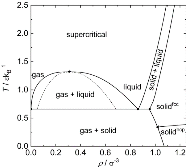\n",
"\n",
"To evaluate the properties of the LJ fluid, one would run molecular dynamics simulations for sufficiently long time to let the system equilibrate, and calculate its macroscopic properties like pressure as time average. The simulations are typically performed in a box with periodic boundary conditions to minimize finite-size effects."
]
},
{
"cell_type": "markdown",
"metadata": {},
"source": [
"## Velocity Verlet method\n",
"\n",
"For long molecular dynamics simulations it makes sense to use stable, time-reversal numerical schemes that conserve energy. The leapfrog method is a good choice. When applied to Newton's equations of motion it is know as Verlet method.\n",
"\n",
"Suppose we are solving Newton's equations of motion\n",
"$$\n",
"\\frac{d^2 x}{dt^2} = f(x,t).\n",
"$$\n",
"These are rewritten as\n",
"\\begin{align*}\n",
"\\frac{dx}{dt} &= v, \\\\\n",
"\\frac{dv}{dt} &= f(x,t).\n",
"\\end{align*}\n",
"\n",
"If we apply the leapfrog scheme to this system of equations, it will look like\n",
"\\begin{align*}\n",
"x(t+h) & = x(t) + h v(t + h/2), \\\\\n",
"v(t+3h/2) &= v(t+h/2) + h f[x(t+h), t+h)],\n",
"\\end{align*}\n",
"i.e. the coordinates are evaluated are full steps using velocity estimates at half-steps,\n",
"and vice versa.\n",
"\n",
"This is the essence of the Verlet method.\n",
"It's feature is that we do not need to keep track of coordinates at half-steps (only the velocities) and of velocities at full steps. In case we are interested in velocity values also at full step, these can be estimated as $v(t+h) = v(t+h/2) + (h/2) f[x(t+h),t+h]$.\n",
"\n",
"The full algorithm is as follows. Given initial values $x(t)$ and $v(t)$ one first computes\n",
"$$\n",
"v(t+h/2) = v(t) + \\frac{h}{2} f[x(t),t].\n",
"$$\n",
"Then each step of the Verlet algorithm corresponds to\n",
"\\begin{align*}\n",
"v(t+h/2) & = v(t) + \\frac{h}{2} f[x(t),t],\\\\\n",
"x(t+h) & = x(t) + h v(t+h/2), \\\\\n",
"v(t+h) & = v(t+h/2) + \\frac{h}{2} f[x(t+h),t+h)].\n",
"\\end{align*}\n",
"\n",
"The algorithm is straightforwardly generalizable to more than one variable."
]
},
{
"cell_type": "markdown",
"metadata": {},
"source": [
"Let us first write a code for integrating Newton's equations of motion for arbitrary central potential"
]
},
{
"cell_type": "code",
"execution_count": 1,
"metadata": {},
"outputs": [],
"source": [
"import numpy as np\n",
"\n",
"# Simulation parameters (can be changed later)\n",
"n_particles = 125 # Number of particles\n",
"density = 0.8 # Density of the fluid\n",
"box_length = (n_particles/density)**(1/3.) # Length of simulation box (determined by the number of particles and density)\n",
"temperature0 = 1.0 # Initial (desired) temperature of the system\n",
"time_step = 0.004 # Time step for the simulation\n",
"num_steps = 1000 # Number of simulation steps\n",
"\n",
"\n",
"# Initialization\n",
"# Initial position at the nodes of the cube\n",
"# Helps to avoid particle overlap\n",
"def initial_positions():\n",
" ret = np.zeros((n_particles,3))\n",
" Nsingle = np.ceil(n_particles**(1/3.))\n",
" dL = box_length / Nsingle\n",
" for i in range(n_particles):\n",
" ix = i % Nsingle\n",
" iy = (np.trunc(i / Nsingle)) % Nsingle\n",
" iz = np.trunc(i / (Nsingle * Nsingle))\n",
" ret[i][0] = (ix + 0.5) * dL;\n",
" ret[i][1] = (iy + 0.5) * dL;\n",
" ret[i][2] = (iz + 0.5) * dL;\n",
" return ret\n",
"\n",
"# Computes forces for a given vector of positions, interaction potential and its gradient\n",
"# Return a tuple: positions, total potential energy, and the virial part of the pressure\n",
"def compute_forces(forces, positions, potential, potential_gradient):\n",
" # forces = np.zeros_like(positions)\n",
" forces.fill(0.)\n",
" potential_energy = 0.0\n",
" virial = 0.0\n",
" for i in range(n_particles):\n",
" for j in range(i+1, n_particles):\n",
" # Vector of relative distance\n",
" r_ij = positions[i] - positions[j]\n",
" # Periodic boundary conditions (minimum-image convention)\n",
" r_ij = r_ij - box_length*np.round(r_ij/box_length)\n",
" \n",
" r_sq = np.sum(r_ij**2)\n",
" f_ij = -potential_gradient(r_sq) * r_ij\n",
" \n",
" forces[i] += f_ij\n",
" forces[j] -= f_ij\n",
" potential_energy += potential(r_sq)\n",
" virial += np.dot(f_ij, r_ij)\n",
" \n",
" virial = virial/(3.0*box_length**3)\n",
" return forces, potential_energy, virial\n",
"\n",
"\n",
"# Compute the kinetic temperature from velocities (kinetic energy) \n",
"def compute_kinetic_temperature(velocities):\n",
" return np.sum(velocities**2) / 3. / n_particles\n",
"\n",
"# Renormalize the velocities to match the desired kinetic temperature \n",
"def renormalize_velocities(velocities, temperature = temperature0):\n",
" Tkin = compute_kinetic_temperature(velocities)\n",
" factor = np.sqrt(temperature / Tkin)\n",
" velocities *= factor\n",
"\n",
"\n",
"# Apply the velocity verlet time step\n",
"# Returns the tuple of new positions, velocities, accelerations (forces), potential energy and pressure\n",
"def velocity_verlet(positions, velocities, accelerations, \n",
" time_step, potential, potential_gradient):\n",
" # Update positions\n",
" positions += velocities*time_step + 0.5*accelerations*time_step**2\n",
" positions = positions - box_length*np.floor(positions/box_length)\n",
" # Update velocities\n",
" velocities_half = velocities + 0.5*accelerations*time_step\n",
" # Compute new forces and potential energy\n",
" accelerations, potential_energy, pressure = compute_forces(accelerations, positions, potential, potential_gradient)\n",
" # Update velocities using new accelerations\n",
" velocities = velocities_half + 0.5*accelerations*time_step\n",
" # Add ideal gas contribution to the pressure\n",
" kinetic_temperature = compute_kinetic_temperature(velocities)\n",
" pressure += density * kinetic_temperature\n",
" return positions, velocities, accelerations, potential_energy, pressure\n"
]
},
{
"cell_type": "markdown",
"metadata": {},
"source": [
"Now the Lennard-Jones potential properties"
]
},
{
"cell_type": "code",
"execution_count": 2,
"metadata": {},
"outputs": [],
"source": [
"# Lennard-Jones potential as a function of squared distance\n",
"def lj_potential(r_sq):\n",
" r6 = r_sq**3\n",
" r12 = r6**2\n",
" return 4.0*(1./r12 - 1./r6)\n",
"\n",
"# The grandient term dV/dr / r in the rhs of Newton's equations\n",
"# for the LJ potential\n",
"def lj_potential_gradient(r_sq):\n",
" r6 = r_sq**3\n",
" r12 = r6**2\n",
" return -24.0*(2./r12 - 1./r6) / r_sq"
]
},
{
"cell_type": "markdown",
"metadata": {},
"source": [
"Perform the simulation"
]
},
{
"cell_type": "code",
"execution_count": 3,
"metadata": {},
"outputs": [
{
"data": {
"text/html": [
""
],
"text/plain": [
""
]
},
"metadata": {},
"output_type": "display_data"
},
{
"data": {
"application/javascript": [
"if (typeof Jupyter !== \"undefined\") { window.__context = { glowscript_container: $(\"#glowscript\").removeAttr(\"id\")};}else{ element.textContent = ' ';}"
],
"text/plain": [
""
]
},
"metadata": {},
"output_type": "display_data"
},
{
"name": "stdout",
"output_type": "stream",
"text": [
"1.4999999999999996 -0.15894785673871592 1.3410521432612836 1.0 -0.3154156116256416\n",
"1.5001135533336805 -0.1590917750637127 1.3410217782699678 1.0000757022224536 0.6843276016121962\n",
"1.9383068337180485 -0.5977073754917217 1.3405994582263268 1.2922045558120323 0.7051615207876363\n",
"2.001303243844825 -0.6601457213970912 1.3411575224477337 1.3342021625632166 0.6643988465099847\n",
"2.028619508086644 -0.6877169676321272 1.3409025404545165 1.3524130053910959 0.7694079884507117\n",
"1.9625004221886004 -0.6218942259413274 1.340606196247273 1.3083336147924003 0.5184337154741412\n",
"2.093669843537617 -0.7534163353646498 1.340253508172967 1.3957798956917447 0.826967832170502\n",
"2.030567541137616 -0.6895310805794714 1.3410364605581446 1.353711694091744 0.5751674922684135\n",
"2.168668336204985 -0.8277080837580238 1.340960252446961 1.4457788908033233 0.6902707035004116\n",
"2.081502536476681 -0.7410053478455663 1.3404971886311146 1.3876683576511206 0.7766335823289227\n",
"2.1043544365334927 -0.7640468899971166 1.3403075465363763 1.402902957688995 0.43664312260492566\n"
]
},
{
"data": {
"image/png": "iVBORw0KGgoAAAANSUhEUgAAAlEAAAHPCAYAAABz+I9wAAAAOnRFWHRTb2Z0d2FyZQBNYXRwbG90bGliIHZlcnNpb24zLjEwLjAsIGh0dHBzOi8vbWF0cGxvdGxpYi5vcmcvlHJYcgAAAAlwSFlzAAAPYQAAD2EBqD+naQAApF1JREFUeJzs3XdcE/f/B/BXwt4qiAIqS0WtWtDWvVDrnl+1dilurVq3tdZW3LbVWrVqnVVbW1e1rqrFgRv3aOsWQXGBouyZ5PP74/O7XI4ECCGQAO/n43GPJHef3H3uCLl3PlPGGGMghBBCCCEFIjd1BgghhBBCSiIKogghhBBCDEBBFCGEEEKIASiIIoQQQggxAAVRhBBCCCEGoCCKEEIIIcQAFEQRQgghhBiAgihCCCGEEANQEEUIIYQQYgAKogghhBBCDEBBFCGEEEKIASiIIqQEWrlyJd566y3Y29tDJpNh6dKliI6Ohkwmw6BBgwq1b0P34+PjAx8fn0IdmxBCShIKoggpAjKZDDKZzOhpAWDHjh0YO3YsbGxsMH78eISGhqJJkyaGZtWsVKxYUX099FnWr19v6izn6Y8//sBnn32Gli1bwtnZGTKZDJ988onB+3vy5AmGDBkCT09P2NjYwMfHBxMmTMCbN2+MmOuSw1jXw9h/J1J2WJo6A4SQgtm3bx8A4MCBA/D09FSvj46ONsr+vby8cPv2bbi4uBhlf/pKTU3FmDFjJOsUCgXmz58Pa2trTJ8+Xes9HTp0KK7sGWTevHm4ceMGHB0dUaVKFdy5c8fgfUVGRqJZs2aIi4tDz549UatWLVy8eBHLli3D4cOHcfbsWbi6uhox9+bNmNfDmH8nUsYwQojRAWD6/nsVJC1jjAUHB+tMHxUVxQCwkJAQvfdlTN7e3szb29uo+7x+/ToDwBo2bGjU/RaX48ePs3v37jGVSsXCw8MZAPbxxx8btK8OHTowAGz58uWS9RMnTmQA2MiRI42R5RLDmNfDmH8nUrZQdR4hJcSsWbMgk8kQHh4OAJJqrdycOHECMpkMs2bN0rldVzumvNpEMcawYsUKvPXWW7C1tYWXlxfGjBmDxMREQ08rT5cvXwYANGzYsEj2X9SCg4NRo0aNAlXX6hIZGYmwsDD4+vpqldbNnj0bDg4O+OWXX5CSklKo4+R04sQJdRWXpaUlfHx8sGDBAjDGjHqcgjL29TDW34mUPVSdR0gJ0aZNGwDApk2b8OjRI4SGhhZ7HiZMmIDly5fDw8MDI0aMgJWVFfbu3YuLFy8iKysL1tbWRj3elStXAADvvPOOUfdb0giBc4cOHSCXS3/7Ojk5oXnz5ggLC8OFCxfQrl07oxzziy++wLfffou3334bo0aNQnJyMrZu3YoZM2ZAJpPprF4tLqa4HoToQkEUISVEmzZt0KZNG5w4cQKPHj3KtXSpqJw7dw7Lly+Hv78/Ll68iAoVKgAA5s+fj+DgYDx//hze3t5GPaYQRBVlSdTSpUuRkJCgd/rAwED06tWryPKjy927dwEANWrU0Lm9Ro0aCAsLw71794wSNCxZsgTffvstPv/8c3zzzTfqEpqhQ4fi3XffxeLFi/HFF1/kW3JTVNe2uK8HIbmhIIoQopeNGzcCAGbMmKEOoADA1tYWCxcuRHBwsFGPp1Ao8M8//8Da2hp169Y16r41LV26FI8ePdI7fUhISLEHUUJ1aW6N/YX1BQlYcvPkyRPMnDkTzZo1w8KFCyWB0jvvvIPq1avjwYMHePbsGby8vPLcV1Fd2+K8HoTkhYIoQoherl69CgBo3bq11raWLVvC0tK4Xyc3b95ERkYGGjZsmGc14apVq7Bo0SI8f/4cb731FpYuXYqWLVvqfRxj9Wo0JaGNkjHa9Pz+++9ITU3FpEmTtKrKAMDBwQEAYGFhke++THVtjXk9CMkLNSwnhOhF+PVfqVIlrW0WFhZG716vT6Py7du3Y/z48fjyyy9x7do1NG/eHJ07d8bjx4+NmhdTE0pWcmvAn5SUJElXGPv374dcLkfnzp21tjHG8OzZMzg5Oen8HBSX4rwehOSFSqIIKcWEkgSFQqFze2Jiot43GiFdbGws/Pz8JNuUSiXi4+Pzrd4pCH0alS9ZsgSDBg3C8OHDAQDLly/HoUOH8NNPP2HhwoV6HacktIkKCAgAANy7d0/n9vv37wMAatasWajjZGdn49KlS3Bzc4O9vb3W9vPnz+Ply5fo2bOnXqU8RXVti+t6EJIfCqIIKcXKly8PAIiJidHa9uDBAyQkJOgdRDVo0ABXr17FyZMntYKo06dP5xqoGSq/RuVZWVm4cuUKpkyZIlnfoUMHnDt3Tu/jlIQ2UUJ7s7CwMKhUKkk1W3JyMs6ePQs7O7tCj1x/8+ZNZGZmIisrS+s4APDDDz8AgDpozU9RXdviuh6E5Ieq8wgpxWrVqgVnZ2fs3bsXcXFx6vXp6ekYN25cgfYljBs1f/58vH79Wr0+IyMj1+7ugwYNgkwmw6ZNmwp0LH0alb969QpKpVKrWqlSpUp48eKF3seKjo4GY0zvpaDnUlCRkZG4c+cOsrOz1ev8/f3RoUMHREdHY+XKlZL0oaGhSE1NxcCBA9XtlQQFvf5C4JqQkIDDhw9Ltq1cuRI7d+5Ely5d0LVrV732V1TX1tDroevaElIYVBJFSBHKaxLfVatW6awyMSYrKytMmjQJs2bNQlBQEHr37g2FQoEjR47A09NTMm1Mfpo3b47PPvsMP/74I+rWrYu+ffuqx4kqX748PDw8tN6jUqkAoMCNzvVtVA5oNx5mjJlNg+I9e/Zgz549AKAO7CIiItSfCzc3NyxevFjynnbt2uHRo0eIioqSDIS6atUqNGvWDOPGjcOxY8dQu3ZtXLhwAeHh4ahZsybmz5+vdfyCXn+h80D37t3Rr18/fPTRR3Bzc8Pp06dx9uxZNGrUCL///ntBLkGRMeR65HZtDfk7EQKApn0hpCjg/6dyyWt58+YNUygUDACzsrLSe9+tW7cu0LQvKpWKffvtt8zPz49ZWVmxqlWrsqlTp7LU1FSdU7XkNX2MSqViP/74I6tVqxaztrZmHh4ebPTo0SwhIUHnvgIDA5mTkxN7/fq13ufHGGMbNmxgANiIESNyTZOZmcksLCzYjh07JOtHjx7NWrVqVaDjFZXQ0NA8PwO6psnx9vZmAFhUVJTWtsePH7NBgwaxypUrMysrK1atWjU2btw4Fh8fr/P4Bb3+jRs3ZtbW1iw1NZVNmzaNeXp6MmtraxYQEMAWLFjA0tPTC3L6Ra6g1yO3a2vI34kQxhiTMWbi8fsJKcOeP38OT09PeHl54cmTJ6bOjlElJCTA1dUVkydPxnfffVckx2jcuDHefvttrF27Vr2uZs2a6NOnj94Ny0urgl5/pVIJJycn1K5dW12tRwjJG1XnEWJCf/75JwCUygawp0+fVlcnFpVJkyZhwIABaNSoEZo3b441a9bg2bNnGDVqVJEds6Qo6PW/desW0tPT0aBBgyLOGSGlBwVRhJjAzJkzce/ePezcuROWlpZaPcxKg+7duyMjI6NIj9G/f3/Ex8dj3rx5eP78OerWrYuDBw8affqZkqig118ofQoKCiqqLBFS6lB1HiEmIJPJ4OTkhHfeeQdff/210adMIaSgPvvsM6xYsQIRERGlsmSUkKJAQRQhhBBCiAFonChCCCGEEANQEEUIIYQQYgBqWF6EVCqVerJOcxn8jxBCCCF5Y4whOTkZnp6eWtMfaaIgqgg9e/YMVatWNXU2CCGEEGKAmJgYVKlSJdftFEQVIScnJwD8j+Ds7Gzi3BBCCCFEH0lJSahatar6Pp4bCqKKkFCF5+zsTEEUIYQQUsLk1xSHGpYTQgghhBiAgihCCCGEEANQEEUIIYQQYgAKogghhBBCDEBBFCGEEEKIASiIIoQQQggxAAVRhBBCCCEGoCCKEEIIIcQAFEQRQgghhBiAgihCCCGEEANQEEUIIYQQYgAKogghhBBCDEBBFCGEELORng5cuQJkZJg6J4Tkj4IoQgghZuHePaBWLeCdd4C6dYGnT3WnO3IEGDQIuHy5WLNHiBYKogghhJhcejrQty/w+DF/HRkJjB2rne72baBrV2DzZuC994CXL/Pft0IBxMUZN7+EABREEUIIMQPr1gH//gu4uwNHjwIyGbBnD3DnjjTdvHlAdjZ/npAAzJyZ934TE4HatQFvb+Dq1aLIOSnLKIgihBBiUioVsHIlfz5rFtCuHdC9O3/9449iugcPgO3b+fMffuCPq1cDzZoBLVuK2zTt3cvfl5EB/PRTkZ0CKaMoiCKEEGJSR4/y9lDOzsCAAXzd+PH8cfNmXpoEALNnA0ol0KULMGEC8MknfH1EBHDmDPDxx7waUNPp0+LzM2f449mzPO20aUBycpGdFikDLE2dAUIIIWXPv/8CVaoA5csDy5bxdYMGAY6O/HlwMFCnDnDrFrBxI5CWBmzZwqv5QkN5mo0bgX79gNRUYOFCvs+NG3mVn0AziLp3j6dp1w7IzOTr7t8Hdu8u8tMlpRSVRBFCCClWK1YA9esDNWsCBw/yRSaTNiSXyYDPPuPPJ04EZszgz+fPBxo14s8tLYEePYAPP+RpACA8XNxHXBxw966YVqUCRo3iAZSvL2BhAfz5Jw+uCDEEBVGEEEKKjUIBzJ3Ln796xXvaAbxnXo0a0rRDh/JSI4CXUK1cCUyfrnu/rVrxx0uXxFImofqubl1esgUA587xx++/F9cdOFC4cyJlFwVRhBCih8xM8eZclJ4/50HGzZtFf6ziEhEBVK3KG3+fOqV7uIFp07TXWVkBYWHA9et86IPRo3M/hp8frxrMzubXLiUFOH6cb2vZEnj7bWn6Vq2Ajh3587NnDTotQiiIIoSQ/MTFAV5egKendpf78+eBzz/n4xcZQ0gI77bfvDkQGyvdtnkzMHw4EBVlnGMVpe+/Bz74gPeMGzMGePKElwwJveo6dADef58/HzYMaNhQ937kch4AlS+f9/FkMqBBA/58zhzAxUXs8delizSIeustwNWVD+oJ0NAHxHDUsJwQQvLx999AfDx//scfwFdf8ef//Qe0bg1kZfHu9XfuAHZ2hh8nNpaPxg3wHmn9+gEjR/JBJa9d4w2vAV6yc/0676m2di2vBuvUyfDjGtvjx8CUKfx5djbPu0CoOqtTB1iyhDcI9/U1znEbNACOHePDGggCA/m10Qx+W7QQtwFAdDS/3i4uxskHKTuoJIoQUqbExvJGyPv36/8ezeqeU6fE54sW8QAK4IGD5s1bH/v28UbWwj4uXZJuP32ad+Nv2FBalXXzJnDoEDBkCDBuHNC5Mw/uTE2pBNav5yVLgtx6vtWpw0uP/Pz4ozEIJVGCPXv4387SEggI4AN5ymTitSxXjq8DxKER9uwBNmwAGDNOnorLvn3AmjW8zRkpRowUmcTERAaAJSYmmjorpJRRKhlbsYKxw4dNnZOSp29fxgDGrK0Zi4rS7z2tW/P3AIy5ujKmUjGWns6YoyNf16YNfwwJ0T8ft24xJpfz940bx9fNnCnuZ+xYxmQy8bgAY7a2jA0cyJ+7u0u3vfNOwa5DUfjqK2meNJcqVaSvz5wx/vFjYsT9d+qkvf3hQ8bu3pWua9aMp9++nbErV8RrvmJF4fKiVDI2dChjDg6MNW7M2JgxjD15ojvtkyeMHTzI2MuXhh3r77/F854+Xf/3rVzJWJcujJ09yz/TSUmGHb800vf+TUFUEaIgihSVpUv5F6aFBWPXrpk6N+bh7FnGTp3KO41SyVi5cuINZ84cfvPYsIGxadMYS07W/T5PT2kA8OwZY0eP8ueenozt3cufv/WW/vkNDRX3Z23Nb6SdO0tv4AoFY9ev8+0AYwsW8CBAMy9duvDPAaB/UFgUlErGKlcW81W1qjSfw4dLX8fHF00+QkMZq16dsTt39EsvBKXz5zP2xRdi/po10/+YQlCtads27UCyUSOeVvDPP4w1bSpuL1+e/70L6r33pEG+Upn/ex49EgNGNzce6MnljC1eXPDjG2LrVsYGDeKBrTmiIMoMUBBFiopQ8gEwNnGiqXNjemvWiNdj6dLc0928Kb2p1a7Nv8yF16NGab8nJUXcXrEif/z7b8bmzePPP/iAB1UAvwnlDMTi43n+7t+Xru/eXZqXTz/lN0CAsQsXtPN99qz4esAA8Yb55AljzZvz12vXMpaRwdjnnzPWp0/RBNgvXvDzT0vjr7dt46Vi/frxPDg7M/bgAQ8qNEufVq+Wnq+5mDOH52fwYGkwIpMxlpoqTXvmDL+2t26J65KSGHv3XcYqVZKuF0ovQ0IY++knMRA+f55vz8pizMdHPJ6zM3/082PszRv985+aypilpfTaCvl49IiXDur6HAg/xHIudnaMvXrF01y5wljPnoytX69/foRz0wwWc9IshX3nnbzT5kb4/BUVCqLMAAVRpCgolYw5OYlfejVqmDpHppWcLN6AAMZcXHL/gl23jqcJCmLMxkb7BuLgoP3eGzf4tgoVxKrAxYsZ69aNP1+2jKfz8uKvT58W35uWxljNmmIA9uyZuM3bm6+fPVv7JpaZmfc5Z2Qwtm8fY7Gx/PWsWfy977/P2OTJ0qAvvxtyUhJjly7lf0zG+A3b11csWWKM51cz/x9/LKZv1Upcf+IEzx/Ag0Bz8fvvPE8tW/JASPNcrlwR0718KZZili8vBiZCECYETIwx9vy5WMrz+DFf97//8dfz5vHXu3aJf6OoKB5sC0FV9+76Bxbh4fw9Xl5iML15M39/UJD4uRbyIfjoI76tQweeV82q423b+PuFzy7Aj6OPTZt4tXPbtowlJOhOI/wAEZZLl/Tbt2DjRh44hoQYFoDpQ9/7NzUsJ6SEefpUOt/X/ft8bKGyaudOICkJ8PfnYxElJuY+eKLQQLxLF74I3N15l/fUVD62EGN8nCGAd9EHgOrVgXr1+PMbN/jQBgDQpAl/FLrLazYO//VXcTTsly+BL77gzxUKICaGPx82TBxQEgCaNgWsrfM+ZxsbPkGv0Ci6fXvxWqxYIaZ7+RJYtUr3Pp484aOAV60KvPsuX4Q56nKzaZM4vMLmzXwf6enSNMKwBQAfEkJQty6fLHjlSvOaCLh6df7477/ikBLC31lzrK4DB4CEBP78zRugbVtg61bpBMmXL/PHv/7in6F33uHXFwDatOGPwmCfBw/yx48/Bnx8gAoVgF27+N92/37dkynrIgwo2qKF2Nvw5k3ec1ToFZmayq+9posX+ePkyfz5P//wTgoA79Dw77/Skdy//JKfk4Ax3rty0iTxuqSm8jkNMzL4/1G3bmKvVk2anTM0r0VOCoX23IYKBc+zQsE/g8L/ockUTQxHGKOSKFI0IiL4r7dq1cRfmlu3mjpXpiM0DP7mG7EUZvBgXlJw9Kj0l6rwy/qvvxg7flysUtiwQWyzM2ECYx9+yJ/PmcP3K5Sw7N7NnwslgTY2YgnO3Ll83Ucf8dcqFW8jJVT5Cb+6z5zhpQIA/zWtUPDqLy8vXuVz7FjBr0FWlrR0MjCQ/1oHdLfT+vlnxqystEvivv4692OoVHy/mumFayNUZb79Ns+LQCgl8fcv+DkVl5cvtUsjP/2UP582TUz3ySd83dixjDVpIn2PcC3lcl762LOnWMooOH2ar6tShb+uXl38LGoSOhd07Khf/jt25Ol//JGx5cv58169eAmpZh5r1hTf8+qVuF6zbdrOnXxd/fpiPho1Eksbt20T0546Je5j9Gi+TihdA8ROF+3aaZcWCaWwwjVt146vz8gQPz9xcYwFBPBSraNHxfeePSs9ryFD9LtOBUXVeWZA+CM8e5bIUlKY1pKzIaKuNMKSs4qhIGlTU3NPm7POvyBp09LyzoehadPTjZdW8583I8N4aTUbbmZmGi+tQiE9t23beNCkmebXX/mXR9OmjI0fL1at5LXf7Gxxv1lZ+qfNzs47reYNsyBpFYq802pWLeWV9tIlfv4WFrwK5fBh8WYmVNetXMlvGkJ1ikzG2OvX/O8SHs57RaWk8CqQnEGFhQW/iQg3RKFqT1gaNeLvzcgQjy2T8TYwQjWPgwNjT5/yIAzgjXj//JM/9/YWz+XVK8YiI6XnV5DviC5dxHxt2MDbSgltZS5eFNNdvy6ub9GCsT/+4FUwAK/OSkrS/X8vXGsrK/GavPsuf2zVigcjOduDpaUxduQIP6a5fkcolfxGLVy7WrUY+/57/rxzZzFdnTp83YED/PM5aRL/fDg68qpVe3u+/do1sdrv4kXx/15oNwcw9t9/4vNHj6TfEcJnzNKSfyby+o5ISxODlXPnxA4OAQFig/lx48SqushI/ncSOkr4+0v/71+8EPMldBJYt05aRdy9O08/dqy4zsaGf8aFtnpjxvAfC0I7MKGxfHa2NGjdt08MuC5f5sGauzv/7GoG6DVrip9Lofpb6J1qb8//n/X9PlEq9UtbpoOoV69esXXr1rFevXoxf39/Zmtry5ydnVnz5s3Z+vXrmVKfrgsaYmJi2ODBg5mHhweztrZm3t7ebPz48ez169d5vk/4IwCJWl/OAP/S0yT8E+paWreWpnVzyz1tzq7OQtSva6lTR5pW+KLQtXh7S9O+807uad3cpGk1u4jnXOztpWk1bwa6Fk1CG5XcFs0v1JCQvNPGxYlpR4/OO61mL6gpU/JO+99/YlrNHlm6FuFLlzHx12xenwmhZCRnW46cy4ED4n6FEorclh07xLQ7duSdduNGMe2BA3mn1ewyLpRQ5LZ8952Y9uLFvNMC/Foxxtuw5Je2f3+eNioq/7T6LiEhjCUm5v0/rLnUqMEfW7TIO11BviMaNOBtajp35jervL4jAN4WRvjhUK1a7umE7wjh/0ez/VnOpaR+R2i2/clviY7m+83vO8LCggfXjBXsO0IoAcptuXiRsf37eW+6nMNG6Fq2buUlS/mlE74jAgLyTztqlNj+Sp/lq6/0+44QlgUL+Oc5rzRduvCAF+DDOuSVNjRUvL6aAayuZcoUnq5Mt4nauXMnhg8fjvPnz6Nx48aYMGEC+vTpg//++w/Dhg1Dv379wBjTa1+RkZFo2LAhNm7ciEaNGmHixInw8/PDsmXL0LRpU8TrqvAlJZ6pB6xjTLvdQE4VK/I5wQDt6UFyOnmSt48prYYP5482Nnmnq1GDj/CtD2FUa4APDJkfZ2feVkMf9+/zR6G9jDE4OfH2Sn/9xQeXzM+UKeIgl/kNdvnbb7z9CcDbjpU2+v4dHB2BatX0S+vvn//nUZf8/hb37wN9+gAXLvA2afmpVUucnFkfQtutvFy6xNtcAfrte+dO3sYqLU2/PBw5Ajx6lHeaatV4e8KgID5oqsnkGWKVUMeOHWN79uxhCs1yT8bY8+fPWdWqVRkAtnPnTr321aFDBwaALV++XLJ+4sSJDAAbOXJkru+l6jzD0ppDdV7XrvxXydChuVcBCOd1/Dgvks+rukCgWZ335Amv9jl+XLuo/vp16a+jnj3FNMIva6G0pm5d/X7dubjwkprSUp03aRI/r/r1xWusVPIu5NWq8eo7zfGdHB2lPdV0Fevfu8dLGA4d4p+t6dN5m5Nbt8Q0R48y5uHBS04SEvg6ocRB87OenKy9//v3pX+Tzz/P+zoU9jvi2TOxSuXMGca+/ZY/r1lT+nlPTRVLHT08pFV6Bw+K41BNmsTTHjokPY/vvivZ3xEjR4rnMmsW/9uVL89fR0TwNmQAr0IX5Pw+EXoeCqVDvXqJaYX/e81xqADeBk3Xd8S4cXx727a8alaornr5UqwtqFiRV6NZWPAhJ4R85Pw+SE3lA4kCvARU+Fvevq37/15ocwkw9ssv0jTC2GhCdbBMxsd5EtoWAnzsJyH9s2fStnc+PuL/7Qcf8DQTJ2p/V2m+54cf+GOdOuL/j0zG23IJ35cF+T6h6rxCmj9/PgPAxowZk2/aBw8eMADM19dXqwowKSmJOTg4MDs7O5acywh91LC8ZLp9W/oP/eCB7nSvXomNQx0cGNuyRf9jpKbyMYqEY+R8r9CeRrgBajYObtmSrxMaeY4ZoztoatCAf6F9/DFv+wAUbABBc6FS8cCmfHn+qFLxL2ehsevevbm/d9gw8XoMHVp8ec6NSiWONQXwxsBFrX9/fqzy5cXP0+rV2unS08XG6cKYVCoVbywO8Abzwteg5sjgAG+QXJItWSKey2+/8XVCh4WtW8XqohEjct/H1KnSa6Jr/DbNhtcAD1B12bJFmu6TT3iQ2bs3f+3uzoe3ePVKHNNJoFl9KVSvarbHAnh7p7yGBtiyRff3WXy8dD/VqvH1EyaIgd2jR9L3CHkWFiGImzOHbxfaBwKMNWwoDcg8PPgxhXVCQFWvXu55NxYKonKxaNEiBoBNmDAh37Tr1q3Ls7RJKKU6qtl1QAMFUaZ35w7/Mtu4Uf/xRDZskP7T5zaNwtdfawcu+vaSy/mF6+4u/bXUuDFfP2OG+MtsyBBp2xVhPKLbt/mXl48Pb1x98CBvc6R5vk+fir8ecw76aO5y3lA2bBDbozRtmvff9dw5/qvV2lo65o8ptWsnnkteAaCxREWJY1gBPAjXLG3UJDR+HziQvxZKJezspL24cjbGLug4P+ZG6BQAiG2ehg7lr2fO5CVCuQWfAuEGLyzC+GGaIiOlaXIbRynnqPSA2IDc2pqPuZUb4TsDkE59I7QfAqSlZAWl+SNAaKurUvHAO2dAxxj/ThoxQrvdpvAjULMx+6JF0ny2bcvTCG0HXVz447BhhudfXxRE6ZCdnc3q1q3LALDDekw6NmXKFAaALc5lHPwxY8YwAGzVqlU6twt/hJiYGJaYmKheMjTL/kmRefNGOg2F8MtHIPyqvneP/5IWqptGjeLphdIbGxvewyvnNBVCd+9ffhFv6tbW4ojEubl8WfxltXu3WOW0e7eYb2F7dLT0ZqW5aDZuVyrzHyxRGOW8sHOCFSfNYQJ0XYe8biaCiAj9pwApDkJVDSAOllnUUlJ4L7m//5ZWq+Z05oyYt88/F0vyhKBKk5+fmNbQOd/MhULBz/fPP8V1ixfzc+vRg5c0A4z9+2/u+xCqzPIKkFUqMUh499288/TJJ7zURvj8AzwYzu/W9csvYvq5c8X1whAc+QWD+RFKwgFe0q2vsDDp9dH8UXPyJGOrVvEqUmHke4CXsjPG2MKF0veuW2d4/vVFQZQOkydPZgBY586d9Uo/fPhwBoCty+Uv9uWXXzIAbMGCBTq3i73zpEuoZlcBUmS++077pnvsGG+LVKcO/0W1YoXYFb5XL/4lJ/Qo2rJF2vvF31/85ZiZKdbbR0XxL+Fevfjr2rWl3ZA1ZWWJwZfQS0y4qQoFnnv28NfCSOS6etbY2uZ+jNwIVYTCOEYlwZEjPM8ODvwXqzBaNqD/ODrm5uZNHmy/956pc6Kb0L0/v2BVs+ddUY0abUo5231VqZL3nHSaASjAhyrQ5coVXjITE5P38RUK3mNYpeIByMGD2m3kdImN5aPr5wxUkpN5W8/WrQs3ZYrmHIiavWjz8/q19PrkNtmxZsC0aRNfl3NokadPDc+/viiIyuGHH35gAFhAQAB7qefPpvyCqOnTpzMAbOHChTq3U0lU0crrCyU7W6z6+vlnseFoy5bS8U1yLn//LQZHDx/y7rCDBomNTIXB965e5a/LlxdvIK9fi19eu3bxarOGDXmjcOH/UPg1WKGCWAohjO1SuzZ/LYz9JMzjpvnLTFhydiXXh1BlUZKmiRG6sn/2GX994QJvFN20qVjtUhI9epT7TcQcrFsnloa2bq07SAoL493hP/+82LNXLJKTpVMDzZqVd/qcQ2bkVlVXHJ49k861aEyaQXZubbpyIzQpsLLKPY3mdXzxgq9TqcTvgoKUfhUGBVEali5dygCw2rVrs+fPn+v9PmNV51GbKONKT+d1/TIZ7+2ii1C0XrEiT6/ZJijn4usrBirCGCmurtIbhzAonJ0dH21a6K0THCw9rjAeTL9+vBpAOMakSbydknBj+uUX8T1Pn/J1FhY8r8HB/PXmzXy7ZluLDh3449ixBb9umoPcFWSC0+Jy8SKfqFeYX0749SmT8SpXUrwiIniDa3P8rBQXoZq+Vi3tgURzUiik3yul1ePH/PvRzk46tp4+wsP5963muHW6HDqkXW2ZlcXb3hW0BN5QFET9P6Ehed26dVlsARsgCA3LR+TSJYMalptGzsHocrZBysjgJUAATysQpvIA+IjCiYm8DcTr17yEQ3OfOauKVCpxqodKlcT2RTl74Fy+nHspl7DknDRTpRJLuq5fF9txCQNvJiXxEaI/+EDswm9ocbxQHXb0KO91OHo0D/gCAngpWWGqZa5f570VK1bMu8H006e8lE/TH3+I16d8eV4NIfy93n/f8DwRUhhKJe/AoW+pYVkIohjjDchz/g+XNhREMcYWLFjAALDAwEC9q/A0CUMc+Pj45DnEQUrOgUn+HwVRhvvvP35jL1eON+oWxMeL3bCFkiWh2osx3lZJGOPJwYH3DBGcPy9+wY0bJz2eSiUdX0Uz+BJERoojTQuLZomSsB9h2AOANx4VSpYA3r4p51g6jIndqdetE9MWxcdGGMtm4ULpEAvConmtC0KplLbdcnTU3ebjjz94iZuFhTgyukIhjqqvaz63a9cMPVtCitecObzktKDVXMT8lPkgas6cOQwAa9iwIYvP2a0qh6ysLHb79m32QMeAQMYYbJOCKP3ExPAqhLQ07WkYxo/nN12hOuvtt/kXFcB7rAglKEJ9vZ2ddNJKwdatvMeHro/E6tX8vXJ57tVHOds96Oqtozm1y7p1YulSw4a8KFwXodRFmO8q55QYxiI0thfG/gH4vFjChKuuruKv7n37eA+l/KoxGBMnBbW1FUu7xo+XpnnzRmwzBvCAVKXijf0BsZ2Y5uSuvXsb+QIQUoSUSl6yTUq+Mh1Ebdq0iQFgFhYWbMKECSw0NFRr2agx6VdUVBQDwLx1tNZ98OABc3d3ZwBYz5492RdffMGCg4MZAFazZk32StfAGP+PgijR7dv8xu3vz3tc5RQeLg4EKCyVK+seSFIu56N8p6WJDT+F0XeFMUzWri14HlUqXr137Fje6TTn7dI13k5yMu+e/PHH+Q87IJg2je9PGFYhKKjA2ddLzjnrWrbk67OzxcB13jzp2EydO4tBakgIL2XKeX2FkZg//ljsymxnJ+3CP2sWX1+tmtg27PZt8dyFbvQJCXw/Q4boDnYJIaSolekgKjQ0lOkaWkBzaa0xo29eQRRjjD1+/JgNGjSIVa5cmVlZWbFq1aqxcePG5VvCRUGUSHOAQUdH6ai2iYm6J0AVxmxZu5ZX9wQG8l52J09q73f5cnHWb3//vMfCKax//uFTipw6Zbx9rlwpPfcePYy3b02vXkmPo1mt+dtv0kBVM93x42KJkRDgagaQHTvy9atX84Dr3Xf5a2Gg0vh4caC8HTvENmUbNojjzmhOZkwIIaZUpoMoc0FBFPf8uXjzdXfnj927i9uFHjB+fryB95QpvCpJH0Lg1KoVr4oCxF5tJcn+/dKgRY9ZiQwm/A0APsCdQKEQ5+UCeNAqjAnTpYt0XCCAD/MgEAYMPXeOvxamcrC35wGiMPpz3bq8ykPoxThqlNjG7Z9/iu6cCSGkIPS9f8sLMXcxIWqxscDAgUDDhsDChUB2trjt6FH+2LAhcPIkn6V8/37gzh0gJgZYt45vX7cOaNQIWLQI6N5dv+O2b88fT50C4uP5jOUffWS88youOWeG13dWeUO89Zb4vHZt8bmFBbByJeDkBHh5AVu2AFOn8r/XwYPA5ct8Fnvh/deu8cf4eODZM/68bl3+2KMH0Lo1n7V9zBhgwwa+fv58QC7nnwUA+OMPIDmZz3Zfq1bRnTMhhBQFS1NngJR8WVlAp07A9ev89dWrPFj66y9+Y/7vP76+cWN+o+zRA9i7F1ixgm/PzuY33LZtC37soCDAwwN4/py/XrUKsCyBn+qcQVNRBlH16gHh4fx5kybSbW3aAC9f8sDJ2pqv69kT2LOHP58yBUhKAm7eFP/e//7LH319eQAG8EDpwAHgp5+AX3/lAfOECWJw/M47/PHVK/5Yty5gZWXc8ySEkKJWAm83xNysXs1vqG5uwLRpQGgo8PffvCQjJAS4fZunE0o9xo7lQdTKleI+vvrKsGPL5cDWrcCMGbwEKji4UKdiMuXK8VKelBT+uiiDqKlTgcOHgf79AVtb7e02NtLXK1bw6+zpCUyfDuzYwddv3QrcuAFERfHX9epJ3+foyI81dSqvAJTJxG3+/oCLC5CYyF8HBRnn3AghpDhREEUKJSMDmDuXP58/HxgxAlAo+M123TppECVU17RtC1SvDjx4wF83agS0a2d4Hlq3Bs6cMfz95kAmA3x8xFK7ogyiqlQB7t7VP72XF7Brl/g6MJA/vnrFq1EF9evnvg/NAEp43aCBWCLWqJH++SGEEHNBbaJIoezezW+mVasCQ4bwdQMG8MezZ4GnT4GHD/lroSRKLuftnuRyXoXz/ffaN9mySLMaMmcbKXNSqxb/2+WUsyQqP0KVHsCrEQkhpKShkihSKGvX8sdhw8QgwMsLqFMHuHWLt4dRKnlbGU9P8X29eomlIdWrF2uWzda33wIdOwLz5ukOUsyFpSWgUmmvf/fdgu1n5EjetiowEKhRwyhZI4SQYkVBFDHYnTu8AblcLpZCCZo140HUzz/z17VqaZc2UfAk1aEDkJAAODubOif5mzQJWLKENzq/excYPJg3LC8If3/e+YAQQkoqCqJIvrKzeWPwFy94yVOlSny9MDRBt268nY2mpk2B9euB+/f5a82u9CR3Li6mzoF+Zs3ijfg7d+Y9LAkhpCyiIIrka+dOsdquRg1g8WLe22r7dr5u2DDt9zRrJn1NYwCVLk5OPHgmhJCyzIxbXhBz8fvv4vPt23kAdeUKbzTu6MiroXKqWRMoX158XdBGx4QQQoi5oyCK5CkrCzhxQnz95AkQGQns28dfd+yoPa4QwNtJCV3hAaBVq6LMJSGEEFL8KIgieTp/HkhNBSpWBJo35+vCw/lgmQAffTw3S5fyUcq//LJkNJYmhBBCCoLaRBEtDx8CP/4IuLqKo1G3b8970509C2zaBPzzDy9t6to19/3Ur8+DMEIIIaQ0oiCKSCQn8xHAnzyRru/Xj09NMncucO4cX9eiBQ+0CCGEkLKIgigisWULD6Dc3PigmTdu8J523brxQTNtbIDMTJ62Tx/T5pUQQggxJWoTRST27+eP06YBV68C167xhuVWVnyyWmFQzYoVgYEDTZZNQgghxOSoJIqoKZXiRL7t2mn3sAOAH37gDcxbtODVe4QQQkhZRUEUUYuJ4W2irK15o3BdbGyAjz8u3nwRQggh5oiq84javXv80d+fpvIghBBC8kNBFFET5rmrUcO0+SCEEEJKAgqiiBoFUYQQQoj+KIgiahREEUIIIfqjIIqoURBFCCGE6I+CqDLs+HFgwgTg0SNAoRCneKEgihBCCMkfDXFQRt2+DXTsyIOn8+f5SOUKBR9Q08vL1LkjhBBCzB+VRJVRP/zAgyYAuHBBHKm8enU+yCYhhBBC8ka3yzJIqQT++IM/t7Lij4sX88eaNU2TJ0IIIaSkoSCqDLpyBXjzBnBxAb79lq979ow/1qtnunwRQgghJQkFUWXQkSP8sW1boGdP6TYKogghhBD9UBBVBh07xh/btwf8/IAqVcRtLVuaJk+EEEJISUNBVBmjUgGXL/PnLVrwx3XrgKpVgS++ANzdTZc3QgghpCShIQ7KmIcPgeRkwMYGqF2br+vUCXj82LT5IoQQQkoaKokqY65d44/16ok98wghhBBScFQSVUYkJgJZWWIQFRRk2vwQQgghJR0FUWXA338D//sfHx8qM5OvoyCKEEIIKRwKokq5xERg4EAgLU26vlUr0+SHEEIIKS2oTVQpN3cuEBcH+PjwHngAULkyUKeOSbNFCCGElHhUElWK3b0LLFvGn//0E+DpCfz4IzB2LCCTmTZvhBBCSElHQVQpxRgwaRKfZLhbNz6MAcDHhCKEEEJI4ZXK6rw//vgDn332GVq2bAlnZ2fIZDJ88sknBd6Pj48PZDKZzqVy5cpFkHPj2bwZOHiQD2Pw/femzg0hhBBS+hS6JColJQX3799HSkoKWprJnCHz5s3DjRs34OjoiCpVquDOnTsG78vFxQUTJkzQWu/o6FiIHBatmzeBMWP481mzgJo1TZodQgghpFQyOIh68uQJxo0bh/3790OlUkEmk0GhUAAAzpw5gxEjRmDVqlVo06aNsfKqtx9++AFVqlRB9erVcfLkSQQHBxu8r3LlymHWrFnGy1wRu3ePz4mXlsYnGJ42zdQ5IoQQQkong6rznj9/jsaNG2Pfvn3o3r07mjZtCsaYenvjxo0RFxeH7du3Gy2jBREcHIwaNWpAVsZaT+/ZAzRpArx4AdSvD+zYAVhYmDpXhBBCSOlkUEnU7NmzERcXh6NHj6JNmzaYPXs2IiIi1NutrKzQsmVLnD171mgZNZXMzExs2bIFjx8/hoODA+rXr49WrVrBwkyik4wMICwMWL4cOHaMr2vUCDhwAHB1NW3eCCGEkNLMoCDq4MGD6NGjR55VddWqVcPp06cNzZfZePHiBQYMGCBZ5+vri40bN6J169Z67SMpKUny2sbGBjY2NgbnaflyXur08iUfxiA7m6+3suI98ubMAaytDd49IYQQQvRgUHVebGwsatSokWcaKysrpKamGpQpczF48GAcO3YML168QGpqKv7991+MHDkS0dHR6Ny5M27cuKHXfqpWrQoXFxf1snDhwkLl6/59IDwc+O8/HkB5egITJ/L2UN98QwEUIYQQUhwMKomqUKECnjx5kmeae/fumf0wAPkJDQ2VvK5bty5Wr14NR0dHfP/995g1axb+/PPPfPcTExMDZ2dn9evClEIBwIABQNOmvLquZk0+GnkZa/5FCCGEmJxBJVHNmzfHvn37EBcXp3P7/fv3cfjw4UL1ijNno0aNAgCcOnVKr/TOzs6SpbBBVKNGwEcfAR07Ar6+FEARQgghpmBQEDV16lSkp6ejdevWOHz4MNL+f3bb1NRUHDp0CN27d4dcLsfkyZONmllz4e7uDgAlvrqSEEIIIYYzqDqvcePGWLt2LUaNGoWuXbuq1wtVVpaWlvj555/x1ltvGSeXZubChQsAAD8/PxPnhBBCCCGmYvBgm4MHD0aLFi2watUqnD9/HvHx8XBxcUGTJk0wduxYBAQEGDOfRSY7OxuRkZGwsrKCv7+/ev3Nmzfh4eGBChUqSNLHxMRg7NixAGDQVDKEEEIIKR1kTHOUzFJiz5492LNnDwA+RMHff/8NPz8/9bQ0bm5uWLx4MQAgOjoavr6+8Pb2RnR0tHofs2bNwjfffIPg4GD4+vrCyckJDx8+xIEDB5CRkYEuXbrgzz//hHUeXeGSkpLg4uKCxMREScNyQgghhJgvfe/fhZ47zxxdv34dmzdvlqx7+PAhHj58CADw9vZWB1G5CQ4Oxt27d3Ht2jVEREQgNTUV5cqVQ4sWLTBgwAAMGDCgzI2ITgghhBCRXiVRjx8/NvgA1apVM/i9JR2VRBFCCCElj1FLonx8fAwqddGclJgQQgghpDTRK4gaOHAgVV0RQgghhGjQK4jatGlTEWeDEEIIIaRkMWiwTUIIIYSQss6gIOrly5c4deoUkpKSdG5PSkrCqVOn8OrVq0JljhBCCCHEXBkURM2bNw/dunWDhYWFzu0WFhbo3r07Fi5cWKjMEUIIIYSYK4OCqCNHjuC9996Dg4ODzu0ODg7o0KED/v7770JljhBCCCHEXBk02GZMTAy6d++eZxo/Pz+EhYUZlCmSt61bt+LkyZMA+DASQs/JnM91rUtKSoKFhQXKly8PS0tLyGQypKenIzU1FUqlEo6OjrC3t4dSqUR2djaysrKgVCphb28PBwcHKBQKpKWlQaFQwMLCAhYWFmCMSRaVSoXs7GxkZ2dDoVDA1tYWFStWVA95oblNpVKp9yMsKpVKveQ2jJlMJoNcLodcLodKpUJ6ejosLCxgZWUlKSEVzj1nHp2cnGBlZQWlUgmFQoGsrCxkZmYiMzMTSqUS5cqVg7OzM1QqlTqNSqWCTCaDlZUV4uPjYWVlhYoVK6rPR7hewnNbW1s4Ojqqr5HmeWkuSqUSKpUKCoUCz58/h5ubG3x8fJCRkQFLS0tYW1sjKioK7u7ucHNzw6VLl1ChQgV4e3sjIyMDiYmJSE5OBgDI5XLJtZHL5erramlpCUtLS1hYWODx48fw8vJC5cqVkZaWhtTUVKSlpUGlUqmvna5rL5fL4ejoCKVSiUePHqFBgwZ4/vw5kpOT4eHhIbkGmp+/nJ9HuZz/fouLiwNjDO7u7pDJZDqvD2NMsp/cFuHchcXCwgIODg54/fo10tLS4ObmBpVKhaysLDg4OEj+5sLfVSaTISMjAxYWFnBxcYFSqURKSgoyMzPh4+MDOzs7pKSkIDk5Genp6bC2toZcLpd8tjSvn+b/hPBZd3Z2RmJiIjIyMuDr64u0tDSkpKRAoVBo/f+qVCpYWVlBLpcjIyMDjDH1/212djaUSiUsLS3VaTQ/T7rykNv/k+bnJuf1zG2dXC7HvXv34OnpiWrVqiE6OhpZWVkoX748ZDIZlEolqlSpgkuXLsHT0xNeXl5ITU3Fv//+i1q1akEulyM5ORkJCQnqz6auz52uz09unyuZTIbMzEykpKSgatWqyMzMRFJSEqytrWFnZ4e4uDikpqbC29sbjDH1NZfL5YiOjoaVlRXq1q2LrKwspKenIy0tTf1Zzvm31ST8XVNTU3H79m0EBgbCyclJ/b2qef0VCgUSExNhaWkJGxsb2NjYSM7VysoKVlZWSE5ORkZGBry8vBAfHw+lUik5plKpVH832drawsHBQf3/LjwK10f4v8zKygIA1KhRA5mZmUhNTQVjTL1N+NykpaUhPT1dfT/QPGcbGxs8fvwYlpaWqFGjhvq7Q6FQQKlUqv/3hO8cAEhJSYGtrS3s7e0RGRkJBwcHuLm5wdLSEgqFQr04OTnB0tISUVFRUCgUCAgIQHZ2tvoY6enp6uskfBaTk5MxYsQItGnTRudnu6gZFETJZDL1HyM3ws2XGN+ZM2ewZs0aU2eDEPz222+mzgIhZufQoUOmzkKZ0rRp05IVRAUEBORbyhQWFobq1asblCmSt65du6JSpUrqXwaav4DzemSMwcHBASqVCgkJCepfrHZ2dnBwcICFhQVSUlKQlpam/nUrlOykp6cjJSUFlpaW6rTC+3WVCOR8r9DJQNiv8Cj8YhV+QSuVSkkpCiD+Ktck/KpTqVSQy+Wws7ODUqlEVlaWznPP+cs1KSkJSqVS/YvJ2toatra2sLGxgVwuR0JCgrrUTii9EUocsrOzYW9vj6ysLKSkpMDa2lp9vlZWVrC2toalpSUyMjKQkpKizqOw6CopEh4dHR2RnJyMJ0+ewN7eHiqVCqmpqXB1dcXz58+RmZmJunXrIjMzE0+ePIGDgwOcnZ3h5OSkLonQvDaapVzCL8XU1FQ4OTkhNjZWXcpob28POzs79S9HQc5rL7w/MzMTzs7OuH//Pry8vODi4oI3b97A2tpafT00P3e6SisZY+oSypcvX0qui3BNhOul+Z68Fs00SqUSycnJqFChAuzt7fHy5Uv1Zy8tLQ3W1taSkgDhs2NnZweFQqEuIXFycoKFhQUePnyoLq11dHSEnZ2d+td7zpIa4dxzluYolUq8fv0a9vb2UCgUSElJgb29vbpkNGeJloWFhfoYtra26tJcxpj6/0so3RVKunSVymm+zknXtcvvufCZcnJyQlRUFBhj6pK6N2/eAOClH7du3YKfnx9evHihLpH18fFBQkKCuqS2fPny6vzn/Nzl/G7LueRcL3zH2Nvb48mTJ7Czs4OLi4u6ZMnR0RHlypXD06dP1f/bwmfFxsYGaWlpSExMhK2tLezs7GBnZwdra2v1Z1Dz+mk+z87ORnJyMrKyslC9enXcv38fKpVKXRKt+TcQSjkVCgUyMjLUBRLCMYRSI+Gz+fz5c7i7u2vN06pZ2iOUmml+jwrfBQDU/5fW1tbIzMzEvXv34OzsDEdHR8hkMtjY2KhLMwHA3t5efT3S0tIk55qeng47Ozv1/62TkxPs7e3V+RG+J4RSMuG+I5Sa+/r6QqFQ4NWrV1Aqler/SUtLS/X3squrK2xtbREdHa0uZRO+o3J+Zh0cHNCqVSutz3VxMSiI6tu3L6ZPn46xY8di8eLFsLW1VW/LyMjAtGnTcOfOHcybN89oGSWiLl26oEuXLqbOBiGEEFKm6TV3Xk7p6elo2rQp/v33X3h4eKBVq1bw8vLC06dPcfr0aTx9+hRvv/02zp07p44cyyKaO48QQggpefS9fxsURAFAQkICRo8ejR07dkiKYeVyOT744AOsWLEC5cqVM2TXpQYFUYQQQkjJU+RBlODly5e4dOkSEhISUK5cOTRq1Ahubm6F2WWpQUEUIYQQUvLoe/82qE2UpooVK1L7HEIIIYSUOTR3HiGEEEKIAfQqiRoyZAhkMhkWLFiASpUqYciQIXrtXCaTYcOGDYXKICGEEEKIOdKrTZQwvsXt27dRs2ZN9VgS+e78/8dFKauoTRQhhBBS8hi1TVRUVBQAwMvLS/KaEEIIIaSs0iuI8vb2zvM1IYQQQkhZY1DD8jlz5uDUqVN5pjl9+jTmzJljUKYIIYQQQsydQUHUrFmzcOLEiTzTnDp1CrNnzzZk94QQQgghZq/IhjhQKBR6N0AnhBBCCClpiizKuXbtGo1cTgghhJBSS+8Ry9u2bSt5vWnTJp1VekqlEjExMXj06BE+/PDDQmeQEEIIIcQc6T13nmbVnEwmQ25vk8vlcHV1Rbt27bBs2TJUrFjRODktgWicKEIIIaTkMfrceSqVSv1cLpdj1qxZmDlzZuFySQghhBBSQhk0AfHGjRsRFBRk7LwQQgghhJQYBjUsHzx4MObPn2/svBBCCCGElBgGBVFOTk7w9fU1dl4IIYQQQkoMg4KowMBA3L5929h5IYQQQggpMQwKoj7//HP89ddfOHLkiLHzQwghhBBSIhjUsDw+Ph6dOnVC586d0bNnTzRq1AiVK1eGTCbTSjtw4MBCZ5IQQgghxNzoPU6UJrlcrnOsKM0gijEGmUwGpVJZ+FyWUDROFCGEEFLyGH2cKE0bN240OGOEEEIIIaWBQUFUSEiIsfNBCCGEEFKiFNkExIQQQgghpRkFUYQQQgghBjCoOg8AUlNTsXLlSoSFheHp06fIzMzUSiOTyRAZGVmoDBJCCCGEmCODSqLevHmDd999F1988QUuX76Mu3fv4s2bN4iNjUV0dDSio6ORlZUlmbS4OP3xxx/47LPP0LJlSzg7O0Mmk+GTTz4xaF9PnjzBkCFD4OnpCRsbG/j4+GDChAl48+aNkXNNCCGEkJLEoCBq3rx5uHPnDtasWaMOJiZOnIiUlBScO3cODRo0gL+/v8lGNZ83bx5WrFiB69evw8vLy+D9REZGomHDhti4cSMaNWqEiRMnws/PD8uWLUPTpk0RHx9vxFwTQgghpCQxKIjav38/WrRogeHDh0vGhpLJZGjSpAkOHjyIO3fumGyS4h9++AH37t1DUlISfvrpJ4P3M3r0aMTFxWH58uXYs2cPvvnmGxw/fhwTJ07E3bt3MWPGDCPmmhBCCCEliUFtomJiYtCtWzf1a7lcLmkT5e7ujs6dO2Pbtm2YO3du4XNZQMHBwYXeR2RkJMLCwuDr64sxY8ZIts2ePRtr167FL7/8gsWLF8PR0bHQxyOEkOKgVCqRnZ1t6mwQYhIWFhawsrIy2v4MCqLs7e1hYWGhfu3i4oIXL15I0lSqVAlPnz4tXO5MKDw8HADQoUMHyOXSAjsnJyc0b94cYWFhuHDhAtq1a2eKLBJCiN4YY3jx4gUSExO1ZpsgpCyxsbGBm5ubUWYSMSiIqlq1KmJiYtSv69Spg1OnTkGpVKqDqzNnzqBy5cqFzqCp3L17FwBQo0YNndtr1KiBsLAw3Lt3L98gKikpSfLaxsYGNjY2xskoIYToITExEQkJCahYsSIcHBx0znVKSGnGGEN2djYSExPVhTyFDaQMCqJat26NHTt2qOfH69+/P8aNG4cuXbqgR48eOHHiBM6fP49PP/20UJkzpcTERAC8lE0XYX1CQkK++6patarkdWhoKGbNmlWo/BFCiL4YY4iLi4OzszPc3NxMnR1CTMbOzg5OTk548uQJXr16ZZogKiQkBFlZWXjy5AmqVq2KUaNG4fjx49izZw+OHDkCAGjevDnmzZtXqMyZM6E4XJ9fczExMZI/FJVCEUKKk1KphFKppInQCQG/b7u4uODp06fIzs4uVBspg4KoBg0aSHq9WVpaYvfu3bhy5QoePHgAHx8fvPvuu1ptiUoSoaRJKJHKSaiiy62kSpOzszN9eRFCTEahUADg39WEEKgDJ6VSWfxBVG4aNmyIhg0bGnOXJhMQEAAAuHfvns7t9+/fBwDUrFmz2PJECCGFQe2gCOGM9b9Q6CAqOzsbt2/fRmJiIlxcXFC7dm2jdh80FWGYhLCwMKhUKkmpWnJyMs6ePQs7Ozs0adLEVFkkhBBCiAkZXN8WHx+P4cOHo1y5cggKCkKbNm0QFBSEcuXKYfjw4Xj16pUx81lksrOzcefOHa05/vz9/dGhQwdER0dj5cqVkm2hoaFITU3FwIED4eDgUJzZJYQQomHTpk2QyWS4fPmyZP2rV6/wzjvvwNHRUd1Wd9asWUVeGpeWloZZs2bhxIkTueY1Ojq6SPNAio9BJVGxsbFo3rw5Hj58CBcXFzRq1AiVK1fGixcvcP36dWzYsAHh4eE4e/YsKlWqZOw852vPnj3Ys2cPAKjHr4qIiMCgQYMAAG5ubli8eDEA4OnTp6hduza8vb21PtirVq1Cs2bNMG7cOBw7dgy1a9fGhQsXEB4ejpo1a5psRHZCCCG5e/LkCd577z3Exsbi6NGj6hqDYcOGoVOnTkV67LS0NMyePRsA0KZNG8m2rl27IiIiAh4eHkWaB1J8DAqivvzySzx8+BATJkzArFmzJI2mk5KSEBoaimXLlmHGjBlYv3690TKrr+vXr2Pz5s2SdQ8fPsTDhw8BAN7e3uogKi/+/v64fPkyZs6cicOHD+PgwYPw8PDAuHHjEBoaigoVKhRJ/gkhhBjm/v37aN++PbKzs3Hy5EnUq1dPva1KlSqoUqWKyfJWsWJFVKxY0WTHL0rp6emwtbUte+3umAHc3d1Zq1at8kzTokUL5u7ubsjuS43ExEQGgCUmJpo6K4SQMiw9PZ3dunWLpaenmzorRrdx40YGgF26dIldu3aNubu7Mz8/PxYZGamVNjQ0lOW87Xl7e7OuXbuyQ4cOsaCgIGZra8sCAgLYhg0btN7//PlzNmLECObl5cWsrKyYj48PmzVrFsvOzmaMMRYVFcUAaC0hISGSvEZFRUn2e+jQIda2bVvm7OzM7OzsWK1atdiCBQvyPff88qOZp0WLFrHvv/+e+fj4MAcHB9akSRMWERGhtc9Lly6x7t27s/LlyzMbGxsWGBjItm/frvOa//3332zw4MHMzc2NAWDp6elMpVKx+fPns2rVqjEbGxvWsGFDFhYWxlq3bs1at27NGGMsOTmZubi4sBEjRmgdPyoqisnlcvbdd9/le/6Fkd//hL73b4NKopKTk9GiRYs807Rs2RJXr141ZPeEEEKKAWNAWpqpcyGytwcMLcg4c+YMZs2ahapVqyIsLKxAVWY3btzA5MmT8cUXX6BSpUpYv349hg4diurVq6NVq1YAeNOQRo0aQS6XY+bMmfD390dERATmzZuH6OhobNy4ER4eHjh8+DA6deqEoUOHYtiwYQCQZ+nThg0bMHz4cLRu3RqrV6+Gu7s77t27h//++y/PPOuTH00rV65ErVq1sHTpUgDA119/jS5duiAqKko9VE94eDg6deqExo0bY/Xq1XBxccG2bdvQv39/pKWlqZvECIYMGYKuXbvi119/RWpqKqysrDBjxgwsXLgQI0aMwP/+9z/ExMRg2LBhyM7OVvdmd3R0xJAhQ7B27Vp89913kqGCVq1aBWtrawwZMiT/P5w5MCSCCwoKYoMHD84zzaBBg1hQUJAhuy81qCSKEGIOcvvVnZLCGA+lzGNJSSn4uQmlIgCYi4sLi4uLyzVtbiVRtra27NGjR5LrVaFCBTZy5Ej1upEjRzJHR0dJOsYYW7x4MQPAbt68yRhj7OXLlwwACw0NzTWvQklUcnIyc3Z2Zi1atGAqlapA561vfoSSqHr16jGFQqFOd/HiRQaAbd26Vb2uVq1aLCgoSFKSxRhj3bp1Yx4eHkypVErOY+DAgZJ0r1+/ZjY2Nqx///6S9REREQyAuiSKMcYiIyOZXC5nP/zwg3pdeno6c3V1zTe+MAZjlUQZ1Dtv/Pjx2L59O/755x+d269fv44dO3Zg4sSJhuyeEEIIKZAePXogMTEREyZMgFKpLNB7AwMDUa1aNfVrW1tb1KxZE48ePVKvO3DgAIKDg+Hp6QmFQqFeOnfuDAA4efJkgfN87tw5JCUlYfTo0QVuS1TQ/HTt2lU9ty0A1K9fHwDU5/jgwQPcuXMHH3/8MQBI9tmlSxc8f/5cPaesoE+fPpLX58+fR2ZmJt5//33J+iZNmsDHx0eyzs/PD926dcOqVavUM4D8/vvviI+Px9ixYwt0LUzJoOo8X19fvPfee2jUqBEGDhyIVq1aoVKlSoiNjcXJkyfx66+/okuXLvD29sapU6ck7xWKRgkhhJiWvT2QkmLqXIjs7Q1/79dff43AwEDMmTMHKpUKW7ZskQQNeXF1ddVaZ2Njg/T0dPXr2NhY7N+/P9dxEA0Z1ufly5cAYFBj94LmJ+c5CtOPCecYGxsLAJgyZQqmTJmi1z5zVpnGx8cDgM5e+brWjR8/Hu3atcORI0fQoUMHrFy5Ek2bNkWDBg10Ht8cGRREtWnTBjKZDIwxrF+/Hhs2bFBvEyLKvXv3Yu/evVrvLegvBEIIIUVDJgNK01B3s2fPhkwmw+zZs6FSqfDbb78ZbaobNzc31K9fP9ehbTw9PQu8T6Gt1JMnT0yeH2Fi6unTp+N///ufzjTCTB6CnKVnQqAmBGSaXrx4oVUa1bZtW9StWxcrVqyAo6Mjrl69ii1bthQo36Zm0Kdr5syZZa8bIyGEELM3a9YsyOVyhIaGgjGG33//3SiBVLdu3XDw4EH4+/ujfPnyuabLWcKTl2bNmsHFxQWrV6/GBx98UKD7qr750VdAQABq1KiBGzduYMGCBQbto3HjxrCxscH27dslgdj58+fx6NEjrSAKAMaNG4dRo0YhMTERlSpVQr9+/Qw9BZMw6JM1a9YsI2eDEEIIMY6ZM2dCLpfj66+/BmMMW7duLXQgNWfOHBw5ckQ9AHNAQAAyMjIQHR2NgwcPYvXq1ahSpQqcnJzg7e2NvXv3ol27dqhQoQLc3Nx0BhCOjo74/vvvMWzYMLRv3x7Dhw9HpUqV8ODBA9y4cQMrVqwodH4KYs2aNejcuTM6duyIQYMGwcvLC69fv8bt27dx9epV7Ny5M8/3V6hQAZMmTcLChQtRvnx59O7dG0+ePMHs2bPh4eEhmT5N8Mknn2D69Ok4deoUvvrqK1hbWxcoz6ZGU3oTQggpdb766ivI5XLMmDEDKpUK27ZtK9T+PDw8cPnyZcydOxeLFi3CkydP4OTkBF9fX3Tq1ElSGrRhwwZMnToVPXr0QGZmJkJCQrBp0yad+x06dCg8PT3x7bffYtiwYWCMwcfHByEhIUbLj76Cg4Nx8eJFzJ8/HxMmTMCbN2/g6uqKOnXqaDUWz838+fPh4OCA1atXY+PGjahVqxZ++uknzJgxA+XKldNKb2dnh+7du2PLli0YNWpUgfNsajImNGIiRpeUlAQXFxckJiZKRnUnhJDilJGRgaioKPj6+sLW1tbU2SFlTFRUFGrVqoXQ0FB8+eWXkm1ZWVnw8fFBixYtsGPHjmLLU37/E/rev6kkihBCCCFGcePGDWzduhXNmjWDs7Mz7t69i++++w7Ozs4YOnSoOt3Lly9x9+5dbNy4EbGxsfjiiy9MmGvDURBFCCGEEKNwcHDA5cuXsWHDBiQkJMDFxQVt2rTB/PnzJcMc/PXXXxg8eDA8PDywatWqEjWsgSaqzitCVJ1HCDEHVJ1HiJSxqvMMGrGcEEIIIaSsMyiIevz4MV68eGHsvBBCCCGElBgGBVG+vr4lthEYIYQQQogxGBREubi4wN3d3dh5IYQQQggpMQwKoho3boxr164ZOy+EEEIIISWGQUHUrFmzcOrUKaxfv97Y+SGEEEIIKREMGifq77//Rps2bTBy5EisWrUKjRs3RuXKlbUmT5TJZPj666+NklFCCCGEEHNi0DhRuiYR1LlzmQxKpbLAmSotaJwoQog5oHGiCJEy6bQv4eHhhryNEEIIMapNmzZh8ODB6tcWFhaoXLky3nvvPcybNw9eXl4F2t+qVatgb2+PQYMGGTmn2s6dO4ewsDBMmDBBa3LeNm3aAABOnDhR4P0W5r2kYAwKolq3bm3sfBBCCCEG27hxI2rVqoX09HScOnUKCxcuxMmTJ/Hvv//CwcFB7/2sWrUKbm5uxRZEzZ49G4MGDdIKolatWlXkxyeFR3PnEUIIKfHq1q2Ld955BwAQHBwMpVKJuXPnYs+ePfj4449NnLuCq1OnjqmzUOzS09NhZ2dn6mwUSKGmfblx4wamTZuGnj17on379ur10dHR2LFjB968eVPoDBJCCCkijAGpqeazGHEq1yZNmgAAHj16BIC3gZk+fTp8fX1hbW0NLy8vjBkzBgkJCer3+Pj44ObNmzh58iRkMhlkMhl8fHzU25OSkjBlyhTJPiZMmIDU1FTJsWUyGcaOHYtff/0VtWvXhr29Pd5++20cOHBAnWbWrFmYOnUqAD6AtXA8oQquTZs26mo5wezZs9G4cWNUqFABzs7OaNCgATZs2IDCTIG7fft2NG3aFA4ODnB0dETHjh21hjAaNGgQHB0d8eDBA3Tp0gWOjo6oWrUqJk+ejMzMTEnarKwszJs3D7Vq1YKNjQ0qVqyIwYMH4+XLl5J0Pj4+6NatG3bv3o2goCDY2tpi9uzZAICbN2+iQ4cOsLe3R8WKFTFmzBj89ddfkuszd+5cWFpaIiYmRuuchgwZAldXV2RkZBh8XfTGDPT1118zCwsLJpPJmEwmY3K5XL0tMjKSyeVytnz5ckN3XyokJiYyACwxMdHUWSGElGHp6ens1q1bLD09XbohJYUxHrqYx5KSUuBz27hxIwPALl26JFm/bNkyBoCtXbuWqVQq1rFjR2Zpacm+/vprFhYWxhYvXswcHBxYUFAQy8jIYIwxdvXqVebn58eCgoJYREQEi4iIYFevXmWMMZaamsoCAwOZm5sbW7JkCTt69ChbtmwZc3FxYW3btmUqlUp9bADMx8eHNWrUiO3YsYMdPHiQtWnThllaWrLIyEjGGGMxMTHss88+YwDY7t271ccT7hetW7dmrVu3lpzToEGD2IYNG9iRI0fYkSNH2Ny5c5mdnR2bPXu2JJ2u9+oyf/58JpPJ2JAhQ9iBAwfY7t27WdOmTZmDgwO7efOmOl1ISAiztrZmtWvXZosXL2ZHjx5lM2fOZDKZTHJspVLJOnXqxBwcHNjs2bPZkSNH2Pr165mXlxerU6cOS0tLU6f19vZmHh4ezM/Pj/38888sPDycXbx4kT179oy5urqyatWqsU2bNrGDBw+yAQMGMB8fHwaAhYeHM8YYi42NZTY2NmzGjBmSc4qPj2d2dnZs6tSpeZ57rv8T/0/f+7dBQdTWrVuZTCZjnTp1Yjdu3GBffvmlJIhijLFGjRqx9u3bG7L7UoOCKEKIOSgLQdT58+dZdnY2S05OZgcOHGAVK1ZkTk5O7MWLF+zw4cMMAPvuu+8k792+fbs60BK89dZbOgOQhQsXMrlcrhWs/fHHHwwAO3jwoHodAFapUiWWlJSkXvfixQsml8vZwoUL1esWLVrEALCoqCit4+UXCCmVSpadnc3mzJnDXF1dJUGcPkHU48ePmaWlJfvss88k65OTk1nlypXZ+++/r14XEhLCALAdO3ZI0nbp0oUFBASoX2/dupUBYLt27ZKku3TpEgPAVq1apV7n7e3NLCws2N27dyVpp06dymQymSSIY4yxjh07SoIoIV/u7u4sMzNTve7bb79lcrlc5zXVZKwgyqDqvOXLl6N69erYu3cv6tevD2tra600tWvXxv379w3ZPSGEkOJgbw+kpJjPYm9v8Kk0adIEVlZWcHJyQrdu3VC5cmUcOnQIlSpVwvHjxwFAq7F4v3794ODggGPHjuW7/wMHDqBu3boIDAyEQqFQLx07dpRUMwmCg4Ph5OSkfl2pUiW4u7urqxcNcfz4cbRv3x4uLi6wsLCAlZUVZs6cifj4eMTFxRVoX3///TcUCgUGDhwoOR9bW1u0bt1a63xkMhm6d+8uWVe/fn3J+Rw4cADlypVD9+7dJfsMDAxE5cqVtfZZv3591KxZU7Lu5MmTqFu3rlabsA8//FDrHMaPH4+4uDjs3LkTAKBSqfDTTz+ha9eukmrYomRQw/J///0XgwYN0hk8CTw9PREbG2twxgghhBQxmQwoQM81c/bLL7+gdu3asLS0RKVKleDh4aHeFh8fD0tLS1SsWFHyHplMhsqVKyM+Pj7f/cfGxuLBgwewsrLSuf3Vq1eS166urlppbGxskJ6ers/paLl48SI6dOiANm3aYN26dahSpQqsra2xZ88ezJ8/v8D7Fe7P7777rs7tOceDtLe31xpPycbGRtLuKDY2FgkJCbnGBjmvkebfSBAfHw9fX1+t9ZUqVdJaFxQUhJYtW2LlypX4+OOPceDAAURHR2PNmjU6j18UDAqiGGP5DrgZGxtLg7oRQggpFrVr11b3zsvJ1dUVCoUCL1++lARSjDG8ePEi10BCk5ubG+zs7PDzzz/nur0obdu2DVZWVjhw4IDk3rpnzx6D9ifk948//oC3t7cxsgg3Nze4urri8OHDOrdrlswB0JrlBOB/K10FMC9evNC5z3HjxqFfv364evUqVqxYgZo1a+K9994zIPeGMSiIqlGjBiIiInLdrlQqcebMGbz11lsGZ4wQQggxhnbt2uG7777Dli1bMHHiRPX6Xbt2ITU1Fe3atVOvy620qFu3bliwYAFcXV11lpQYwsbGBgD0KkWSyWSwtLSEhYWFel16ejp+/fVXg47dsWNHWFpaIjIyEn369DFoHzl169YN27Ztg1KpROPGjQ3aR+vWrbF48WLcunVLUqW3bds2nel79+6NatWqYfLkyTh58iR++OEHncFZUTEoiHr//ffx1VdfYenSpZgwYYLW9oULF+LBgwcYP358YfNHCCGEFMp7772Hjh07Ytq0aUhKSkLz5s3xzz//IDQ0FEFBQRgwYIA6bb169bBt2zZs374dfn5+sLW1Rb169TBhwgTs2rULrVq1wsSJE1G/fn2oVCo8fvwYYWFhmDx5coEDh3r16gEAli1bhpCQEFhZWSEgIECrxAYAunbtiiVLluCjjz7CiBEjEB8fj8WLF6sDsYLy8fHBnDlzMGPGDDx8+BCdOnVC+fLlERsbi4sXL8LBwUE95IC+PvjgA/z222/o0qULxo8fj0aNGsHKygpPnjxBeHg4evbsid69e+e5jwkTJuDnn39G586dMWfOHFSqVAm///477ty5A0C7mtHCwgJjxozBtGnT4ODgUCyDpErk2ew8F2lpaSwoKIjJ5XLWuHFj1rhxYyaXy9nkyZNZo0aNmFwuZ82aNWPZ2dmG7L7UoN55hBBzkF9PpJIstyEOckpPT2fTpk1j3t7ezMrKinl4eLBPP/2UvXnzRpIuOjqadejQgTk5OTEAzNvbW70tJSWFffXVVywgIIBZW1szFxcXVq9ePTZx4kT24sULdToAbMyYMVp58Pb2ZiEhIZJ106dPZ56enkwul0t6n+nqYffzzz+zgIAAZmNjw/z8/NjChQvZhg0btHr46TvEAWOM7dmzhwUHBzNnZ2dmY2PDvL29Wd++fdnRo0fVaUJCQpiDg4PWe0NDQ1nOMCI7O5stXryYvf3228zW1pY5OjqyWrVqsZEjR7L79+9LrkXXrl115um///5j7du3Z7a2tqxChQps6NChbPPmzQwAu3Hjhlb66OhoBoCNGjVKr3NmzHi98wyagBgAEhMTMX78ePz222+SSYblcjk+/vhjrFixQmc0XZbQBMSEEHNAExCTkm7EiBHYunUr4uPjtRqu//jjjxg3bhz+++8/vZsRmXQCYgBwcXHBpk2bsGTJEly6dAnx8fFwcXFBo0aNtHpAEEIIIYToY86cOfD09ISfnx9SUlJw4MABrF+/Hl999ZUkgLp27RqioqIwZ84c9OzZ0yTtsAs9d16FChXQsWNHY+SFEEIIIWWclZUVFi1ahCdPnkChUKBGjRpYsmSJVjvr3r1748WLF2jZsiVWr15tkrwWOoiKiYnBtWvXkJiYCBcXFwQFBaFq1arGyBshhBBCypjp06dj+vTp+aaLjo4u+szkw+Ag6v79+xg9erR6JFhNbdu2xcqVK7VGIiWEEEIIKS0MCqIePHiAZs2aIT4+Hv7+/mjRogUqV66MFy9e4MyZMzh27BhatGiBc+fOoXr16sbOMyGEEEKIyRkURE2fPh3x8fFYtmwZxowZIxm3QaVS4ccff8TEiRPx5ZdfYseOHUbLLCGEEEKIuTBoAuJjx46hS5cu+Oyzz7QGvpLL5Rg/fjw6d+6Mo0ePGiWThnry5AmGDBkCT09P2NjYwMfHBxMmTMCbN2/03oePjw9kMpnOpXLlykWYe0IIIYSYM4NKorKyshAYGJhnmsDAQJw6dcqQ3RtFZGQkmjVrhri4OPTs2RO1atXCxYsXsWzZMhw+fBhnz57VOUGkLi4uLjpHZnd0dDRyrgkhhBBSUhgURL399tt48OBBnmkePHiA+vXrG5QpYxg9ejTi4uKwfPlyfPbZZ+r1kyZNwg8//IAZM2bo3SWyXLlymDVrVhHllBBCCCElkUHVedOnT8fu3btx6NAhndv/+usv/Pnnn/jqq68KlTlDRUZGIiwsDL6+vhgzZoxk2+zZs+Hg4IBffvkFKSkpJskfIYQQQko+g0qiXr9+jc6dO6Nbt25o164dWrVqhUqVKiE2NhYnT57E8ePH0aNHD7x8+RK//PKL5L0DBw40SsbzEh4eDgDo0KGDVpstJycnNG/eHGFhYbhw4YJk9u7cZGZmYsuWLXj8+DEcHBxQv359tGrVSjKbNiGEkOIlk8n0ShceHo42bdrkmWbBggWoU6cOevXqVaj8hIaGUs1FGWJQEDVo0CDIZDIwxnD06FGdDcj37t2Lffv2qV8zxiCTyYoliLp79y4AoEaNGjq316hRA2FhYbh3755eQdSLFy8ks3wDgK+vLzZu3IjWrVvn+/6kpCTJaxsbG4Nn3iaEEMJFRERIXs+dOxfh4eFa4xfWqVMn330tWLAAffv2LVQQRcoeg4KojRs3GjsfRpWYmAiANwjXRVifkJCQ774GDx6Mli1b4q233oKTkxMePnyIFStWYO3atejcuTMiIiLw9ttv57mPnCO40y8VQggpvCZNmkheV6xYEXK5XGs9yZ1SqYRCoaAf9oZipdDw4cMZALZu3Tqd26dPn84AsIULFxp8jMmTJzMArFevXrmmSUxMZABYTEwMS0xMVC8ZGRkGH5cQQgoqPT2d3bp1i6Wnp5s6K0UqJCSEOTg4SNbFx8ezTz/9lHl6ejIrKyvm6+vLvvzyS8n3MACtpXXr1owxxuLi4tinn37KateuzRwcHFjFihVZcHAwO3XqlNbxAbDQ0NB885mZmcnmzp3LAgICmLW1NXNzc2ODBg1icXFxknTe3t6sa9eu7NChQywoKIjZ2tqygIAAtmHDBq19Pn/+nI0YMYJ5eXkxKysr5uPjw2bNmsWys7PVaaKiohgA9u2337K5c+cyHx8fZmFhwQ4dOsQYY2zPnj2sXr16zNramvn6+rKlS5ey0NBQphkqtG3blgUEBDCVSiU5vkqlYv7+/qxLly75nr85yO9/Qrh/JyYm5rmfQs+dZ46EkiahRConoXott5IqfYwaNQrff/+9XsM4ODs7w9nZ2eBjEUJIUWCMIS0tzdTZULO3t9e7nZM+MjIyEBwcjMjISMyePRv169fH6dOnsXDhQly/fh1//fUXAF4t2LZtWwQHB+Prr78GAPV39uvXrwHwGoTKlSsjJSUFf/75J9q0aYNjx47l29YqJ5VKhZ49e+L06dP4/PPP0axZMzx69AihoaFo06YNLl++DDs7O3X6GzduYPLkyfjiiy9QqVIlrF+/HkOHDkX16tXRqlUrALzJSaNGjSCXyzFz5kz4+/sjIiIC8+bNQ3R0tFbt0fLly1GzZk0sXrwYzs7OqFGjBg4fPoz//e9/aNWqFbZv3w6FQoHFixcjNjZW8t7x48ejZ8+eOHbsGNq3b69ef+jQIURGRmL58uUFuh4lXhEEeCa3bt06BoCNGDFC5/YOHTowAOzo0aMGH0OIUm1sbPJNk18kSwghRSm3X90pKSk6S2FMtaSkpBTqPHOWRK1evZoBYDt27JCk+/bbbxkAFhYWpl7n4ODAQkJC8j2GQqFg2dnZrF27dqx3796SbdCjJGrr1q0MANu1a5dk/aVLlxgAtmrVKvU6b29vZmtryx49eqRel56ezipUqMBGjhypXjdy5Ejm6OgoSccYY4sXL2YA2M2bNxljYkmUv78/y8rKkqR99913WdWqVVlmZqZ6XXJyMnN1dZWURCmVSubn58d69uwpeX/nzp2Zv7+/VgmVuTJWSZRBQxyYu+DgYABAWFgYVCqVZFtycjLOnj0LOzu7QtWbX7hwAQDg5+dneEYJIYQUmePHj8PBwQF9+/aVrB80aBAAPvuGPlavXo0GDRrA1tYWlpaWsLKywrFjx3D79u0C5+nAgQMoV64cunfvDoVCoV4CAwNRuXJlnDhxQpI+MDAQ1apVU7+2tbVFzZo18ejRI8k+g4OD4enpKdln586dAQAnT56U7LNHjx6wsrJSv05NTcXly5fRq1cvWFtbq9c7Ojqie/fukvfK5XKMHTsWBw4cwOPHjwHwYYUOHz6M0aNHG7UksSQolUGUv78/OnTogOjoaKxcuVKyLTQ0FKmpqRg4cCAcHBwAANnZ2bhz5w4iIyMlaW/evKkuytUUExODsWPHAgA++eSTIjoLQggpWvb29khJSTGbxd7e3qjnFx8fj8qVK2vd2N3d3WFpaYn4+Ph897FkyRJ8+umnaNy4MXbt2oXz58/j0qVL6NSpE9LT0wucp9jYWCQkJMDa2hpWVlaS5cWLF3j16pUkva6ZNWxsbCTHjo2Nxf79+7X299ZbbwGA1j49PDwkr9+8eQPGGCpVqqR1LF3rhgwZAjs7O/WA1StXroSdnR2GDBmi51UoPUplmygAWLVqFZo1a4Zx48bh2LFjqF27Ni5cuIDw8HDUrFkT8+fPV6d9+vQpateuDW9vb0RHR6vX79y5E9988w2Cg4Ph6+ur7p134MABZGRkoEuXLpgyZYoJzo4QQgpPJpOpf0yWRq6urrhw4YJ6iB1BXFwcFAoF3Nzc8t3Hli1b0KZNG/z000+S9cnJyQblyc3NDa6urjh8+LDO7U5OTgbts379+pL7miZPT0/J65xBZfny5SGTybTaPwG8vVVOLi4uCAkJwfr16zFlyhRs3LgRH330EcqVK1fgvJd0pTaI8vf3x+XLlzFz5kwcPnwYBw8ehIeHB8aNG4fQ0FBUqFAh330EBwfj7t27uHbtGiIiIpCamopy5cqhRYsWGDBgAAYMGFDmii4JIaSkaNeuHXbs2IE9e/agd+/e6vXCINCa4wTmLN0RyGQyre7///zzDyIiIrSGr9FHt27dsG3bNiiVSjRu3LjA789tnwcPHoS/vz/Kly9f4Pc7ODjgnXfewZ49e7B48WJ1lV5KSgoOHDig8z3jxo3DqlWr0LdvXyQkJKhrZ8qaUhtEAXx8Jn3GtPLx8QFjTGt969at9RpMkxBCiPkZOHAgVq5ciZCQEERHR6NevXo4c+YMFixYgC5dukh6l9WrVw8nTpzA/v374eHhAScnJwQEBKBbt26YO3cuQkND0bp1a9y9exdz5syBr68vFApFgfP0wQcf4LfffkOXLl0wfvx4NGrUCFZWVnjy5AnCw8PRs2dPScCnjzlz5uDIkSPq2peAgABkZGQgOjoaBw8exOrVq1GlSpV899G1a1d07NgR48ePh1KpxKJFi+Do6KizWUvNmjXRqVMnHDp0CC1atMh3vMTSyqA2UePHj8etW7eMnRdCCCHEaGxtbREeHo6PP/4YixYtQufOnbFp0yZMmTIFu3fvlqRdtmwZatSogQ8++ADvvvsuRo4cCQCYMWMGJk+ejA0bNqBr165Yv349Vq9ejRYtWhiUJwsLC+zbtw9ffvkldu/ejd69e6NXr1745ptvYGtri3r16hV4nx4eHrh8+TI6dOiARYsWoVOnThgwYAB+/vlnBAYG6lU61alTJ+zatQvx8fHo378/Jk2ahN69e6Nnz565VtP1798fAMpsKRQAyJiuIph8yOVyyGQyNG/eHKNGjULfvn0lLfoJl5SUBBcXFyQmJtI4UYQQk8nIyEBUVBR8fX1ha2tr6uyQEiI7OxuBgYHw8vJCWFiY1vY+ffrg/PnziI6OlvT2Kwny+5/Q9/5tUEnUjh070LZtW5w9exYDBgyAl5cXpk6dinv37hmyO0IIIYSY2NChQ7Ft2zacPHkS27dvR4cOHXD79m18/vnn6jSZmZmIiIjAsmXL8Oeff2Lq1KklLoAyJoNKogQPHz7EmjVrsHnzZsTFxUEmk6FNmzYYNWoUevfuDUvLUt3kKl9UEkUIMQdUEkX08f777+PcuXN4+fIlrKys0KBBA3z55Zfo1KmTOk10dDR8fX3h7OyMjz76CCtWrICFhYUJc20YY5VEFSqIEmRnZ2P37t1Ys2aNelCvihUrYsiQIRg2bFiZHZCSgihCiDmgIIoQKZNW5+VkZWWF/v374/jx4zhz5gwqV66MuLg4fPPNN6hZsya6d++Oa9euGeNQhBBCCCFmwWgjlp8+fRqffPIJ2rVrh+fPn8Pd3R0TJ05Es2bN8Ndff6lHeyWEEEIIKQ0K1WjpzZs32Lx5M9auXYu7d++CMYYWLVpg9OjR6NOnj7qx2fnz5/G///0PM2fORJ8+fYyScUIIIQVjhNYbhJQKxvpfMCiIOnPmDNasWYNdu3YhIyMDjo6OGDlyJEaPHo26detqpW/SpAlCQkLw/fffFzrDhBBCCkb4QZuWlgY7OzsT54YQ00tNTYVMJit0z0KDgqhWrVoBAOrWrYtPP/0UAwYMgKOjY57vqVKlCry8vAw5HCGEkEKwsLBAuXLlEBcXB4BPPExTVpGyhjEGhUKBpKQkJCUloVy5coXuWWhQ77wPP/wQo0ePRsuWLQt18NKOeucRQswFYwwvXrxAQkKCqbNCiElZWFjA3d0dLi4uuf6YKNYhDohuFEQRQsyNUqlEdna2qbNBiElYWlrCwsIi35JYfe/fZXs0TEIIKWMsLCxK5OCIhJgjg4KoIUOG5JtGLpfDxcUFtWrVQo8ePVCpUiVDDkUIIYQQYpYKNQExoLuboEwmk6y3trbGggULMGnSpEJkteSh6jxCCCGk5CnSEcsjIyPRs2dPuLq6Yt68eThx4gRu376NEydOYO7cuXB1dUXv3r1x4cIFrFmzBu7u7pg6dSr2799v8AkRQgghhJgTg6rz9uzZg9OnT+P69euSYQsCAgLQqlUrDBw4EEFBQWjZsiUmTJiATp06oXbt2vjxxx/RvXt3o2WeEEIIIcRUDCqJWrt2Lfr165fruE9Vq1ZFv379sHbtWvXrbt264cqVK4bnlBBCCCHEjBgUREVHR8PFxSXPNOXKlUNUVJT6tY+PD1JSUgw5HCGEEEKI2TEoiHJzc8ORI0fyTBMWFgZXV1f164SEBJQvX96QwxFCCCGEmB2Dgqg+ffrg6tWr+OSTT/D48WPJtsePH+Pjjz/G9evX0bdvX/X6K1euoGbNmoXLLSGEEEKImTCoYfmcOXNw+vRp/P7779i+fTu8vLxQqVIlxMbG4unTp1AqlQgMDMScOXMAAM+fP4eVlRU+/vhjo2aeEEIIIcRUDJ72JTMzE9999x02b96Mhw8fqtf7+flh4MCB+Pzzz2Fra2u0jJZENE4UIYQQUvIU69x5ycnJSEpKgrOzM5ycnAq7u1KDgihCCCGk5CnSwTYtLCzwwQcfqF87OTnBy8uLAihCCCGElBkGBVGOjo7w8fExclYIIYQQQkoOg4KowMBA3L5929h5IYQQQggpMQwKoj7//HP89ddf+Y4VRQghhBBSWhk0xEF8fDw6deqEzp07o2fPnmjUqBEqV64MmUymlXbgwIGFziQhhBBCiLkxqHeeXC6HTCZDzrdqBlGMMchkMiiVysLnsoSi3nmEEEJIyaPv/dugkqiNGzcanDFCCCGEkNLAoCAqJCTE2PkghBBCCClRDGpYTgghhBBS1hlUEiWIi4vDrl27cOfOHaSmpmL9+vUAgJcvXyIqKgr16tWDnZ2dUTJKCCGEEGJODA6i1q9fj/HjxyMjI0PdiFwIomJjY9G0aVOsXbsWQ4cONVpmCSGEEELMhUHVeUeOHMHIkSNRs2ZN/Pnnn/j0008l2+vWrYu33noLe/bsMUYeCSGEEELMjkElUd9++y08PDxw8uRJODs749q1a1pp6tevj4iIiEJnkBBCCCHEHBlUEnX58mV069Ytz7ETqlSpghcvXhicMUIIIYQQc2ZQEJWVlQVHR8c80yQkJMDCwsKgTBFCCCGEmDuDgigfHx9cuXIlzzQXLlxAQECAQZkylidPnmDIkCHw9PSEjY0NfHx8MGHCBLx588Yk+yGEEEJI6WFQENWzZ0+cOnUKu3fv1rl948aN+Oeff9CnT59CZa4wIiMj0bBhQ2zcuBGNGjXCxIkT4efnh2XLlqFp06aIj48v1v0QQgghpJRhBnj9+jXz8fFhFhYWrH///qxjx45MLpezH3/8kb3//vvM0tKSBQQEsJSUFEN2bxQdOnRgANjy5csl6ydOnMgAsJEjRxb5fhITExkAlpiYWPATIIQQQohJ6Hv/NmgCYgB4/PgxBg4ciFOnTmlta9myJX7//Xd4eXkVIrwzXGRkJKpXrw5fX188ePAAcrlY4JacnAwPDw+oVCrExcXl2barsPuhCYgJIYSQkqdIJyAGgGrVquHEiRP4559/EBERgfj4eLi4uKBJkyZo2LChobs1ivDwcABAhw4dJIEPADg5OaF58+YICwvDhQsX0K5duyLfDyGEEEJKn0JN+wLw8aDq169vjLwYzd27dwEANWrU0Lm9Ro0aCAsLw7179/IMfoy1n6SkJMlrGxsb2NjY5HkOhBBCCDFvpXIC4sTERACAi4uLzu3C+oSEhGLZT9WqVeHi4qJeFi5cmGd6QgghhJg/g0uisrOzsWfPHly6dAlv3ryBUqnUSiOTybBhw4ZCZbAoCM3AZDJZsewnJiZGUqdKpVCEEEJIyWdQEPX06VO0b98e9+7dQ17t0k0VRAklREJJUk5C9VpuJUzG3o+zszM1LCeEEEJKGYOCqMmTJ+Pu3bv48MMPMXz4cFStWhWWloVuXmU0wiCf9+7d07n9/v37AICaNWsWy34IIYQQUvoYNMSBq6sr6tWrhxMnThRBlgpPGJrAx8cHkZGRuQ5N8PLlSzg4OBTZfmiIA0IIIaTk0ff+bVDD8oyMDDRu3NjgzBU1f39/dOjQAdHR0Vi5cqVkW2hoKFJTUzFw4EB14JOdnY07d+4gMjKyUPshhBBCSNlhUElU48aN4evri23bthVFnowiMjISzZo1Q1xcHHr27InatWvjwoULCA8PR82aNXHu3Dm4uroCAKKjo+Hr6wtvb29ER0cbvJ+cqCSKEEIIKXmKtCRq6tSp2LdvH27dumVwBouav78/Ll++jEGDBuHChQv4/vvvERkZiXHjxiEiIiLXwKeo9kMIIYSQ0sWgkqhTp05h5cqV+PvvvzFhwgQ0bNgw1x5qrVq1KnQmSyoqiSKEEEJKHn3v3wYFUXK5HDKZTK9xknSNH1VWUBBFCCGElDxFOnfezJkzCz1QJSGEEEJISWZQSRTRD5VEEUIIISVPkTYsJ4QQQggp6/QOov755x/ExcXpveMbN27gl19+MShThBBCCCHmTu8gKigoCKtXr5as+/bbb3Pt4r9nzx4MHjy4cLkjhBBCCDFTegdRuppOZWRkICEhwZj5IYQQQggpEcxn1mCiv4ULgd9+A9zcgJo1gRYtgJ49gVzG6iKEEEKI8VHD8pLo4UPg5k3g5Elg3TogJASoVAn47DMgNtbUuSOEEELKBAqiSqLp04GjR3lp1LRpQJ06QGYmsGIF8NZbwKFDps4hIYQQUupREFUS+fkB7doBH30EfPMN8N9/PKiqXx+Ijwe6dAF+/tnUuSSEEEJKtQIFUTRKuZmSyXhQdfEiMHw4XzdsGLBjh2nzRQghhJRieo9YLsyXV1A0d14xj1jOGDB2LLBqFeDoCFy9CtSoUTzHJoQQQkqBIhmxnDFWoIWYgEwGLF8OtG4NpKTwKr8yHMgSQgghRUXvIEqlUhV4KculUCZlYQFs2QKUKwdcvkztowghhJAiQA3LS6sqVYBZs/jzL78EEhJ4Vd/jx/yREEIIIYVCQVRpNno0ULs28OoVMHcu8PnngLc3X08IIYSQQtG7YTkpOJM0LM/p77+BTp201yck0AjnhBBCiA5F0rCclEAdOwK9emmvP3Om2LNCCCGElCYURJUFmzYBn37Kp4fp3p2vu3TJpFkihBBCSjoKosoCFxc+btSmTXxQTgC4ft2UOSKEEEJKPAqiyprAQP547ZpJs0EIIYSUdBRElTVCEPX4MfD6NX+eng6sXw/cvWuybBFCCCElDQVRZY2LC+Dry59fucIfR47kc+517QqoVKbLGyGEEFKCUBBVFjVvzh+PHwcyM4HffuOvIyP5JMaEEEIIyRcFUWXRe+/xxyNH+FAHmqVP1FaKEEII0QsFUWWREERdvQr88ot027//Fn9+CCGEkBKIgqiyyMMDCAric+gJQVSPHvzx9m3T5YsQQggpQSiIKqsGDRKfW1qK8+ndv2+S7BBCCCElDQVRZdWIEeJwB5MnA++8w58/fQqkpZksW4QQQkhJYWnqDBATsbUFzp8HHjwA6tQBZDKgfHngzRveS69ePVPnkBBCCDFrVBJVltnYAG+9xQMoAKhenT9SlR4hhBCSLwqiiKhGDf5IQRQhhBCSLwqiiEgIoh48MG0+CCGEkBKAgigiopIoQgghRG8URBERtYkihBBC9EZBFBEJJVHPngGJiabNCyGEEGLmKIgiogoVAD8//vzsWd1pzp0D6tYFQkOLL1+EEEKIGaIgiki1acMf9+zhExT37w8cOCBuHzUKuHkTmDMHuHjRFDkkhBBCzEKpDaLOnTuHLl26oEKFCrC3t0f9+vWxdOlSKJVKvfcRHR0NmUyW6/LBBx8U4RmYSEgIf1y3DujQAdixA/jf/4BHj4CYGOkExZs3myaPhBBCiBkolSOW7927F3369IGtrS369++PChUqYP/+/Zg4cSLOnj2LnTt3Fmh/b7/9Nnr16qW1vm7dukbKsRlp2RIYORJYs4bPqadQANnZfKJiX19p2n37gBUrxME6CSGEkDJExhhjps6EMSUlJcHf3x9JSUk4e/Ys3vn/OeEyMjLQtm1bREREYOvWrXqVIkVHR8PX1xchISHYtGmTQXlxcXFBYmIinJ2dC/x+k4qOBpydgd27geHDgWbNgNq1gQ0bgHHjgPXr+Rx7V68CQUG696FQAPv3AwEBfGoZQgghpATQ9/5d6qrzdu7ciVevXuHDDz9UB1AAYGtri3nz5gEAVq1aZarslRw+Pryhefv2/PWFCzwgAoCOHfkCAHv35r6P0FBeFdi5M1C6YnVCCCGk9AVR4eHhAIBOnTppbWvVqhXs7e0RERGBzMxMvff57NkzrFmzBgsWLMCaNWvwzz//GC2/Zs/HB/D3B5RKIC4OkMuBFi2AHj349n37cn/vrl388fFj4L//ijyrhBBCSHEqdW2i7t69CwCoIYx5pMHS0hK+vr64efMmHj58iNq1a+u1zyNHjuDIkSOSdW3atMHmzZtRrVq1fN+flJQkeW1jYwMbGxu9jm0WOnYEhNK7d9/l1Xxdu/KA6to1HiTlvA7JydJBOy9cAOrVK748E0IIIUWs1JVEJf7/IJEuLi46twvrExIS8t2Xvb09vv76a1y5cgVv3rzBmzdvcPLkSQQHB+PEiRNo164dUlNT891P1apV4eLiol4WLlyo/wmZg2HDxMbjI0bwx4oVgebN+fPff9d+z8WLgEolvr5zp2jzSAghhBQzswyifHx88hxaIOcyaNAgvfcttKOX6dGjzN3dHXPmzEGDBg1Qrlw5lCtXDq1atUJYWBgaN26MBw8eYP369fnuJyYmBomJiepl+vTpeufXLAQFAeHhfLgDzWs9eDB/XLdOGjABwPnz0tcURJUuf/wBVK0KnDoFbNzIh8AghJAyxiyr8/z9/WFra6t3eg8PD/VzoaQpMZdpS4SqtdxKqvRhaWmJYcOG4cKFCzh16hTGjx+fZ3pnZ+eS1zsvp9attdf17w9MnAg8fAgcOwa89564LSKCP/bqxQfupCAqf8+eAaNHA1OniqV85qpfP/4ofC4qVACePgUK8H8LhQI4cYK3ucs5fAYhhJQAZhlEHTt2zOD3BgQE4PLly7h37x4aNmwo2aZQKBAVFQVLS0v4CdObGMjd3R0A9KrOK7Xs7YEBA/hYUWvWiEGUSiWWRA0axIOoqCggI0O8ySYm8mDB0hJYuhSwtjbBCZiZzz/nvR337jXv3oy6PvOvX/PAOThY//1s3Mirh52ceADp6Gi8PBJCSDEwy+q8wmjbti0A4PDhw1rbTp06hbS0NDRr1qzQDbsvXLgAAIUOxko8oY3U3r18bCmA30zj43kD9M6dARcXHlg9eCC+b8oUXg3400/A/PnFnm2z9OKF+NycJ4COjNS9vqA9ME+c4I/JyWLJJSGElCClLojq27cv3NzcsG3bNly+fFm9PiMjA1999RUA4NNPP5W8JzExEXfu3MHz588l6y9cuICsrCytY5w8eRJLliwBAHzyySfGPoWSpV49PpaUQgF88QV/FIKiXr14CVOtWvy1UKUXH89HQBesXMkH7jSUQgGcPKm7hKQkUSjE50XZxkilApYt4wOl6uu//3gvTEAaDOdMUxCax89twmtCCDFjpS6IcnZ2xrp166BUKtGmTRsMGzYMn3/+OQIDAxEREYG+ffuif//+kvf8+eefqF27tlaD72nTpsHLywv9+vXDxIkTMXHiRLRv3x5t2rRBRkYG5s6di2bNmhXn6ZmnRYt4773t2/m4UocOAVZWPKgCtIOoTZuArCygfn3eFiY+HtiyxfDjDx3KJ05+992SHUg9fCg+j4kpuuNs3AhMmADkqO7O1c8/82C5Th0e+AglUT16ALNmiaWRmvMqChQK4PBh4IcfgCdPxPUpKcD/D0cCgA+VQQghJQ0rpc6cOcM6d+7MypUrx2xtbVndunXZkiVLmEKh0Eq7ceNGBoCFhIRI1q9fv5517dqVeXt7MwcHB2Ztbc2qVq3K3n//fXbq1Kl885CYmMgAsMTERGOdlvn67jvGeEsexlxcGNu9W9y2cCFf/8EHjCkUjPn58ddr1zL2ww/8efXqjKWnF/y48fGMyWTisT//3FhnVLwyMqTnsXp10R3r/ffF40RHa+fj228ZW7OGMaWSsexsxqpWFdO3acPYwIH8+ezZ/D3//cdfOzkxplKJ+9q7lzF3d/G9Hh6MvXzJt505I64HGKtWrejOlxBCCkjf+3epDaLMQZkKohhj7OpVxn7/nbHYWOn6o0f5jbJyZR4cAIyVL89YaipjSUl8PcDYtGk8fXq69Gaclz/+kN6MrawYe/TIuOdVHO7elZ7HV18V3bECA8XjaAa7jDH22WfitgULGNu2TZovzWXPHv6erCx+3TWDshcvGLOz4+tcXRlzcODPJ0/m25cv569btRL3Fx9fdOdMCCEFoO/9u9RV5xETCgoCPvwQ+P+ei2otWvCeVy9eAKNG8XUzZ/LefU5OvGcfAHz7LdC4MU/bsiUgDIiamsqrCo8cAXKM/o6jR/njuHG8Z1h2NrBgQZGdIgA+Bc6NG/zRWKKipK+LqjpPpZJWo927Jz5/8kT8WwC8qm74cP48NJQPZ6EpMJA/WlmJVbZCld4PPwDp6bzK8OlTYOdOvn7lSuD5c+DKFf46OFgc3uDGjcKeHSGEFCsKokjRs7EBNMfSatsW+Owz8XWPHsDHH/PnFy/y4OTsWd6DLzaWj5n0wQdAhw68p1/37mJDdGE4jHbtgNmz+fOffy7ahtmLFvEA4v33c09z967uNkK50WwPBUjbDxnT48c8uBFoBlQLF/K2aq1aAZ068efJyYCDA/Dpp8D06TzwBYCmTQFvb/G9wpQ+N27w4FeYJmjmTP7379QJaNaMD3Px3Xd8GiCAB95BQfy55gCtjx8XbbswQggxhmIqGSuTylx1Xl4UCsbWrWNs2TJejZfTmzeM9evHWMOGjE2dKlbx2NvzR1tb3m5GWD91KmOPH/PnFhaMJSTw/bRvz9f17Mnb8+SUlcVYXJzuPD58yFj9+oy1bMnbBumiVDLm5SXmQ9e+TpxgTC7nVVy3b/NzX7+esbCw3K/PlCl8f0JVW0BA7mkLY/duaZVc3bq86vTRI8asrfm68HD+2s+Pn8PGjeL7//6bsQkT+Hlp+vFH/t5mzRibN0/ct1Ipfa/msS0t+d9deG/r1jzdokXi9pzVjYQQUgyoTZQZoCCqEMaOlTY6vnePrxfaQNnZMRYayp83bSq+78IFfvMFGOvbV9q2KjmZB0kyGWP792sfc9Ag8Zhbt+rO15o10kDgyBHtNH37its//VQMCgD+fl3+9z++fdw4MXjUt11YQXzxBd9/795inuRy3kZNaDguyM5mTN/P7tOnfD+a12bLFmkalYqx994Tt/fowdc/fCjtGKC5j8qVDetwQIgpHD/OWLduJbNdJpGgIMoMUBBVCNnZjK1cyQOlZ8/E9SoVY+++K73RLl4sfe++fWJD5717xfXr1onvadlS+p7kZLHxM8DY4MHaeVqxQrtx9aJF2vuxtZWWtjg5SV+Hh2vvu359vn3XLl6yBvDARLBtG/+CLqx27cSekSEh0nMpV067hKkgxowR99W8OS+ByykujvcO7NmTsZgYcX3PntK8fPqp2CuwKHsqEmJMQsl5/fqmzgkpJAqizAAFUUXkxAnxZuvqqrtX17Rp2iUrmsGXTMbYL78w1qgRLx3atEl6E8/5JRgfLwZDo0Yx9vXX/PnHH0vT/f47X+/rK/Y6FKrn+vcXS1c0ezBq9m57+JCxmjX586NH+faTJ8X9HD3Kqzz/+KPg102p5MNPAIxdu8Zf37jBhxtYtUp7uIOCysri1bXz5onVq/p6/pwHtvb2PBhTKPi+hGupq2qWkKL277886Ne3WlnzO6S0Uih4lX7//rp/KOUlJYX/GH39Ou90WVkm/5+nIMoMUBBVhPbvZ2zECB4E6BITI5bo/PcfL8UBeLufKlVy77b/6adiO6u0NL6v2FgeOAnBlVLJ2IEDYrsfTV268PVffsnYzJnifv/8k7cFq1OHv+7XT3yPMM6SoyPfd48e/PXSpXy7ZtWmsDRoUPBrJgyjYGvLv6TMXWoqY25uPM87d/J1CgV/rlnCSIwvOZkHD+7uuVdtJyXx8eF0VWmXFm+9JVZ5X7uWf3rN/9GCBhglxc6d4jlevFiw9wpjzPXvn3uajAzGatfmi+b31N9/86rSiAjD8l1AFESZAQqiTExo99O/Px/ME2Bs9GjGfvpJdwBlb8+rDoUBIiMixAbfwrJvH993TIwYbAltdo4cEb9w79zhX6KrV/OAS3D1qhjcCeMsCWNntWrFXy9YwF/37MlfC1VwmoudXcGvx6+/8vdqtiEzd0KJX/Pm/PWkSeI1WLvWtHkzVHIyY92787GyzNGrV7yEVrjOzs66Sw4++ohv9/Iq/jwWh5xjt/3vf3mnT0qSpn/8WHc6hUJalW1sKhVvW9i6tXaJ8I0bhQ9Cpk8Xz3HzZv3fp1RKr49mpxNNmp1fTp/m65KSxJoAN7diCVApiDIDFESZmBDUCEu1avxmoFTydlTTpvEbRpcujFWoIP7iFkqTpk4VRxG3tJQOgKlS8apEgLHLl3nQVKGCGKjlRahq9PTkX3JCydOcOXz7pUvizSvniOGaS0GrzEaP5u8bN65g7zOlZ8/Eqs5ffpE2Xndz41+uJc3SpeI5mFuJYFqa2D5PqPoFeBVMTrVqidtLQ+P/O3ekHSmEHx3lyonfAXn9z928Kf3/FAKAnITex6tW5Z2f06f5/+qlS4x17sxYhw68s0ZuwYcgPFzMw6+/iuuvXWPMxob/iLt1K+995KVPH3H/BZkh4t496fXJ2XxA6EijOeCv8J2Ys1exrnalRkZBlBmgIMrEVCqxx12lSrx9gz6E0g9hadtWd0+5Dh349i5dxCrCxo11D+GgKS1NLBlr0UJa7cgY/5Ul9JbLGQhqLkJVplLJG+Fv2JD3tRCOKZSAlRSffCI9765dxXZjs2bl/d7ERMY6deLVCLkNW1HcBg8Wz+Xs2aI/nkrF2/117MiHADl8OPe0ixfzfLm786BACPgaNtRO6+Ehnsfdu0WX/+Jw9y4P0GvUYCwzk6+bMYOf28iRvF0ekPe1O3xY+jnN2TuVMd4mSDNNbj1wU1Kk00BpLt275x18awbpQ4eK64WqNICxiRPzvya5qVtX3E+fPvq9Jy5Ou92pUA2clcXbQzo5MXbuHGPBwWKaDz/kaYYPl75XCK6KEAVRZoCCKDOgUjEWFSW2b9LHnj3Sf9jfftOdLueUMwEBuY9BlZPQRktYOnSQbhfmt+vWjT+6uvIeesOGMebvz9cdOsTTCtWBAG+L1aYN/+V6/DgvaXv2jI9TBfBqwJL2eXzwQJxCxt6elxgI7TIcHfO+5sL0MgAPNM1BUJCYp19+Kfrj/fyz9LNmZSUOGZKT0PlCuFYvX4olgSdPiulSU6X7/Pvvoj+PoiSUOmn+XwlDlSxZIgbyeQXta9dKr8n8+dppzp2TprlzR/e+jh2TprOz41MmCf8Ho0blng+hXSfA/56M8R9mmiWLzZrlfT2ys8VgUpNSyUuzhP0IwfXNm7z5wZIl2oHh5s3aw59olsRduCCuGzxYbAcJ8P8VlUr8kdq5s/i9WMQoiDIDFESVUK9fi18UDg65V1WoVIx98w3/IhkzpuDVa4sW8S+2Jk20x5XR/FIHpO2YhC+S9ev56+7dcy+tyrmMH1+wPJqLK1f4cBeXL/PXKhW/7rrOSaHgA4RevSptT5bfjUOQkCDeCF6/ZiwyUro9I4PfGDSDCn0pFNKb0IIFBd9HQahUPLgH+K/5Zs3Em1VO0dF8m1zO5z4UjBghlk4JQ2DkrLoqqe3TBPPna9/chRKXgwd5cJBfyctXX0mvyYgR2mk0f/AAPMDVRTgewKsRhVKt/fvFEqpdu3jD/okTpdXamp95Z2f+Gbh+XTsoy633W1ISH2jXz086zApj4mdEWFxdpZ8xQLsjguY2gLF69aSlYZo/dHKWvtnb82pIIc9CVWXFikUzjp4Gfe/flsU7PnoZlZoKWFhor7ewAGxtpelyI5cDdnaGpU1L4x9JXWQycSqPgqZNT+dzseXGwcGwtBkZec9LV5C09vY83wCQmQkoFPmnLV8e+P57YNMmYMYMvv+c19vOjl/nadP4nHLZ2Xy9rr+LkBbgU6kIaT/9lC+C1FT+ebCwALp04e8Rrpmfn7hvYW7CmBi+/fRp6fG8vYF33gHCw4HXr/k6T0+gd28+P2F2Ns9HbmxsAMv//2pQKPh1y421NZ87r6BplUr+t8uNlRVPL6QNCACmTuWvheswcybQsyef72/mTKBCBX49Fi8GvviCn4Pm3/vcOeDOHXGeP5VKOgUOAGzeDIwZA3TrBvz+O59y6PZtYMUKYNAgnub77/lcgpaWfH+VK/PnNjbA/fvAjh1AzZr87xMUBDRqJO7/v/+k1ygmJu//5cJ+R/z7L5/ax9qaT4t06xbQvj0/t0WLAFdXnjYtja8D+Dk7OorHCg3l0zFdvw507syf37olPfa9ezx9Sf2O0Jy78sEDPkenMK9ktWri/6zmVE45v08iI/mjnx+fxik6Wtwm/N8Lc0YKLl7k00fl/I64fJk/nzYNmDCBzzGamsrnmpw0iX8G+/QR9+PoyNMC/DMpSEriU2cJ3xFt2wKXLvHpnC5fFqdrAsT/+/XrxWmoFi4EvvlGTCPky8ODz4EZHw/s3SudPuqHH/jUXAC/hsI2b2/+vVazJv/OvHWLn9O5c+J7hXuPry//30hLA378ka9r3Zrn19ISePmS/68lJ/Mpvjp3zvuzo/l9ouv/Pre0+ijSUK6MU0eyuZUKdOkifYMwUJuuRZgSQ6BZ5JlzeecdaVpv79zT1qkjTSt0wde1eHtL077zTu5p3dykaVu3zj2tvb00rdCwO7dFk+bo4LqWlBQxbc7BJXMumtVCQiPs3JaoKDFtzh58ORehrRNj4ijruS2aXYZr1Mg7bbduvF0UIE7Zktui2UNw48a80+7YIabdsSPvtJpTwgjDPuS2aDZO1mz8qmv57jsx7cWLeacFeIkgY+JwEXktf/3F00ZF5Z1OqDYFpKVHupaQEP7LOK//CV1LfqWIBfmOaNWKt4s7cYKnzes7Iuc1zu874uVLcdqlSpVyT1tSvyOE6aLyW2QysWQ6v+8IDw8xD8b8jjhzRnvA4byW8HCxeUBei/AdIZR057W0aydWsWm2jcttee89vu/8viOEpW/fvD+TAB+j74MP+HOhp2huS2ioeH3z+46YMoUxpn9JFE1ATIi56tgx7+2vXgGnTvHnfn5Fnx9ztmYN/4X5/Hn+aUeOzLtkQiCULAB5l7AJ7t4Vf6nnp18//mjMiaYfPQKGDuWfmwcP8k+/eDH//DCW//Vwc+OlewCfYLq00SyJygtjYsmKUDqVG6GkpqDy+1tYWwPHjwNbtgDDh+e/v7t3tUur8zr2mTP5pxNKhQD9/ud699bv+JrpfX3zTnP/PvDnn/x5hw4F278x5RlikUJRR7LPnvFfOzmXnG1tdKURlpwNowuSNjU197Q5e5IVJG1aWt75MDRterrx0mrWm2dkGC+tZjfjzEzjpdUc/yQzk48plDON0KA9MJAP2gkwNnt23vvVbP+QlaV/2uzsvNNq9hIqSFqFIu+0mo1a80obFyeOH3P8uDi3YWAgb9NSrhzvKp6cLO099e+/fPLjTp14z6D798V2MbVri/MvVqzIezgBvMFuzhK0atV4PjIyxHZszZrxdiUPHog9L48dE0u2+vTh7bWE/aek8PytXs1Hgo6LE8+vIN8RmqXIo0fz8YAAXkr5/LmY7tUradratXkpFsDH48rt//7NG7Fhs3B9hEFobW15d/ecnTCePuV/i6FDzfc7IjtbbDwP8CFFhLHaevcW0wntyX75hfcs0xx6ZMAAcR+3bol/a2FQ2MxMvl64di9fiqWbwuwBgoMHxc+Grv//nN8RQq/bnTt53gBeUiUM0tu1q/S4KSn8+wLg/ztJSeJ1ED6XTk5iidTnn4vjhgUF8YGDs7N5Dznh/H18+H6EHo1du4qlX9bWYil/djZPJ5y70PbL15cPavzJJzzfmZm8I42w//ffF88/5zh/devm/92j+X2iVOqVlhqWmwFqWE6KhNDQsmJFcWDQU6dMnSvTGTlSLN4XJnIODeVfljnH1BG6T69dy3taaVYfCDeNJUt4D81evRg7f14MzLp0EedfbNxYbAQrNMIWBgIdO1Y8Xs5qhsqV+U3k1StxXXq62HsS4L2wCur5c+lxHB15T04hEMjpxQvGhgzh6TTfp1ntq8uAAdL0OXuRAdJOEpoDMwo3siJuEFxgjx9L829hwa8NIB0bbvJkvs7dXQwic1aj29vzIEcIYDSHGNi3j68TppQSgjKhgwhj/IdGkyZ8/bBh+uVfyOsXX/AplwA+nMFvv0nzFhwsvic7W5zjU3O+TKGRd6dOYkAmLHZ20nlMo6PFfQi9TIUx7oTF0lKcbUCT0Ghf6Bzy0UfaabKz+ecnJEQ6tdejR9JjfP+9ftepgCiIMgMURJEioXkDBvivutIw2KGhNLtIC8vVq7rTfvkl3z54sHSwSM3ln3+k7zl6lK8PCOCDHwK8Z5EwJYhQ2tC2rfZN8fx56b6F3lgqlXgDun5d2n6pevWCXwPhhvn229rndfBg7u9LSOCDv7Zsqd9Ez2fOiPv18uI3upzX79tvxfTCQLIAb4uyZQsPPs1prDJhuBE/P7Hk0MuLP2r2NPv7b+l59u/PSy6Evzsg9gAVxndzdxdLjoTeewMG8NfCtFC9eonHENpOubjweTT1sWEDf0/LluJQDPPm8UBZM7+an0vGeI9f4QfF//7Hf4R07Ci+//VrMVgE1G2FJB484D1nBTnbBeY2ZZDQlklYNNtW6kMINDV/xBgZBVFmgIIoUmQ05//T/IVZFqlU4q96gH+J51basX+/dgAqjMUF8Mb8Od8rdOu2shIbP//8s1jNN306f48wQKrmTYUxfvO0sOA3Kc2SMSEIa96cP1asKObj+fO8z/n4cX6es2fzYwulEVOm8Bu4ULXUr5/xS36+/pqPti+Mhp2zM4rmcByBgeL67dul6cyFML5T5848kNLMo+Y4TgqF+Pfv21esnj50SEw/YwZfl5UljnR+7BhfJ1SJCYPi/vOP+L5Jk3jwKbzetUv//N+5w99jaytWIwolikKJWMuW2gN0Cj8IdC1CybZQ8ujlxasC9fHoEa/63r499zSanVusraUTsuvj3j3+/5TXD4RCoiDKDFAQRYqMUG0FiBMVl2X37/NJmevXl/Z0yunlS+nNolcv/mtaCGC2bdN+j0IhbTMD8GoL4eYbHMzHkhICLV2lgrqm6shZNfbrr2I1hzBHI2O8tGfoUF6d+OABrxYTSkoAXl0i9JwTBop8+JCPY5XfFCHGcOsWH4Nq1y4xT++/z0udhMAS0B5Hqajy9uCBftOjCD7/nOdn3DhpTz5nZ+052jIy+P5zBqYrVvCx4jTbjQrja7m6iiPsW1oy9uSJmCbnZwDg054UhEolDcABMShRqXjAoWuuua1bdQdQNWqI1y4ri7cl1DeA0ldiIm9HlVsJlxmgIMoMUBBFisypU7wUxd+/4IN8lnVCQ1yAsd9/5+tev+aBWG40BwyUyfjNUmgobG3NB2gEeFspff34o/TGlZ0tTlM0cybf/3ffSafraNZMe6R8YbG3125UXdw0Jy7OueTslp/bBL2FoVCIActPP+n3HmGi8uXL+QC4Qv769StcXu7e1W4z9eWX2vndto1Xb9WsyUuODJmeaPx48RhBQfq9Jy2Nt9EDeGeHHTt46c7NmwU/viFeveLVw+bWRu7/URBlBiiIIkUqNrZg09kQbuFCfuOoW1f/G5bmuERCmyWVSrxhC0tBflULv8atrMSSpxUr+H7ats19nByh3c6YMeIk2ABvD2NqYWFiW6/8lqKYRPbUKXH/vr7a24cP50GTZm8tYQTtgwd5iYunJz+Hc+cKn58zZ3hJ1++/SxtwG9vz57wq0ta2YFPw3L/PJ/fNbfTyMoyCKDNAQRQhZkil4oOUvnmj/3u++EK8OWv2JNIsuRCq+QoiMZGXgglyNkQXlk8/lbZhkcv5DfCPP8QSyZxTB5lKQoK0e3puDfjXrDH+sTUn3wV4uzOhEbtmQ+vly/k6lUoctkGYT/D1a15KUtJkZOQ/+TnRGw22SQghushkQP36QLly+r+nRQvxecuW4vPRo4HGjfnzAQP4dDsF4ezMpxkS1K8vnbrl11/5AIirVvHBLj09+frx44Hq1fnUH/HxfHqNatUKduyi4uICdO0qTrfUowc/z5z+/ZdPQTJsGPDPP8Y59vXr0tc3bwJ9+wLPnkmPceQIf4yO5lOAWFsDPj58Xfny4nQ4JYmNjXTKHVIsaO48QgjJT/v2PGCxtQUGDxbX29vzub+io8WbcGHY2fE50GbNAjp1Aj76SJxTzcODz70XGQk0bCi+R3OeOHPh6MhHyb50CQgJkY4uPXQosGEDHy39t9+AN2+AsDAeCGrOE2iIa9f445IlwLFjwF9/8fnttm2Tpjt7lo9wf/Uqf12vnjivIyEFIGOMMVNnorRKSkqCi4sLEhMT4azrlxghhOTEGJ98tWpVsTSnpIuP5xMgOzvzEjthEmhNq1fzKXlyOnkSWLsWqFuXT8arWVKnKSuLB2/Z2Tyo9fbmU9tMnconqi5Xjk8wLbh5kwdzS5bw6VPWrjXCiZLSQt/7N5VEEUKIOZHJzKdqzlhcXYHly8XXDRsCV67w53Xr8hK2RYt41Z6FhZju7l0+F6Awd+GWLbwqTqjW1HT1Kg+gKlQQr59QDXvmDA9KNR06BOzfz5+/917hz5GUSdQmihBCSPFavx54+21eNXr6NA98IiPFKj/BokU8gKpRg1dn3rrFqzkzMrT3efw4f2zVSizBa9CAVxHGx4vtpSZN4o9TpvBqRmfn/Cf7JiQXFEQRQggpXoGBPKj5+WdezTZ6NF+/YoWY5s0b4Pff+fOff+btmNzdeYP01av5+gsXgOBgoGlT4Kuv+LrOncV9WFuLDf8B3n5s7lygWTP+Wi4Hli3T3fCdED1QEEUIIcS0Ro7k1XgnT/IgCeCBU3o677HYvDng6wvMm8e3ffcd8Po1b+x/4gRw/jxvS+bnB3zyiXTfzZuLz+vW5Z0BTp3iAVh0NDBoUDGcICmtKIgihBBiWlWqAL168eeLF/NhHYRSqXHjxOq5kBDetun5c15V9/QpULkyL7H69Vfg4kXtbv5t2ojPhVIqCwugUSPtdlKEFBD1zitC1DuPEEL0dO6cWGoUHAyEh/O2Uk+eSHvkLVkCTJ4svv79d+DDD3PfL2PAxIl8/wcO8CpBQvKh7/2bSqIIIYSYXrNmwPTp/Hl4OH+cM0d7SIPRo3mjdICXLH3wQd77lcmApUt5KRUFUMTIaIgDQggh5mHePMDJiQ+S2bOn2OBck60tbwN19Srw7rulZywtUiJRdV4Rouo8QgghpOSh6jxCCCGEkCJEQRQhhBBCiAEoiCKEEEIIMQAFUYQQQgghBih1QVR2djaWLVuGwYMHIzAwENbW1pDJZFi/fr3B+zx37hy6dOmCChUqwN7eHvXr18fSpUuhVCqNmHNCCCGElCSlboiD1NRUTJgwAQBQqVIlVK5cGTExMQbvb+/evejTpw9sbW3Rv39/VKhQAfv378fEiRNx9uxZ7Ny500g5J4QQQkhJUupKouzt7XHw4EE8e/YML168wJAhQwzeV1JSEoYNGwYLCwucOHECGzZswKJFi3D9+nU0bdoUf/zxB7Zt22bE3BNCCCGkpCh1QZS1tTU6d+4MDw+PQu9r586dePXqFT788EO888476vW2traY9/8TYa5atarQxyGEEEJIyVPqgihjCv//qQc6deqkta1Vq1awt7dHREQEMjMziztrhBBCCDExCqLycPfuXQBAjRo1tLZZWlrC19cXCoUCDx8+zHM/SUlJkoWCLkIIIaTkoyAqD4mJiQAAFxcXnduF9QkJCXnup2rVqnBxcVEvCxcuLFS+MjMzMWvWLArGigFd6+JB17l40HUuHnSdi4c5XGezDKJ8fHwgk8n0XgYNGmSSfArTDsrymQAzJiYGiYmJ6mW6MFO5gTIzMzF79mz6By0GdK2LB13n4kHXuXjQdS4e5nCdzXKIA39/f9ja2uqd3hiNyHURSpqEEqmckpKSJOly4+zsTBMQE0IIIaWMWQZRx44dM3UWAAABAQG4fPky7t27h4YNG0q2KRQKREVFwdLSEn5+fibKISGEEEJMxSyDKHPRtm1b/Pbbbzh8+DA+/PBDybZTp04hLS0NrVq1go2Njc73C9V9QomVsQj7M/Z+iTa61sWDrnPxoOtcPOg6F4+ivM7CPoX7eK5YKRcaGsoAsHXr1uWaJiEhgd2+fZs9e/ZMsj4xMZG5ubkxa2trdunSJfX69PR01rRpUwaAbd26Ndf9xsTEMAC00EILLbTQQksJXGJiYvKMMWSM5RdmlTzffPMN7ty5AwC4fv06bty4gWbNmqmHKmjRogWGDRumTr9p0yYMHjwYISEh2LRpk2Rfe/bsQd++fWFra4sPPvgAFSpUwL59+3D37l307dsXO3bsyLVhuUqlwrNnz+Dk5JRv43NCCCGEmAfGGJKTk+Hp6Qm5PPc+eKWyOu/w4cM4efKkZN25/2vv/mOirB84gL8fD7w75FJOzKMIjxs/okydPzJTr0DF1CYwZWVU3spWrqHcdOXcmqKoawmBf1RbOkWnWwGBlEyoDiw5Bq1YzcYkSEw3k2D4W2N4n+8fdex7QhSPBx/v4f3a+IPnc+zesMHz5vM8n8/jdsPtdvd+/v8laiCpqak4ceIEduzYgZKSEty6dQsxMTHIy8vDunXrBixHo0aNQmRkpLpvgoiIiKT5t0VjAKDJmSgiIiKioXZP7hNFREREdK9jiSIiIiJSgSUqgJw/fx6vvPIKHnjgAej1elitVmRlZaGrq0t2NM3o7OzE3r17kZaWhpiYGBiNRowdOxbz5s3Dvn374PF4ZEfUrEOHDvU+hWDv3r2y42jOt99+ixUrViAiIgJ6vR4RERFITk5GRUWF7GiaUV5ejoULFyIyMhJGoxE2mw3p6emoq6uTHS3gFBcXIzMzE/Pnz8d9990HRVHw4osvDvg1brcbS5cuhdlsRkhICKZMmYL8/Hzcvn17yHJq8sZyLWptbcWTTz6J9vZ2pKSk4OGHH0ZDQwMKCgpw/Phx1NbWYvz48bJjBryioiKsXbsWFosFSUlJiIqKwsWLF/HZZ59hzZo1qKioQHFxMVdb+tm5c+eQmZmJ0NBQXLt2TXYczcnJycE777yD8PBwPPvss4iIiEBHRwcaGxtRU1ODpUuXyo4Y8DZu3Ijc3FyMHz8eqampCA8PR0tLC44ePYqSkhIcOHAAL7/8suyYASMnJwc//vgjQkNDERkZ2bvi/p8cPXoUK1asgMFgwHPPPQez2YzPP/8cTqcTtbW1KCoqGpqg/77TEt0LkpOTBQCxZ88en+NOp1MAEK+//rqkZNry9ddfi7KyMtHT0+Nz/MKFC+Khhx4SAERRUZGkdNrk8XjEggULhM1mExs3bhTAwPu60eB88sknAoBYuHChuHLlSp/x7u5uCam05cKFC2LUqFFi4sSJ4uLFiz5jLpdLABBWq1VSusDkcrlEc3Oz8Hg8orq6WgAQGRkZ/b72bvd0vBu8nBcAWltbUVVVhejoaLz55ps+Y9nZ2RgzZgwOHjzI/+D9ICkpCSkpKdDpdD7HLRYL3njjDQBATU2NhGTatWfPHrhcLuzfvx9jxoyRHUdTPB4P3n77bRiNRhw5cgQmk6nPa4KDgyUk05azZ8/C4/Fg9uzZuP/++33GEhMTYTKZ0NHRISldYEpMTERsbOx/mvUvKipCR0cHVq1ahZkzZ/YeNxgMyMnJAQB88MEHQ5KTJSoAVFdXAwCSk5P7bPplMpkwd+5c3Lx5E/X19TLijRijR48GwJOOPzU1NWHTpk1Yv3497Ha77Dia43a70dbWhmXLliEsLAzHjh3Du+++i4KCAt6n40exsbHQ6/Wor69He3u7z1h1dTWuXr2KRYsWSUqnfd5z5DPPPNNnzG63IyQkBHV1dfjzzz/9/t68JyoAnD59GgB6d1y/U2xsLKqqqtDc3IwFCxYMZ7QRo6enB4WFhQD6/0Wlwevp6cFLL72EqKgo7Ny5U3YcTfruu+8A/DWTOmPGDPz0008+43a7HcXFxZgwYYKMeJphNpvx3nvvISsrC4888gjS0tJ674kqLy9HcnIyPvroI9kxNWugc2RQUBCio6Px888/49dff0VCQoJf35slKgBcvnwZwD/vnuo9funSpeGKNOJs2rQJp06dwpIlS7B48WLZcTRh27ZtaGxsxMmTJ2E0GmXH0STvrMiHH34Im80Gl8uFWbNm4ezZs9iwYQMqKyuRnp7OS9R+kJmZiUmTJsHhcPisLo2JicHq1av7XOYj/5F5juTlPA0Qf286zxVjQyM/Px+5ubmIj4/HwYMHZcfRhIaGBuzcuRMbNmzAnDlzZMfRLO/SbiEESkpKkJiYiNDQUDz66KMoLS1FZGQkTpw4wUt7frBr1y6kpaXB4XCgtbUV169fx/fffw+bzYaMjAy89dZbsiOOWEN5jmSJCgDeFu1t23e6cuWKz+vIfwoKCuB0OpGQkICamhqEh4fLjhTwvJfx4uLisH37dtlxNC0sLAwAYLPZ8Nhjj/mMGY3G3lnVhoaGYc+mJS6XC5s3b0ZKSgry8vJgs9kQEhKC6dOno7S0FA8++CByc3PR2toqO6omyTxHskQFgPj4eABAc3Nzv+O//PILACAuLm7YMo0Eu3fvRlZWFiZPnoyamhpYLBbZkTTh2rVraG5uRlNTEwwGQ+8Gm4qiIDs7GwDw2muvQVEUZGVlyQ0b4Lx/O8aNG9fvuLdk3bx5c7giadKxY8cA/LWi7E4hISF4/PHH4fF40NjYONzRRoSBzpE9PT04c+YMgoKCYLPZ/P7evCcqAHh/MauqquDxeHxW6F29ehW1tbUwGo144oknZEXUnF27dmHz5s2YNm0avvzyS85A+ZFer8err77a79gPP/yAxsZGzJs3D/Hx8bzUd5fsdjuCgoLQ0tKC7u7u3hWmXqdOnQIAWK1WCem0o7u7GwDwxx9/9DvuPa7X64ct00iSlJSEw4cP4/jx41i1apXP2DfffIMbN27AbrcPzc9/SHafIr/jZpvDZ9u2bQKAmDFjhujs7JQdZ0TZsmULN9v0s4yMDAFAbNmyxed4VVWVUBRFjB07VnR1dUnJphXeDU0nTpwozp8/7zNWUVEhFEURBoNBdHR0SEoY2O7lzTYVIf6+44ruaXc+9iUhIQH19fWorq5GXFwc3G43H/viB4WFhXA4HNDpdMjMzOz3GrrVaoXD4Rj+cCPA1q1bkZ2djY8//hhr1qyRHUcT2tvbMXfuXLS0tMBut/euzistLYWiKDhy5AjS09NlxwxoHo8HixcvxldffQWTyYS0tDRYLBY0NTXhiy++gBAC+fn5WL9+veyoAaOsrAxlZWUAgN9//x2VlZWw2WyYP38+ACA8PBy7d+/2ef3KlSthMBjw/PPPw2w2o7y8HKdPn8bKlSvx6aefDs3iqyGpZjQkfvvtN+FwOITFYhHBwcEiKipKrFu3jrMlfuSdCRno46mnnpIdU7M4EzU0Ojs7hdPpFFarVQQHBwuz2SyWL18u6urqZEfTjO7ubvH++++L2bNnC5PJJHQ6nZgwYYJYtmyZqKyslB0v4Pzb3+JJkyb1+ZqTJ0+KJUuWiHHjxgmDwSAmT54s8vLy+jzGy584E0VERESkAlfnEREREanAEkVERESkAksUERERkQosUUREREQqsEQRERERqcASRURERKQCSxQRERGRCixRRERERCqwRBERERGpwBJFRDQIbW1tUBSFz08kIpYoIiIiIjVYooiIiIhUYIkiIvqPtm7diujoaABAYWEhFEXp/Thw4IDccEQ07IJkByAiChRPP/00Ll26hIKCAkydOhWpqam9Y9OmTZOWi4jkUIQQQnYIIqJA0dbWhujoaKxevZqzT0QjHC/nEREREanAEkVERESkAksUERERkQosUUREREQqsEQREQ2CTqcDANy+fVtyEiKSjSWKiGgQwsLCoCgKzp07JzsKEUnGLQ6IiAZpzpw5qK+vxwsvvIDY2FjodDosX74cU6ZMkR2NiIYRSxQR0SC1tLTA6XTC7Xajq6sLQgjs37+fDyUmGmFYooiIiIhU4D1RRERERCqwRBERERGpwBJFREREpAJLFBEREZEKLFFEREREKrBEEREREanAEkVERESkAksUERERkQosUUREREQqsEQRERERqcASRURERKQCSxQRERGRCixRRERERCr8D1K7heYeVhY4AAAAAElFTkSuQmCC",
"text/plain": [
""
]
},
"metadata": {},
"output_type": "display_data"
},
{
"data": {
"image/png": "iVBORw0KGgoAAAANSUhEUgAAAkEAAAHPCAYAAABUVg6YAAAAOnRFWHRTb2Z0d2FyZQBNYXRwbG90bGliIHZlcnNpb24zLjEwLjAsIGh0dHBzOi8vbWF0cGxvdGxpYi5vcmcvlHJYcgAAAAlwSFlzAAAPYQAAD2EBqD+naQAAqHVJREFUeJzsnXd4FNXXx7+b3hPSSEIgoRMEREBAkF6kCigWRDrWnxQVBRsEXwQVVECxgoAiKiCiIiKIARGQIgGk994DqaTnvn9c7s7d2dnNtmR3k/N5nn1mdvbuzN3Z3bnfOefcc3SMMQaCIAiCIIhKhoezO0AQBEEQBOEMSAQRBEEQBFEpIRFEEARBEESlhEQQQRAEQRCVEhJBBEEQBEFUSkgEEQRBEARRKSERRBAEQRBEpYREEEEQBEEQlRISQQRBEARBVEpIBBEEQRAEUSkhEUQQBEEQRKWERBBBOIF58+bhjjvuQEBAAHQ6HWbPno3Tp09Dp9Nh+PDhdu3b1v0kJiYiMTHRrmMTBEG4EySCCEIDnU4HnU7n8LYAsGzZMjz33HPw9fXFuHHjMGXKFLRu3drWrroUUVFR+vNhyWP+/PnO7rJZVqxYgTFjxqBdu3YICQmBTqfD448/bvP+zp8/j5EjRyIuLg6+vr5ITEzE+PHjcfPmTQf22n1w1Plw9PdEVB68nN0Bgqhs/PzzzwCA1atXIy4uTr/99OnTDtl/tWrVcOjQIYSGhjpkf5aSk5OD//3vfwbbioqK8NZbb8HHxwevvPKK0Xu6d+9eXt2ziWnTpmHv3r0ICgpCfHw8Dh8+bPO+Tpw4gTZt2uDq1avo168fGjRogB07dmDOnDlYu3YttmzZgoiICAf23rVx5Plw5PdEVDIYQRBGAGCW/j2sacsYY506ddJsf+rUKQaADRs2zOJ9OZKEhASWkJDg0H3u2bOHAWDNmzd36H7Liz///JMdPXqUlZSUsJSUFAaADR482KZ9de/enQFgc+fONdj+/PPPMwDsqaeeckSX3QZHng9Hfk9E5YLcYQRRTiQnJ0On0yElJQUADNxCpti4cSN0Oh2Sk5M1X9eK4zEXE8QYw0cffYQ77rgDfn5+qFatGv73v/8hIyPD1o9lll27dgEAmjdvXib7L2s6deqEunXrWuXu1OLEiRNYt24datasaWQtmzp1KgIDA/HVV18hOzvbruOo2bhxo95F5OXlhcTEREyfPh2MMYcex1ocfT4c9T0RlQ9yhxFEOdGxY0cAwKJFi3DmzBlMmTKl3Pswfvx4zJ07F7GxsXjyySfh7e2Nn376CTt27EBBQQF8fHwcerx///0XANCiRQuH7tfdEMK3e/fu8PAwvPcMDg5G27ZtsW7dOmzfvh1dunRxyDEnTZqEd955B3feeSeefvppZGVl4dtvv8Vrr70GnU6n6Z4sL5xxPghCCxJBBFFOdOzYER07dsTGjRtx5swZk9adsmLr1q2YO3cuateujR07diA8PBwA8NZbb6FTp064dOkSEhISHHpMIYLK0hI0e/ZspKenW9y+adOm6N+/f5n1R4sjR44AAOrWrav5et26dbFu3TocPXrUIYP++++/j3feeQcvv/wy3n77bb2FZNSoUbj77rsxa9YsTJo0qVTLSVmd2/I+HwRhChJBBFFJWLhwIQDgtdde0wsgAPDz88OMGTPQqVMnhx6vqKgI+/btg4+PDxo1auTQfcvMnj0bZ86csbj9sGHDyl0ECXejqWB1sd0awWGK8+fPY/LkyWjTpg1mzJhhIHRatGiBOnXq4Pjx47h48SKqVatmdl9ldW7L83wQhDlIBBFEJWH37t0AgA4dOhi91q5dO3h5OfZycODAAeTl5aF58+Zm3Wwff/wxZs6ciUuXLuGOO+7A7Nmz0a5dO4uP46hZdc5ExOg4IqZl6dKlyMnJwQsvvGDkagKAwMBAAICnp2ep+3LWuXXk+SAIc1BgNEFUEsTdd9WqVY1e8/T0dPj0bEuCor///nuMGzcOr776KlJTU9G2bVv07NkTZ8+edWhfnI2wbJgKQM/MzDRoZw+//PILPDw80LNnT6PXGGO4ePEigoODNX8H5UV5ng+CMAdZggjChRF38kVFRZqvZ2RkWDxQiHZXrlxBrVq1DF4rLi5GWlpaqe4Ra7AkKPr999/H8OHD8cQTTwAA5s6di99++w2ffPIJZsyYYdFx3CEmqH79+gCAo0ePar5+7NgxAEC9evXsOk5hYSF27tyJyMhIBAQEGL3+zz//4Nq1a+jXr59FVpayOrfldT4IojRIBBGEC1OlShUAwLlz54xeO378ONLT0y0WQc2aNcPu3buxadMmIxG0efNmk0LLVkoLii4oKMC///6LCRMmGGzv3r07tm7davFx3CEmSMRbrVu3DiUlJQZuqqysLGzZsgX+/v52Zw4/cOAA8vPzUVBQYHQcAPjggw8AQC86S6Oszm15nQ+CKA1yhxGEC9OgQQOEhITgp59+wtWrV/Xbc3NzMXbsWKv2JfIGvfXWW7hx44Z+e15ensnp0sOHD4dOp8OiRYusOpYlQdHXr19HcXGxkVumatWquHz5ssXHOn36NBhjFj+s/SzWcuLECRw+fBiFhYX6bbVr10b37t1x+vRpzJs3z6D9lClTkJOTg6FDh+rjdQTWnn8hPNPT07F27VqD1+bNm4fly5ejV69e6N27t0X7K6tza+v50Dq3BGEPZAkiCDOYK0L68ccfa7ocHIm3tzdeeOEFJCcn46677sKAAQNQVFSE9evXIy4uzqDsRmm0bdsWY8aMwYcffohGjRph4MCB+jxBVapUQWxsrNF7SkpKAMDqoGlLg6IB4+BXxpjLBMSuWrUKq1atAgC9MNu2bZv+dxEZGYlZs2YZvKdLly44c+YMTp06ZZDI8uOPP0abNm0wduxYbNiwAUlJSdi+fTtSUlJQr149vPXWW0bHt/b8i+D3vn374qGHHsJjjz2GyMhIbN68GVu2bEHLli2xdOlSa05BmWHL+TB1bm35nggCAJXNIAgtcLsUhrnHzZs3WVFREQPAvL29Ld53hw4drCqbUVJSwt555x1Wq1Yt5u3tzapXr85eeukllpOTo1nqwlz5jZKSEvbhhx+yBg0aMB8fHxYbG8ueffZZlp6errmvpk2bsuDgYHbjxg2LPx9jjC1YsIABYE8++aTJNvn5+czT05MtW7bMYPuzzz7L2rdvb9XxyoopU6aY/Q1olRlJSEhgANipU6eMXjt79iwbPnw4i4mJYd7e3qxGjRps7NixLC0tTfP41p7/Vq1aMR8fH5aTk8MmTpzI4uLimI+PD6tfvz6bPn06y83NtebjlznWng9T59aW74kgGGNMx5iT86cThBtz6dIlxMXFoVq1ajh//ryzu+NQ0tPTERERgRdffBHvvvtumRyjVatWuPPOO/H555/rt9WrVw8PPvigxYHRFRVrz39xcTGCg4ORlJSkd4sRBGEecocRhB38+OOPAFAhAzg3b96sd8eVFS+88AKGDBmCli1bom3btvjss89w8eJFPP3002V2THfB2vN/8OBB5ObmolmzZmXcM4KoOJAIIggbmDx5Mo4ePYrly5fDy8vLaIZTRaBv377Iy8sr02M88sgjSEtLw7Rp03Dp0iU0atQIa9ascXj5DnfE2vMvrD933XVXWXWJICoc5A4jCBvQ6XQIDg5GixYt8MYbbzi85ARBWMuYMWPw0UcfYdu2bRXSMkkQZQGJIIIgCIIgKiWUJ4ggCIIgiEoJiSCCIAiCIColFBhtgpKSEn2hQVdJ3EYQBEEQhHkYY8jKykJcXJxR6Rg1JIJMcPHiRVSvXt3Z3SAIgiAIwgbOnTuH+Ph4s21cUgStWLECmzZtwp49e7B3715kZWVh8ODBWLJkiVX7SUxMNFn8r7T6RMHBwQD4SQwJCbHquARBEARBOIfMzExUr15dP46bwyVF0LRp07B3714EBQUhPj4ehw8ftnlfoaGhGD9+vNH2oKAgs+8TLrCQkBASQQRBEAThZlgSyuKSIuiDDz5AfHw86tSpg02bNtmVgyUsLAzJycmO6xxBEARBEBUClxRBlHiOIAiCIIiyxiVFkCPJz8/HkiVLcPbsWQQGBqJJkyZo3749PD09nd01giAIgiCcSIUXQZcvX8aQIUMMttWsWRMLFy5Ehw4dSn1/ZmamwXNfX1/4+vo6tI8EQRAEQZQ/FTpZ4ogRI7BhwwZcvnwZOTk5+O+///DUU0/h9OnT6NmzJ/bu3VvqPqpXr47Q0FD9Y8aMGeXQc4IgCIIgypoKbQmaMmWKwfNGjRrh008/RVBQEN577z0kJyfjxx9/NLsP9RR5sgIRBEEQRMWgQluCTPH0008DAP76669S24op8uJBIoggCIIgKgaVUgRFR0cDAHJycpzcE4IgCIIgnEWlFEHbt28HANSqVcvJPSEIgiAIwlm4vQgqLCzE4cOHceLECYPtBw4cwI0bN4zanzt3Ds899xwA4PHHHy+XPhIEQRAE4Xq4ZGD0qlWrsGrVKgDQ1/fatm0bhg8fDgCIjIzErFmzAAAXLlxAUlISEhIScPr0af0+li9fjrfffhudOnVCzZo1ERwcjJMnT2L16tXIy8tDr169MGHChPL8WARBEARBuBAuKYL27NmDxYsXG2w7efIkTp48CQBISEjQiyBTdOrUCUeOHEFqaiq2bduGnJwchIWF4d5778WQIUMwZMgQi+qKEARBEARRMdExxpizO+GKZGZmIjQ0FBkZGVRAlSAIwlKOHAHi44HAQGf3hKikWDN+u31MEEEQBOEi/PAD0KAB0LEjUFjo7N4QRKmQCCIIgiAcw5tv8uWuXcAffzi3LwRhASSCCIIgCPu5dAnYt095/vff2u2uXwf69we+/LJcukUQ5iARRBAEQdjPrl3mnwvGjQN++gkYNQqgkFTCyZAIIgiCIOxn/36+jI/ny2PHtNulpirrBw6UbZ8IohRIBBEEQRD2I0TQgAF8eeYMUFBg2IYxvl1w8GD59I0gTEAiiCAIgrAfIYK6dQMCAoCSEkPBAwAXLwK3binPVZn+CaK8IRFEEARB2EdhIXD4MF9v3FhxiV28aNhOyuoPALidAJcgnAWJIIIgCMI+zp3jri8/P6BGDSAujm9Xi6ALFwyfWyKCMjKAjz7iS4JwMC5ZNoMgCIJwI4TYqVYN8PAoXQTFxwPnz1smgrp1A3bu5PFDH3/suD4TBMgSRBAEQdjLpUt8GRvLl6WJoPbt+fLsWfOZpRnjAgjg0+oJwsGQCCIIgiDsw1IRdP48XzZvDvj7awdPy+TmKus1azqmrwQhQSKIIAiCsA9TIkhsF5w7x5c1agC1avF1cy6xzExlXZ5VRhAOgkQQQRAEYR/C4lOaJejsWb60RQRduWJ/PwlCBQVGEwRBEPZhzh3GGKDTAUVFiiiqXl0RQUuX8u39+nE3mYw8I+zatbLrP1FpIUsQQRAEYR9CBAnxI8RQTg6QlcXXL17kMUDe3kDVqkDLlnz75s3A//0f8MADxrXEZEtQYaFxBmqCsBMSQQRBEIR9qC1BAQFASIjhayIeKD6eT6N/8EEgKUnZx9mzhlXoAUMRBHBRRRAOhEQQQRAEYTv5+UBaGl8XIkheFy4wOR4IAHx9uei5cQPo1IlvIxFElDMkggiCIAjbuXyZL318gPBwZbt6hpiwBFWvrrTx8gKqVFHKbKgzSquzRJMIIhwMiSCCIAjCdoTIiYnhAdACYQkSr4tiqYmJxvuoVo0v1SJIyxJUVARMnAi8+KJhHiGCsAGaHUYQBEHYjnB3CcuPQC2CDhzgy4YNjfdhjQj65BPg3Xf58/Bw4LXXbOs3QYAsQQRBEIQ9qIOiBXJMEGPmRZBoK1xrAi0R9OuvyvMffrCtzwRxGxJBBEEQhO1YYgk6cQJIT+dxQw0aGO8jLIwv1TFAWjFB27Ypz/ft4+4xgrAREkEEQRCE7Yh6YCK4WSCLoH/+4evNmvFZYWpCQ/lSLXrUlqBLlwy3FRcrxycIGyARRBAEQdiOKREk4nzOnwfWruXr7dpp78NSEXT0KF+GhQF16/L106et7TFB6CERRBAEQVjHnDnAvHl83ZQIqlmTZ4fOyQG++YZv69NHe39CBGVnc+uOQIigmBi+FCIoLk6ZZUYiiLADmh1GEARBWM6ZM8D48Xy9dWvTIsjbG6hXTwmIrlIFaNNGe59CBAG8zIY6Rig2lgdNHzvGn1erBkRH83WRqJEgbIAsQQRBEITlbN2qrH/9NXDrFl8X7i8ZuSDqgAE8OaIWvr5KrJDsEhOWIBF0LbJOR0ZyUQUAN29a13+CkCARRBAEQViOXNpCBDxHRAD+/sZtn3uOW4TCwoBJk8zvVx0XxJgigkSQtZgJFhqqiKAbN6z+CAQhIHcYQRAEYTlXryrr27fzpdoVJrj7buDwYS5YhGgxRUgI37cQPrm5SnyQOgdRSIhSooMsQYQdkAgiCIIgLOfaNeNtpkQQANSqZdl+AwP5UtQHExYhnU6J/xGQJYhwEOQOIwiCICzHWhFkKUFBfJmdzZfCIhQSorwmIEsQ4SBIBBEEQRCWU9YiSFiChAgKDVWsRIKQEGUGWXq6/ccmKi0kggiCIAjL0RJBWjPDrEUIHS1LkFoEhYYaiyaCsAESQQRBEIRlMMbz+ABA1arK9ho17N+3WtSImCAtESRvE6KJIGyARBBBEARhGsaA5GRg3DhuBWKMb09IUNo0aWL/cdQxQcLNpeUOky1B2dlKnwjCSmh2GEEQhCNhjM9oqijs3w9MncrXZbfXffcBO3bw9ago+4+jtuxcucKXVatqW4KECCopAfLzAT8/+/tAVDrIEkQQBOEoTp7k2YwnTHB2TxzH7t3KuqjT5eUFvPIK8OSTwPffO+Y4anfY5ct8GROjbQmSt5FLjLAREkEEQVR8MjOBS5fK/ji//MLz1rz3HnD8eNkfrzz47z9l/cIFvgwI4BmiP/sMePhhxxxHdm8VFCgiyJQlyNNTsf6QCCJshEQQQRAVn86defCubNUoC4QLBzAUD+7M9evKuiyCHI0QOhcv8nijZcv4cy0RJOqMqeOICMJKSAQRBFGxYQz4919ed+r//q9sjyXcRQBw4oTha/n5wIYNSikIV+bgQWDWLG5Bk/PwCBGkVSfMXoSg+esvxQoEAImJiugx9R6aJk/YCIkggiAqNvn52usAtwz16QN88oljjiWqnAM8Pkjm//4P6NoVeP11xxyrLHnpJf7o08dQBAlxUhaWICFoZJEYGwu0amU60JwsQYSdkAgiCKJiI/LNAMZWmFdeAX79FXj2WcdYaORjqS1Bb73Fl2+/7fpTutes4cvNm7UzMpelO0xQtSrw55+Ah2qYkp+LfpAliLAREkEEQVRsROZhwNhicOiQsn7smP3HEokEAUMRJG8HDCuxuzqysBOUpSVIMGEC0KCBcTu5Gr1wy+XlOb4/RKWARBBBEBUbWQTJA3pGBnDunPLcEYHMssg6c4bHIQGGbjLA2ErkSqitVOVlCVKLoMhI7XbVqyvrYnYYiSDCRkgEEQRRsZGFjyyI1MLEEVPoZRFUVKQcw5QIOnsWOH/e/uM6ErXVSssSVBaB0Wp3WESEdrsWLZR1IYJycx3fH6JSQCKIIIiKjSlLkJjpJLDXRVVYqARei7patWsDzz1naHESx87KApo25S6fgwftO7YjkafEA9rxS+VhCVKLoGXLeKD2u+8q28gdRtgJiSCCICo2sgjKyuJlFgDHiyDZCnTnncr6vHnAvn2Gba9c4VPBb97kQb1Llth3bEeiVSVejTNE0EMP8WSUckwQucMIOyERRBBExUaeOcSYIlbUIsiSwd8cwo3k4wM0bGj42tdf86WwEF2+DGzdqrx+5Ih9x3YkakuQFmUhgtS1v0y5w2SEJYjcYYSNkAgiCMK9mDcPeP99y9urrQS3bvGlED1iBpKc7dnS/Z46pTwX4io4GHjmGWDAAOU1YY26+26+vHzZ8L1Hj1p37LJESwyqRU9ZxASpcwHJFh9TqC1B168DmzY5tl/lhTqHFVEukAgiCMJ9OHqUx9i8+KLlAcVqK4GwDKWl8WW9enx586Z1fXnuOR7z8+OP/LkQQUFBfJ8rVxrGrwCGIkjOLi2vOwvGgB49gBEjjF/z9+cWLkFZWILUeHqW3kYdGP3QQ0DHjsDSpWXWrTJhwgQgPBzYssXZPal0kAgiCMJ9EEn8AODwYcveU5oISkzkS/WsqNJYsIALhwceMHx/cLDSJinJ8D2tW/PllSuGwic72/lxLadPA7//rv2an5+h9ac8RJAlqAOjN27ky1mznNIdm3nvPW6hFL8lotwgEUQQhPsghAtgeRyNKXeY2FfNmnwpB1CXhtaMKdkSJJBjg3x9gebN+frNm8ZT8u2NSbIXOUZJTXmJoFq1+FIdJG0K2R1WUKBst9aqp8XJk3z2njWuV1uQfweunkm8AkIiiCCcQUmJexTSdDVkoSLH1JijNEuQEEHyzLHSUMcPZWdrW4ISEpR1Ly/u8pDdSoGBvD4W4HwRZO58lpcIWrkS6NaNF5q1BNkdduaMsl1dasMWpk4F9u7lrtdZs8ouZkfOVJ6VZbkQSk3lrsvffiubflUSXFIErVixAmPGjEG7du0QEhICnU6Hxx9/3O79fv3119DpdNDpdJg/f74DekoQNtKnD1CjhnY2XsI0sgiyZBYTULolSLjDAMtrUKlnlp06pW0J8vQE7r2Xr48bx4N/xQwxgIukqCi+bunnKStkK9srryiuO8BYBJVFYDTAUwusWwe0bGlZe9kdJp8/R1iC/v5bWX/pJSA52f59aiGK0gL8c2glp9Ti5ZeBRYuAXr3KpFuVBZcUQdOmTcNHH32EPXv2oFq1ag7Z57lz5zBmzBgEWWpmJYiyIiuL371dvAisXevs3rgXctyOpZYTLUtQcbGyr9hYbqUBLHeJqWuQnT2rbQkCeJK/DRt4FXkAiIlRXktIUMpDONsSJETQO+8A06dz953AVWOCZEuQ/J2kp9tnaS0qUixLQqTOn69tpdmzB2jXjluMbHFnqd2ilmYuly131liQCANcUgR98MEHOHr0KDIzM/HJJ5/YvT/GGEaMGIGIiAg8/fTTDughQdjB/v3KuquVTHB1ZJFiqWjQsgTJA2ZwsCJcLBVBaovR+fPaliCAi6zOnRUXjYh7AYD69ZV8OI6wXtiDEEGiP3LeHj8/w7IWriKCZEuQ/J0yZrlFRYuzZ7mI8vVVxND164bWMoALlr59udXo/feBbdusP5ZsCQIsT9opLJoA8MEH/Hf31VfWH7+S45IiqFOnTqhbty506rwRNjJ37lz8+eefWLhwIQLV9WkIoryRc8JYOsOJ4NgigrQsQcJq4+XFB/iQEP7c0hliakvQhQumRZAauTJ6w4ZAWBhfd7ZrtDQRFBqqPHcVEWTKEgQAN27Yvl8xcy8xkQstYb2Ta8AxBjz2mOGNjEiXYA1qEaT+HFoUFRnGpU2ZwkXRsGGWx7XZQ14ed1uKAsFujEuKIEdy6NAhTJo0CePGjUP79u2d3R2CsC2uheBonbvvvuNiQp4+LyMsQcJqIIug4GAepyMsQZZaD7REkCl3mJo77lDWmzRxHxEk+gnwAG9XQJ4dpv5O1FYbaxACQwSt16jBl7II2r6dT8n38wMmTeLb9uyx/lhqC6AlQvzqVdNipzzcqjNnAvfdB7zwQtkfq4yp0CKoqKgIQ4YMQY0aNTB9+nSb9pGZmWnwyKesnoS9yBdrey7UFYnp03lcxcWL5tvJA0R2NrcADBoEHDrEM0lrISxBYnC/dctYsAjrjaWB0ep21liC+vcHXn8d+PBDHgDsLiJIjgmypKRFeWDKHQZYl/JAjXBJiSB2LREkEhv26KHk99m71/rYHHU/LbEEmRPr6qD9smDyZL788MOyP1YZU6FF0JtvvonU1FQsWrQI/jbOZqhevTpCQ0P1jxkzZji4l0SlQx7ISQTx8/HaazyuYvx4823VA4ZcfV2eaiyjFkFqSxBgvQgSA1V8PF+eP2+5JcjbmwdJP/cct0I5WwTt38+DbMXxRaC2HBjt62toeZCtQs7EnDvM0u9yyxbg4YcNY3GEJSg6mi/FOZGtNrt28WXLlty65+HBrTBq91ZpiN+0cDdaIoLMWYvKWgQxZhgfZo/YdAG8nN2BsmLHjh2YPn06XnzxRdxzzz027+fcuXMIEfECAHzlCwNB2AJZggz56y9l3VyMFGPKxd/Dgw/KYiACeBxHUZEy00sg3GGyJUhcuIVgERd1SwYgQBlg69fnAujCBcVFJMfOWIJaBOXlcWHSvLlxPS1Hc+QI0LgxP2fCgiE+h2wJCgw0PDeOyMPjCMxZgiwVQSKFAWPA8uV8XW0JEt+pLFSFVahePR4jVbcuP5/79iluNEsQv8W4OG7hscQdJtoEBBgGSAOGIujiRZ6XSog4R5Cba3huz583LhjsRrjIL9mxCDdYvXr18H9iWqqNhISEGDxIBBF2I1+sb9ygqa1y5udjx0xPbc7JUc6VmGG1c6fyemGhdjCsNZYgS0WQaFe/Pl+mpytTm6WbJotQi6AxY3iNsTfftG4/tvDtt3wpAlxDQxURKYuggADXDIK1xhKUlsbLU8guV/m/999/yroQQWJ6vPiOZDeUEBsijcudd/Ll3r1WfQS9CBL7EZ+DMR5orWVZEm0aNTJ+TVixLlzg4qRlS8d+d+oYpvJwv5UhFVIEZWdn4+jRozh06BD8/Pz0CRJ1Oh2mTp0KAHjiiSeg0+kwvjTzO0E4GvlOr6jI+ppVFQ15tlxeHnDunHY7MVh4eioxGrIIArQDzbUsQZa6w86e5TE86hwwol1srPLe48f50h5LUFYWz0cD8OR8jhbIjHHrmRCL6hQNcqyPWgSp66C5AuYCo9XPP/iAFyqtV085r6YGcGGhFRYUtVBlTBFTcXF82aQJX+7bZ91nkC1Bcr9/+43HGtWubZzmQfx+Q0OBfv14/wYONHxtwQIu2k6dsm3qvinUNxqm/q9uQoV0h/n6+mLUqFGar+3evRupqam49957Ub9+fbtcZQRhE+qLc0aG9daDioQQD4JLlwyzOAvEYBESotyhqwccLfeiOUuQOO+m3GHz5gE//cTXx41TxJcQQYGBQJ06hrOC7LEEyTmkAODECb5/R/Hqq8DbbwNt2/IYLLUrxZQICgwE/vc/HvPSv7/j+mMvwh0mu0oFakErAplzcrjFsV49wwFcjm0RA73axSlEUFoatzwCyvR5WyxBhYXK71OIIPE5RC23W7eAf/4BOnZU3ifaBAXxZJx5ecDs2cCKFYq1Si4jsnUrn3hgCZcu8fMp+qNGbQmyZTbaqlXcfSjPlHQSbi+CCgsLceLECXh7e6N27doAAH9/f5NlMZKTk5Gamophw4Zh9OjR5dlVguCoL9YZGUD16s7piytgabI42XpjKsbBnCVIvMcad5gsSnbsUESQmCXq58cHU0eJIDnQG+D1oRwpgr75hi+3bOEDnVooyOdVbQny8yv7YqLWIvdRCJSQEC5otKx6gq1b+fcmW4LUbmpAEUFqS5AY+OVacEIEHT7Mfx+WhE7I1wK1JUgO9D92zFAEiTbBwdx9GRSk/O6EmJNvCGRBZI6bN/nnYIwXkNUK8leLIGuTfG7bBgwYwNdLSso+7q0UXFIErVq1CqtWrQIAXL59gdy2bRuGDx8OAIiMjMSsWbMAABcuXEBSUhISEhJwWiS4IghXRssSVJkRMQyJiTy4WV2cVKBlCRKIAFG1CCouVu7YzbnDhCVIPXAeOKCs79mjuByECPLx4Xe0Mra6w4qLgX//NXzN0dc02fKTkWFsCZLrmsmDuKskR1Qj91EIlIgIYxFUUmJ4LrduBYYPNxRBcsyZEEHiN6MWQWLgr1JFeX98PG+Xns5TNjRtWnr/xW/a318RMeI7OXlSaaee+ag1E1H87sQ+5f+CpSLom28UgZeSAtx/v3EbtTvMWhEk/8b/+09xIzoJlxRBe/bsweLFiw22nTx5Eidv/ygSEhL0Iogg3A61f9/Np5jaRWGhcrFu3JgPVKYsQeZEUPPmwObNxiJIPtfWBkYXFRlaD06cUNYLCvjS15dbFAQeHobThy3B359Pmy8sVESXeC4f317y8gwHsEuXjEWfmBIu+iVw1Uz7Oh23BsmFR8PDDQvaAnxdnuIvXE1yTFRJCd9PUZESSCwsQeJ3In43QgzJqQJ0Oj6g//UXH9ytEUEhIcr5Fu4xWVzIdcLkfsg5qYSIEudBtgRZKqbl+LyNG7VFkL2WILkv+/c7XQS5ZGB0cnIyGGMmH7LFJzEx0WibJfsmVxjhNMQAKi56ldkSJO46PTyUabamLEGycJFFkBh8AONcO3LJDEsCo+WB88oVw8BkWQQJS5BaBEVGWm/el3MFCXdYq1Z8Wdod/KlTwCOPACtXln6cCxcMP8+lS+YtQfK6q1qCAMUlJr57IVxkgaceqA8c4O3VgdHZ2YpQlBNEqi2FWiIIUGYLquPcTGFOBMm/ZXXcjewOE5TmDrMkyF4WhaZim8Q5EL8Ja0WQbOEy9V8vR1xSBBFEhUYMoGIgr8wiSE5KJ6wQpmo+yQOGHLtSrZryXlMiyNtbGTC0LEFa7jB19mpLRJDaQmUpYjAVliwhgkorsPv44zww9sEHS68+rhV7Zc4SJBJBAu4hgsTvQ7b4CcTvompVxX25dauxCMrJUcSDXBpE/D5yc7nFyJQIEvFbphJ3qjElgtQFYNUiqDR3WEmJoQjKybGslpp8Pnbv1k5XoQ7ktlYEyf0gEUQQlRBhCSIRpFwEq1ZV4itMXVTlAUMOFo6JMZ11Wa4bJgZyrWSJWpYgIYKEherGDWX/ckyQPFjamklZ/T5h2TKXTHPfPsWtAyizn0yhHnBycowtQXLeGZG3BuBpCVwVdQCyOJeyFVAWLSLA+JdfzFuCtEQQwM+ZKREkBJYsmM0h/6bF7zM3lx9Dzu1jSgSZcodlZCjuP/G/0vKWqF3zsuhOTzdMRqp+j60iSG5vbXbtMsBmEVRcXIy5c+eiVatWCA0NhZeUpTU1NRXPPvssjsr+RYIgOGoRVJljgsRFsGpVZUAxdVGVp7XLs+kaN9ZOZgcoA6Gfn+HdvGgnBg6tPEFCBNWtq7iGxOAmxwQBwNq1fLrv7NkmPmgpmBJB5qYff/KJ4XN1ziQ1WiJIfN5vv+XxGXIciywCXDmhp1oEiUFfFnhCtFSpwq1mAHchqnPcyBYT+fPL8VE5OaZFkJgub+m0cVOWILWYT0szjGky5w7LylKOHxSkWCrVImjIEP6fEL8jxpT3CUvkr78a91n8p8R/wtrrV0WwBBUUFKB79+54/vnncfLkSQQHB4NJf5KaNWviyy+/xDdiOiZBEArkDlOwxRIkLvxffMFLHkyfbp0lCFCCr82VzRAiqFo1nrAOUOIZZHcYwCtq798PtGhh6pOaRx5MAwKUjNjCKqAmNZV/fkCZblya9UE94GRnK/u+917jnC06HfDOO8DgwUppCVfEWktQ5878t3b1Khez3t6KUDBlCfLwUETKrVvGIlog3mNpOZzSRJDYf0mJoXjQcoeJtowpsWQREUrOLXV82ZIlfL9z5iifS8ykHDKEL3/7zbjP4rwK16m1yV4rgiVo5syZSElJwZQpU3DlyhWjIOOwsDC0b98ev//+u0M6SRAVBsbIHSajJYJMFRKVBwwAGD2azwhTu8P++48HqH7/vaElSL6bF4OUJe6wuDhFBAmhoRZB9iKLoNhY3i+Rf0Y9440x4OmnebzGww8rA1Zp8UNqEZSergx6pmJ+Xn6ZD5auUitMC1OWIFkEif9YaCgXPXLCxzvuUN5jSgQBhnFjwoKmzqMj4pEyM5Vzaw5TIkj0NzJSOYb8v9ASQf7+SskTIdYjI7VFkOwGE59XLL29uagH+H9JHRekFkH5+dqf9eefuRX1jz+UbYWFhtZWd7UEffPNN2jbti0mT54MDw8P6DRmQ9SsWRNnHTm9kyAqAkVFimuB3GHKRTAmxtASpOV+UWd5lpFF0Ouv86m+jz6qXHD9/flArh7stQKjxbEtEUFCqNiLnG8mLo5bYUTwt1oE7drFEzcGBPBSEHIle3OIu25xrmRrhSwQ3Q1L3GFyhm+AW7cELVsaFmLVCoyW35uTo4hldeoAWcyaEvMyWiIoL88w5kc96wtQji/HBOl0SlshgiIigIQEvi67w+Q0FOnp3CIk5z6qWZOf1/x8YwuSEEHyJAC1NYgxXs7j+HFuqRWorbxXrxq6+ZyATSLo1KlTaN26tdk24eHhuGFJNDpBVCaEFQhQ7qQqsyVIjgkSg1dBgeFdvEDtDpORyxrIwa4i47N4jykRJAYTxpRjO9MSBJgWQWvW8GWvXrxvQgRdumS+UKYQnOKzyNdnR4k5Z2CJO0wIIiFaOnfmZVA6dwYmT1Y+f0GB6XgfLREkixCAW2LEb9GS8U9LBAGKWJCTKMrXCS1LkNgPoOQVioxUXKtyjK5sgSks5P9D2QLm6am4CA8fNjyGOK/BwcrMPLUIkp/LU+LFZ/Dz46KtuNhy12EZYZMI8vf3R0YpF+6zZ88izNaZEgRRURGDJ0DuMMDQHRYUpMxCeustoHVrw7tXcyJIXGvy8w1LTxw6xJdCYKnv3MUgJosjMcAJMRUXp+R/2beP37mqA6PtRb5WikHLlAgSJTpEnE50NLdylZSYD8gVglPsXwx6np6uPfurNCwRQercNjodD2LfsIHHfMkiyJTAsUQEAYoFyR4RJN7r72+cCbqkxLQ7TrSVLUGinMeRI8r71G6oK1eMs2ALca2O2xHn1d/fOImkQLY0XbiguNTEeatSRXEdOjkuyCYR1LRpU6xbtw4F8l2tREZGBn7//Xe0bNnSrs4RRIVD/Gd0OuViSSKIiyA5aeD06cD27dykLhCiRFhKZIKDlSSF8uAnBJHYryx2AgKUwd/TUxmEcnK4mBJ3qHFxfCDx9+fbRG0owHEiSHYtCMEltqlFkMgqLQKZPT1LD8hlTBlshCVIDHrubAUCzMcECdem2hKkRhZBQiiYE0Fq95qMutiqOWQR5OWlxPSI7zEgwNgdJgSGh4ehG1XsBzAUQTEx/D/DGLBpk3bfrlwxjoUSvz+1sJYnG8giaOVK4OuvjcV4UZHSZ9mCJWaXOTkuyCYR9MQTT+Ds2bMYOnQoMlXxDOnp6Rg+fDhu3ryJp59+2iGdJIgKg2xBUN/hVTYKC5WLvZharL6oCxGTm6sM4loV5j08tGt2CUuQEEHyoKWOLRLP09OVxIO+vkqRzObN+badO5XB1VEiqGtXZV2IFC1LUFGR4pJLSlK2i7tqrQKyAL8DF+KwsoggQBmw1ZYgU/uQRZBa4FhqCdJKt2AKdbC/EOKyJUjtDhPT+mNjFdEkEG3Fdyt+Qw89xJdPP20o4gRaliBTIkiebCBE0OXLPEh/6FA+a1H9HuFals+b+M+7oyVo0KBBGDFiBJYtW4bo6Gh8cjvPQIsWLRAbG4uffvoJzz77LHr16uXQzhKE2yMH1IpBOyPDtfOwlBVXr/LP7eGhDOJqESQGp+eeU7ap2wi03O/izlNLBKldCfKdqRwPJCxMQnTI5QQcJSDCwvgsrFdfVdxcYgCTBxQRSOrhoQwicltTliAx0AQFKbFoFVEEycHBgDJgC0uQKRGkZQmyVQSZKsarhSkRJFuC1DdLop6Xudg4gfhfvf46/42dO8drm6nTLsiWIEtFkGwJOnlScXkdPWpc/08tgtzdEgQACxYswJdffomkpCRcu3YNjDHs3r0bderUwYIFC/Dhhx86sp8E4X589x1PoicjLEGyCCosNM7cWhkQd7TVqiluKbXA0em4G+zLL/nzu+4yXZvLXAyiljtMPYgIN9uTT3IxAhiWjmjQgC9lEeQoSxDAZyy99Zby+bREkBhMYmIM43hMxQ8JhAiKiTF0+wEVSwT5+hq6lcRgb859BSjnID/fMhFkbn+OEEFalqDMTC4ixHepdc0wJYKiopR8Ups3G/ft6lVFFJfmDtMSQfIMsmvXjN1twpUtu8OEiHeyCLKpivzZs2fh4+OD4cOHY/jw4cjNzcXNmzcRGhqKQFetNmwjOTk58NQIGvT09ISfiIy/3c4UHh4e8JeC3qxpe+vWLYNElDI6nQ4B0kXdmra5ubkoMTM1Uf4erWmbl5eHYq16Mza0DQgI0KdfyM/PR5GZmS/WtPX394fH7bwnBQUFKDSTz8Oatn5+fvrfSsHx4ygcNIi/8PvvQNu2fP32xcHPxweeQUGATodCxlBw6ZJhwUoJX19ffUb2wsJCk7F46rZFRUXIlwOxVfj4+MDb29vqtsXFxcgzI9q8vb3hc3tQMdv22DF4A/C5nf25pKQEueo76+xsnhgQ4G2//lppq55BJokaLwBiaGQAbvn78wu/LIICA4GcHHh5ecHX1xeIjeVtz51TBFqjRsqAUbUqPAH4iWBtDw/k5OcbBrtL2H2NEOdCrvF16hQ8APhLcVG3bt0CE4PfxYsGA5z+f397oLkVGWl8jfDyAnJy3PcacVsE5QMo8vHhn9/fnw+4aWlcWGdlIQCA7vbnM7pGCOGZnQ1kZcEfgMftfuj/93LeJvHb0+ngX1JieI0QouzGDSOxYXCNKChAoXBx3f4O9ILu2jX4AfC8LYIKARRcv25YGmXWLP3+9f/70FDeVjmZSh9ul5rxPXMGXrenzRfdPm+4cEG5QQsI4O8JCoIPAO/bVin9NUIIS8YU0XbiBG97u+/F2dkw+NeL3+XtfXn7+8Pn9vWu+OJF5Jn5b8jXE83/vYm2FsNswMPDgw0bNsyWt7oNGRkZDPz6qfno1auXQfuAgACTbTt06GDQNjIy0mTbFi1aGLRNSEgw2bZhw4YGbRs2bGiybUJCgkHbFi1amGwbGRlp0LZDhw4m2wYEBBi07dWrl9nzJjNw4ECzbbOzs/Vthw0bZrbt1atX9W2fffZZs21PnTqlbzthwgSzbffv369vO2XKFLNtd+zYoW/77pNPmm2bEhPDG4aEsI/MtAPAVq9erd/vwoULzbZdtmyZvu2yZcvMtl24cKG+7erVq822/eijj/RtU1JSzLZ999139W137Nhhtu0UgLFHH2WMMbZ//36zbSfExen3e+rUKbNtn42OZgxgDGBXSzm/+mvZK6+w7FLaDgQYCwjg+/b3N9u2zK4RAGN9++rbWnSN+PBDxgDWMDjYZFu3vUa8+CJjABtWynd3FWBszRrGmAXXCICx//5jjJXRNSIjg7375ptm26YAjL3yCmPvvWf5NWLGDLawlLbL7rqLsbFjGQPYsvBws20XAozVrcsYs+AaAf5/Y82bs5RBg8y2fbdlS8YWL2asShW24/77zbadMmWK/vyWeo2YMOH26eXjd0ZGBisNm9xhoaGhiJarDRMEYUhpRQVvW1U0g3krG3IdMHNYY2U2YVUzS7dulrmGxJ2wM91IWjPkzCHyxojfXUXCmu/BVEyQFlrxPo7g+HH++5w8ufS28hR5S7CkbVaW8hu2ZBy3ZJabzLVrJq2jenx9eabzGzd4vJIzKVUmadCjRw/WtWtXW97qNgglefHiRZadnW30yM3NNWiv1UY8bt26ZXPbnJwck21zcnJsbnvr1i2z/bC1bW5ursPalpSU6Nvm5eU5rG1xcbG+bX5+vsPaFhUVKW1ff51lA/wxbJjS7qefWDbAiho35g0bNWIFAMv++WeT+y0sLNTvt6CgwGwf5LaFhYVm2xYUFNjUtqioyGzb/Px8y9refz/LBxibO5cxxlhxcTHL/vBD5byJR6dOLBtg+U88od9vcXGx8f7ee0//nryvvtJbgkoAln3jhlGb7IkTWXZ2NsvLy9PvtyQ7m2VnZLDsrCzj/R88yHLF3S7AWHS02fNg9zXi6FHeT09PpT/Dh7NbAGPJyfq2OTk5LPuTT3jbbt20//d9+zIGsJwPPmDZe/YYnt+77nLva0RyMmMAywNYdu3a/LUGDfhn+/VX/jw+npUAjN22xBhdIyZN4u1HjWLZACsGGLttXdb/76dP522aN+fL4GDta8Srr/LXR47UvkZMm8YYwPLF+Y+KUtrc/q1nA6wIYGzWLMaWLePXiDZtWPZrr/HXR4zQ/t9/8w1vC7BsX1/D469bx7IBVlinDmODBjEGsMLHH+dto6NZdvXqfH3DBt7+yBFWADDm5cVYSQm/Rly9qvxuLl3i/6HbzwvE/yIoiBWNHMm3V6vGl7168X0+8QT/L7/6qk3XE83/vUZbayxBNsUEJScno3379pg/f75R3bCKRmBgoEVxTtbEQlnTNsCKOxdr2vpbkSbfmrZyDIQj2/r6+vK4DQe39fHxsdiHbFXbK1egb5mZqVgxRA0m8dlDQuANwLuw0CJLh7e3tz42pzS8vLz08UGObOvp6Wnxb9hsWzENvUYNADwuJrBmTeN2woohWT88PDyM9yumfgPAAw/w6boAdAAC1QngAD7zS7UPXWAgTH4y+b0A4OtbZv/7wMBA/XlBcTGfGh8WpgQ+S+ciICCAB5cD/K5d6zjHjvG2d9yhBMsK/P013+M214jb/3VfAL7is8ifJzBQieG5vd3oGiGsPvKsqdtt9f978RsSM7eCgozOm4+PD3zkzOda38Wff/K2tx+IiVHaqa1Pt2OCvAF4i/xVAA9eNpGjyBu3Y3MiIw3biN/IjRv6z+lVuzYPDE5LU4LJExP5+0T7oiLg1i14BQbCS64hFxlp/FsCgFu34JmXx/9HNWrweCNxDRTxgdIkBmuuJ5r/ezuxSQT9/vvv6NixI5566il8/PHHaNWqFWJiYoxqiOl0OrzxxhsO6ShBuBXyVGV5xo48OwwwnCZf2RC1BWV3WFyccTsRiFya6b5PH+DFF/kU88BAPpX455+Bp55S2sj7EDOqLEVktBaBuo6cGaaFry8P9s7K4r+hsDDDqfsy5vIEZWTwbMEAD/RWi2h3nx0mCyXxncgV3+VlaVPk5f+hWoCJwVfMZjLlLittdphIdimQXbdqManOGG2ufh5g/vctfiM3byr7ETm3iouV37XoT0AA/60UFvL3yGJSzMDTmqYv1yETQko8l6fIuwg2W4IEe/bswR6Rxl0FiSCi0iKnzJcFkbrcgrjA7doFzJ0LvPQS8Nhj5dNHZ5KfrwwmwuIB8Gnoderwu+OgIMMUA6WJIE9PPmNG8NlnXBgNG6Zsu/tuoEMHXh27lPqHRuh03BoghEZ5iIfISD5gXbvGz4uwnqljgszlCdq2jTsqatXi7xMDkcDdRZAsHMT/Soid3Fw+KKssQUaIcyCmrHt7K1ZbgXiv2JcpEWQuWWJamvGUcFmsqEWQnDE6I8N0zTCBbEk1VVKDMSWPT2gotyqJ61VAgPI5RQb3a9e4iImPN5web64fYlq9bH0CSu+/E7BJBKWkpDi6HwRRsZAHI3nQUVcfFxe4jz/my8GDeebV7GwgJYWLpnbttC0k7ozIG+LnZ2hS9/fnydZKSgzFC2BZEKdMTAzwxBOG2wIDgY0b+UBgKt+QOYKDFRFU1pYggA+Qp07xYxYXKwOo+vcgBtLMTP6bkYXN5s182a4dX6otHBVRBMmWIHlKdWmWIDFIa323pvIGmWqnFpuAYgVKTAQGDgS2buW5oQRaliA5T1BpIkL+L2klHtXp+G9fiBI/P275Ec/VEwoiIrigEdczS0WQ+I8IF3JFE0EdOnRwdD8IwnEUFgL//APcc49xWvnyQrYEyRdhU+4wmWXLgPHjlbspLy/g3XeB558vk646BdkVphYjOh236qjPjSNnpNoigADDga+8RBDABxU5W7T6XISFKUVU09IMLUV//82XQgQJV4bIk+PuIkgWNkLgiUE6N9fQImMqdkltCdKKRTJVfFeNOUuQXPdt5kzj17UsQeJ/INfgMiUi5N91z57Gr/n7c2EoV6mvWlUpL6MW19HRvFbeggX8Bk4IK0tFkLAE5efz78IFRZDNGaMJwmVZsABo317JkOoMTIkgdeFNLRE0eDAXQPHxPENyURGPdZGro7s7Ihmh7ApTo457sGXau6ORB9zyFkEiHqhqVeOq73LpETkuqKQE2L2br7dqpWyXB3l3F0GlucNEPJC/v7GLS/0+ayxBtsQEqYvfqtGyBAUGKuJGWFDNiYjt24H33zeMhVPvX67/Jf+vRFZ0gRDbS5YAPXoYWnDN9UNYwaKjld/qjRvK+S2r9AM2QCKIqHj8/DNfrl6tbZIua3JzDYXPrVvQ1wZTW4JMBTjqdLzGz+7dQO/e/P3ff192fS5vhAgylyNIPjdeXubLYpQX5W0JkksXiHggU65RIYJkV+zJk/w/4OtrOMBVdBEku8NKC4oGbLME2eIO27+fLxs10n6vlgjy8FDExvnzfGlOBLVsya3GWoJPvX8/P6BJE+W5KREk+PVXw/2o+6H+LQUGKmU4btxwycBom0SQh4cHPD09S31YOuWWIByKXBZAXDTKE9kKBPC7cVFuwxJLEAD06qUEOQqz9o4dju2nMxHuMHOWIFn0REWZvosvT+SBrzzEg6ivdOGCMkvOlHDUqh8m3BxJSYau4YokgrSsc1ruMHNTq+UCqvJ+ZGxxh8nXIsasF0His6mvE7aKCPX+fX2Vgr2A4jIVqEXQrl2G+1H3Q/3bDAgwFEEu6A6zSaW0b9/eaDo8AKSnp+Po0aPIzc3FnXfeiTBXuHMjKh9igAX44KG+u5FJT+cXQGsyyQL8zzxkCF//6itDq4W4Ew8JUe4sc3P5cczFBN19N79wXr4MvPmmsr1FC76UC3e6O5ZYguQLsKtkqC9vS9Dtek84dkw5B3I+JBktESSEkzr/kjwYursIstQdZoklSL0fGbUIMnUDI9plZXGxuXw5T9dw9Sq/Nnh4mL4maVmCAGOLsa0iQn0O/Py4CJo0CahXz9BlCgC3a4zpES5ZUyIoJgY4cUJ57u+vxBFduqTEobm7CNq4caPJ17KysvD8889j69atWLlypa39IgjbEX5r9bqatWuBfv34QLxjh3LHYgmLFgE//cTXly4Fnn5aeU1YguLi+IWQMX4xDg01PUUeAJo2BT79lLvC5JsMkcvj8mVuUXLH0gf5+YYDiyUiSFhBANcRQeUdE1S3Ll8ePaqcj1q1tNtqiSBR3Vs9mMmWICuSF7oksnBQB0bfuqVYgqwRQZa4w0oTQQD/v/frZ2gFql3bdIC2KUuQo0SQljvMwwOYMUO7fb9+hs/FZA2xn9JchLIlSL45daFC6w63LwcHB+Pzzz+Hl5cXXnvtNUfvniDMU1KiWF8A8+6wDz7gF6kTJ3iOHmuQBf6aNYavCUtQRIRx0jb1FHn5rj42ll+Q1FbWqCjuymDMOMeIO/D33/yi9+STyjZL3GFywKariCBnWIJ8fHiOmF9+4dtMWRG0YoKECBJCWlCRRJAsbsT/zVZ3mEDru/X2NrwBMRXPp3WcoqLSXWGAsVATn6Os3GGlffdVqvBA64ce0t6P7KL28NAWQcISJH6LAQHGgf1OpEyc7B4eHujUqRNWrVpVFrsnCNPk5hr64U2JhsJCJX8KAHz7reXHKC5WfOOA8awtYQkKDzeejaF2h1Wvzss7eHkZX2gEHh7KlGdzli1X5dNP+Tn74gs+3TYrS8nMa84SJIsga7M7lxXlHRPk58fjwwQBAUCbNtpttSxBwn0hpirL+xWUh5grS+SBXfyeZHeYJXEo6nNgShzI378pEeTpafz+c+eUmL477zTdD0vcYVr7txQtd1hptGwJPPJI6e8rKTEWQf7+xpYgF3KFAWU4OywvLw83S6ukTRCORlzwBJcva7e7dMlwBtfRo8qAURrHjxvO/Dh1ShE3gHInriWC1IHRAJ/Sf/26+TtEMYi5owjaulVZ37VLcYWFhZmfKhsUpLhxZCuSMylvSxDAXRXCBfbaa6YHLi0RJG4C1OkFtFxI7or8WURyPtkCKyzDpkQLYJklCDD8/s1VbFdbc0+eVG662rY1/T51rJawmMiu+uBg2/NcaQVGW4I68aKWO69TJ0ORpdPx/Yv3ViYRdPjwYSxfvhx1RFAfQZQX6mmppixBQkzUqMFz8QDApk2WHePoUb68805+USwpUYp8AjzYGuAXLvmOFDC2BAHcCmTuggoorg71zDNXp6TE0CWZmmqZKwzgF9FNm7ilrWHDsuujNciDYHmJhwYN+G8uJwd49VXT7awRQRXJHSb3X7gKtSxB1oggU+dEFu3m9ifqcAlWreLi39fXfLkWWVzIvzXZHWyPiJD3r1UaxBTmRNDOnXwG60svGfY5IID/h13cEmRTYPTIkSM1txcVFeHcuXPYsmULiouL8cEHH9jVOYKwGrUIMmUJEiKoWjU+IyI1lQ+4gwaVfozjx/myXj1u2Tl8mFuR6tfn24UICg1VLhaHDvEAapEszVorgrgIiX27C9euKekBAH7uxHky5woTqAN6nY0847U8Z796epY+g1HkFBK/+Vu3lP+DORHk7u4wDw8+USEzUxFBsgVWWILMDb6WWoKio5VitOZEkFpcfPQRX/boYd76KYsL+cZI/v4cJYKsEb/qmzR5Py1aKHGRstVXtFFfu1woUSJgowhatGiR2deTkpIwceJEDB061JbdE4RCejqP8VHfiZjCUkuQHCvRvj0we7bhH9gcx47xZZ06fNrr4cOGYkvEu4SFKRcCdfZWa+NJxIDrbi5mdWD6qVOmg3XdAfl3aOlvsrwQlvfz5/n/QMzk8fU1HrArkiUIMK4zZ687rDSXI2A+WL9dO2D9euPt8ixSLSwRQfbEx2mVGLEEtXAxNbtN3r9YV8+6rQiWoFOy6V/Cw8MDVapUQZCLKT3CTTl3jt9l6HRcaFhy5y1EUGIiz5GSng7k5Rn/4UXcTlSUkofn4EHttmqEJahuXe7rBwzFlmwJMnX3XlksQUIEiZxJp04puWvcXQS5Wh60iAj+e752jbvPhOu1alXjGJKKZAnSwl53mKlzIpfCkFM4qFmwAHjjDV66Z+BAPjusQwfgvvvM91sWF/LvSxZBllhQLdm/NSJILVxMiSC1OwwwvllwMRFkU0xQQkKC5qN69eokgAjH8fnn3NJy5Qrw5ZeWvUdc8OLjlQubKDooI6dvj4/nd1fFxcB//5V+DNkSJC5OWiJItgSpqWyWIJGVNjsb+Pdfvu5qri5LcGVLEKDUpNq923Q8EFCxAqO1sNYSZOnsMHkANxecXL06d9H168fL+IwZw5MmlhbQLH8vcn/lZJf2/O60Ektagp+f4bR2S2bPiWO5uCXIJhE0cuRI/CzqM5lg9erVJmOHCMIixGAJACkplr1HiJuQEOXirxUXJOcO0emAZs34c1Fs0hT5+UqAX926yt2gLIK03GFqrM1Q7e6WoDp1lGn+IqaCRJDjEWUPNm0yL4IquiWorGKCpk/nQfqW3pQBPGh47lwlZsscpkSKnOJAzDC1BXn/1lyDdDpDl5g17jD1/0RM8nARbBJBixYtwp49e8y22bt3LxYvXmzL7gmCI5eJ2LbNMP+PKYQICgrSttKo24k7l+bN+bI0EXT6tJIPo2pV5S5HttBoBUarsVYEubslKD7euHSDO7rDZBeFK1pQOnbky5QU5XevFbtS0WKC1MjuMDllhSksjQmqV49Pbhgxwv4+aiFbf0TsnODtt/k15+WXbd+/lkixFFlEWuIOE6JJLYIsEYPlSJnlCSooKICnC2WFJNyMwkLDvD1paZZlS5ZFkLh7EpYHGWEJEn/Uxo35UszeMoXsCtPplEFRttDI7jBTFxprL0Di4qhVmdqVMSWC/P1d7mJoEfJAYE9sRlnRujUf0C9cUAL9S7MEVUQRJAbp4mLlN6h1HgTqUjTOso7J7jK1xWTiRG7Vtif1jK2WIMB6ESTEj6+v4bFc7H9vswjSKqAqKCgowObNmxFjLnCMIMwhBI+Xl1JaQkug/PMPz9cjspPLIkhk1n3pJf6QUVuCkpL48uBB8xYnOSgaUGZwCBdYQYGSE8iRliAh1tTJIF0dWQTJuX4SE21P+OZMdDouhP/7zzXdYQEBShHMtWv5Up0tGrA9NsRdkAdj4Q4zJ4J0OkMh5Mxzsn07L7g6e7bj920qD5ElWOIOk61t8rr8X3GV7O+3sVgE1apVS/8AgA8++MBgm3gkJCQgLCwMmzZtQt++fcus40QFR1iBqlZVMimL8hS3bvE6SkVFfHr7vn3A8OH8NTlFfv/+yv4+/NAw0aDaElS/Pr8Q3rypTC3WQrYEAcaWICGGAG69cbQIcidLEGOGIkgkpQR4Kn53pU4d89m9nU2nTobPtWKv5AGtIlqCfHwMB3lPz9JjUWSXmDPPScuWvDizyKflSBzlDjOV3FUWmqam+LurJaikpASMMTDGoNPp9Ovqh7e3Nxo3boyJEydi5syZZdl3oiJz6RJfxsUpFgQhgnr25HdK77+vJOLLyOAuM9kSVK8e309oKA8m3LlT2b+6qKK/Pz8WYJj9WU1pliCxDA7mVixHiSBxAXInEXTjBk85APBze889yvnq3Nl5/aroiLgggZYIEvXIfHzMW0jcGdkSERVVenZk2fpTEa1jgH3uMEusObLAkbNmy78xF5sQYXGeoNMitwd4PqDnn38ekydPLos+EYQigmJjDUXQ1avAX3/x5+rfn1zTS9zpxsQA3boBK1Zwd5rI06FuB3AXzYULPCBRuBTUmLMEMWYYFA04LiZI9DM/nws/dQyDKyKsQNHRfFDx9eWZuXfsAB580Ll9q8ioyzJoDTqxsUoeLRebreMwwsOVOnVaLkE1rmIJKkvscYfJvxNTIki+Lsn1FOXQGHNJJp2ATTFBKSkpGKbO0EkQjkQWQcIsfOyYclEDjKeKnjihLW5E7hS52rvaEgQog4V6VoagoEB5TW0JKinhx5aDogHHu8MA97EGya4wQc2avCK1l015WglL8PdXZjtWqWI6P05CgvmK5u6ObAkScYXmkEUQWYKMkc+JJfFwsmh66y1uoVyxwrpjlgM2iaAOHTogwcVMWkQFQxZBotDm5ctKtmEtTp5UYoJk0SAugLKbSx0YDSgiSBZaMqdOKdPjxZ2Nv7+SRCwzU3GHCXFkSgSZ2m4KHx/lLsudRRBRPnz9NdC3r3bphsqCLIJux7KaRR7kK6olyJ6YINnKY861uHgx0Ls3MG6csi02lqdtcEELsF23Y/n5+di5cycuXLiAfBMJnKh+GGETsgiKiuIXqPx87kpREx3N3WQXLxpmghaoLTyM8eBqwFAsCTOtqMK9ahV3sb34Ig+aFvFAYno8wJeBgVwA5eYaiyBTFxpbLCHBwTzOhkQQURpJSTxTcWVGtkRYMq1c/q9WVEuQ7Ba0dqapPLvTHEOH8oebYLMImj9/PiZNmoSbJpK3iQBqEkGETYjZYbGx/K4jPp67u7ZvN2573338zvfKFW13mGzhKSnhwbpiGrxsCRJ+7mvXeJsBA/jzO+7gwdgi35BwhQkCArgIyskxdrPJgYJeXnxGm60EBXER5C7T5EkEEc6kaVNlvW3b0tvL14KKagmSXaPmZsFqMWwYvxGsYJMabHKHrVmzBk8++SSqVq2KmTNngjGGfv364a233kK3bt3AGMNDDz2EL61JLU4QMvLsMEAZSEUWaWHe9vPjZn/AtAiqVo27rAoKuEtNtqTId39CBF2/Dvz9t7Jd5FvZt48v1dOjxcXz1i0lR5DYr3zn9fbb/PP062f6c5vD3abJkwginMmDD3KXWKNGlk03rwyWIICnC4mLM86dVhpeXsCMGXyiSQXCJhH0/vvvo0qVKti6dSteeOEFAEDTpk0xadIkrF27Fl988QVWrlyJ2pYEoxGEmuJiJVmiqDclliLweOxYYP58nixRrt+lJYK8vBQxcuaMYq0JCDD0bQurjajCLRDrorhqkyaG/RUXz5wcxc0mYn6EiBPrp08DP/5o7tObhkQQQVhOdDRw6BC/obEkMWdlsAQBwHPP8VmwrpzrqhyxSQTt3r0b/fr1Q6iUDKmkpES/PmrUKLRt2xZvvfWW/T0kKh7//stFydy52q9fu8bdVjqdEqejzj4eEQGMGsVnt4gcFJcuaccEAYZxQVpB0YChJUgu0XH6NHdjiYzVpkSQbAkSIkjuR24uDy60NVOyO+UKYkwJMCcRRDiL6GjTif3UVBYRRBhgkwi6desWYsWdOQA/Pz9kitTkt2nRogW2a8VvEMRTT/GYn3HjFMuJjHCFRUcrAcRaIkggRJCw8ACGliDAUASps0ULhAjKz+fxR4LTp7k1KD+fXyjVhUDFxTMnx9gdBnCzfESEYQZrW3Cn0hkiRgqwLEcLQTgb+ebEXLFVokJhkwiKiYnBNSmoKjY2FkdURSozMjJQLGeMJAiAWwjk34pWPTA5KFogrwOGF6mQEEMfvk5nPAVduGaPHNHOESSei/fJOYXy8pSpxo0bG08PlS1BancYACxfzs3P9l5YXdkdVlzMz5n4zwsrUHi49VNxCcIZiBsYwHRuJaLCYZMIuuOOOwxET7t27bBhwwZs3rwZALB//34sW7YMd4gkdQQhkKexA8q0c5mzZ/lS5AcCjC1BsqDQ6QzTsgcFGbucRFK4vXu144YEwhokiyCA1yoDlGrzMubcYaJ/jgi0dGV32KRJfBadsHaJ79AVK60ThBayVdodi/sSNmGTCOrZsye2bNmCi7fv2F9++WV4enqiY8eOiIqKwp133omsrCy8/vrrDu0sUQE4dMjwuex2EmiJILUlSC2KZBGkjgcClOmy//2n7F8rbbzsEpPZsIEv1fFA8n7kwOiysH6UtSXo7Fku9uQ7YkvIzQU++oivr14N7NmjWILk75AgXBnZnU5UGmwSQU899RQuXLiAyNsDRsOGDbFhwwb07NkTkZGR6N69O3777Tf0EkX6CEKgzvislQG6NEuQr6+x0FFbgtQkJvIq5oWFwOefm26nrnB8992Gz7XKDJRmCXIUWjFB27bxEgnz5tm375IS4N57eWHaKVOse++BA0qhVIC7DoUIIksQ4S5oxScSFR6bkiV6e3ujqqrycOvWrbF69WqHdIqowAiBIxDZmWUOH+ZLOQBZDoTWyrZcmgjS6YBHH+UFPPfv59vMWYIErVop1ed1Oi6k1AjBYyomyFHIlqDcXODxx4GVK/m23bu5gLFVdOzdqwiXb78F3nnHcpeAyJ8k2LVLcf+RCCLchQ8+ANq3B157zdk9IcoRmyxBnTt3LlNX14oVKzBmzBi0a9cOISEh0Ol0ePzxx63ez8SJE9GlSxdUr14d/v7+CA8Px1133YWpU6ciLS2tDHpOlIoQQaLAozpraVYWd6cAhtWw5WDk0kSQqeJ+7doZPtcSQeoMz7LoadBAW2CJAT8/X3t2mKOQY4J+/lkRQII//rB939u2Kevnz/OkklqUlBi7CkV8YFISX+7aRe4wwv1o145ff6ZNc3ZPiHLEJhH0zz//lOnMr2nTpuGjjz7Cnj17UM2O6bUffPABcnJy0K1bN4wbNw6DBw+Gl5cXkpOT0aRJE5xVWyUIx1FSYphwUCDOebNmfKm2BP3zD39vYqJxfpl33uHLp54y3q8sgtTxQ4LERMPnWoJG5CUCuCCSCy8K4aZGSwSVtSUoJUXZ3qkTX8pCxlpOnjR8ro7dEnTrxsXY998r28RsPpEJ++RJJbM3WYIId0LrmkBUaGwSQXXq1MF5kQ22DPjggw9w9OhRZGZm4pNPPrF5P5mZmfjnn3/w5Zdf4u2338aHH36InTt34tVXX8XFixcxY8YMB/aaMGD0aJ6q/sMPDbeXZgkS5Sruvdd4ny+/zAOptZJwWiKCoqIMXTylWYKiow3rhMmWKRlZBInYmLJItibHBJ06xdcXLuRJIwHD1APWIvYn0BJB584Bf/7J46oWL1a2i7xOd9yhpCIQNQVJBBEE4cLYJIJGjhyJX3/9tcwsKZ06dULdunWhs3Oaop+Jgejhhx8GAJzQmplE2M+FC3xwBrhwEcVKS0oUN4kQQTdv8kFVYE4EAdwyo+UOky048rqMl5ehyCnNElS9Ok/09+23wLvvAiNGaO9XFkHCVVQWtYdkS5CoVl+lCnfTAUoslS2IAHUh+tSiCAD++ktZl18XIig21tBa5udH2aIJgnBpbAqM7t+/PzZs2IC2bdvi5ZdfRsuWLRETE6MpWmq4YEzAL7dzvjTRmu5M2M8//yjreXnAsWNAvXrA1au8iKmHB7caCDIyeEByYaHyXlMiyBRy7I4pEQTwWWZXr/J1LUuQ/F7x2330UfPHLi8RJMcEiTI1oaGKcLl6lWdqtiXRm4gBatWKf19CrMrI1qHjx/n35e1tKIJatACWLePPGzXSFqwEQRAugk1XqFq1akGn04ExhvHjx5tsp9PpUFRUZGvfHMasWbOQnZ2NjIwM7Nq1C3///TfuuusuvPLKK6W+V10OxNfXF74VucKwI9i1y/D51q1cBAnrQVwcj5kJCuIDeno6F0HHjvHZVUFBSpCtpYSF8WrvP/wAPPSQ6XYxMcpsJi1LkFz0V6qHZxYtEeTjY9l7rUG2BAnrWWgoFz1hYfw8njtnKDAtgTFATBRo2hRYskQpfiojx3gVFfF4ruhoxfUVFWVYYVrkZiIIgnBRbBJBQ4cOtdtVVZ7MmjULV6SCmD179sSiRYsQIU+7NkF1VUzDlClTkJyc7OguVixEbIqfH7cEbd0KDB+ulMgQAicsTBFBgOLOSUoyLk1hCffdxx/mkPMNmbIE3XMPDzJ+8EHLjiuLoIICw22ORI4JErFHojhkQgI/j2fOWC+CcnIU8SaEi5YlSB3onpZm+DnDwrgQ6t+fpyJ44w3r+kEQBFHO2CSCFi1a5OBulC2Xb5v6r1y5gq1bt2LSpElo2rQpVq9ejWZilpIJzp07hxDJvUBWIAs4dowvhw8HPv0U2LKFPxciSAzSYWHc4iBEkHC3iBiXskAOoNYSQQCwbh3va6tWlu2zvGOCCgsNLUEAd93t3Wuch8kSxAw9X18ezA7wGV/FxYCnp9LuzBnD9924oaQCCAzkrjEA+PFHbl1yoxslgiAqJzYFRrsrVatWxYABA7B+/XqkpaVh6NChpb4nJCTE4EEiqBRKShQRNGwYXx48CGzfrswoatGCL8PC+FKIIBGcK7ukHI0l+YSCgiwXQIAieHJylCDwshRBMkKgJyTwpRAqmzbxuKp//y19v8IVFhnJ43o8PbkAkqynyMpSvichYm/cUFxh6nNJAoggCDfAbhF06NAh/Pjjj/j6668d0Z9yoUaNGmjYsCEOHDiA61oZiwnr+fprXlz0hx+4NcTbm5ecEEG7rVvzATMyUimyqRZBIg6lLKdVy4n+tLI/24IQPHL8WFmIIG9vw/0GBCjWFxHEffYsF2IdO3IL3NNPl75f8R+IiOACKC6OP5ddYmI9LEzJt3TjhvLdie+SIAjCjbBZBO3ZswfNmzdHo0aNMHDgQAwfPlz/2qZNmxAQEKCfheWKiOKvnrK5nzDNwYPAggU8IFZNSQkwdCgvR3E7/QDq1OEDqhxX06IFn2Yt3FCmRFBZTqseNIgLiWHDHJfLR0sElUVgNGDowpPXZREkBzXv2sWtOgDf/u67PIWBjKhFJqxK4vzL+5HruYWH8/W0NMUSRCKIIAg3xCYRdPToUXTs2BFHjx7FuHHj0LNnT4PX27dvj/DwcKxYscIhnTRHYWEhDh8+bJTz5/Dhw/pYIJmSkhK89tpruHr1Ktq0aYMqplwihEJJCc8GPHq0krVZRitJX716fPnSS0CvXkCHDsCaNYazvpwhgmrW5BaML75w3D6FCBJiQqcru6nhcjkOOSu17A5Tfx/CijN5MjBxonH6AVE9W4gqYYmTLUFCBFWvrri+bt5Uvjv6HxEE4YbYdKWeOnUqCgoK8O+//yIpKQlTp07Fb7/9pn9dp9PhnnvuwU5ReNJKVq1ahVWrVgFQgpq3bdumtzZFRkZi1qxZAIALFy4gKSkJCQkJOC1VJF+7di1eeukltG/fHrVr10ZERASuXLmCTZs24eTJk4iJicEXjhwIKzI7d/K8MADwySfGBQa1sguL6uvh4cCvv2rvVxZB8iyxsk6w5+i6XnJgtHheVjExct/ldWEJunBBCUAXHD/OXVjCMnv6tGHQsyj6aokIqlFDiU3KyVGsXyKHEUEQhBthkwjasGEDHnjgASSZyeVSo0YNrF+/3qZO7dmzB4vltPwATp48iZO36xslJCToRZApunbtiieffBJbtmzB3r17kZ6ejsDAQNSrVw9DhgzB2LFjES7M+oR55KnRFy7wxHryVHMtEaQuVqqFLIKEiyY42LZkf85EHf9TlsHzpixBMTE8PqiwkJe2kDlxglvi5KLBaWlKYkhhCRL7FiJUKyaoRg0l+Ds7W3kv1VwiCMINsUkEpaenI76Uu/WSkhIUiJwpVpKcnGxxLp7ExEQwcVGWaNSoEebNm2fT8QkVkoUNAJ+KLYsgkd/n5Zd58cxGjWwXQe5YZqE8RZAsfOR1Dw9uwTl5kk/xF/3Iz+duxnPnFPECcCGrFkHmLEFi1ln16tydCBiKIFPpBgiCIFwYm2KCoqOjcVy4R0xw4MABo0SDhJuiriOljjkRlqDWrYHly4EpUyxzB8kiqDzigcoKtegpq6BowLQ7DFBcYiKRYufOfHnhgnHyQzlezhJ3mBBBiYmGmauzs/k6WYIIgnBDbBJBnTt3xurVq3FM5INRsXPnTmzYsAH3lZa9l3APRG0oYf2RRRBjhpmerUEWQSLmpFo1W3vpPFzBHQYowdECWQSpkyjKOYDU7jAhgi5d4rMBi4oUkZqQYCiCyBJEEIQbY5MIeuWVV+Dp6Yl27drh008/1U83P3DgAD755BP07dsXwcHBmDBhgkM7SzgJ4f645x6+lKuVnz/PB0IvL+uTHMoiSFga1AO5O+AqIkguVhweDtx5J1/XsgSJmWyAsSWoalUeX1RSwjNHX7zIhZCXF0+mSJYggiAqCDbFBNWvXx8//PADBg0ahP/9738AAMYYmjRpAsYYwsLCsHLlSpesIE/YgMgF07o1L4kgW4KEIKpTR0ncZylaliASQeYx5w6Tz139+opVTcsSJCw48rrYn4cHf+/p01w8iUKyNWrwGWVkCSIIooJgczKTHj164NSpU1i8eDH++ecfpKWlITQ0FK1bt8aIESNo5lVFQhZBAB9Us7P5YGirKwxQRFBODp/BBLinCFKLP2dZgkRuJoCnKBAiKD1dEa5eXtyqIyw4gLaQqVWLi6DDh5XPI74bEkEEQVQQ7MroFhYWhnHjxmHcuHGO6g/hajCmiKBatbhwSU/nFoKkJCVo2pZ6X6L4J6CIIHe0Hup0ykwsoGwDo03NDgOAtm25UN21Cxg5kqcaCAzkQmX7dt4mKQn47z9DS5DaHQYAzZvzqfY7digxQloiiNxhBEG4MZWqgCphA9nZStmFKlV4TAigBEvbU+/Ly8t48HTXGYWy9cdZliAPD2D9ep7X6c47uTgT1qDcXL5s0IAvzbnDAKBNG75ctgz4/Xe+bk4EkSWIIAg3xC4R9M0336BLly4IDw+Hl5cXwsPD0aVLF3zzzTeO6h/hbIQVyNubD5KiuObtYHh9wK2tU9vlmlMxMWUrIMqS8hJBsvVMXhcEBfHSIAL1bDshgmR3mJYlqE8foFkzbvX7+2++rUkT5RgAjxUSxVfJEkQQhBtikwgqLCxEv379MHToUKSkpCA7OxtRUVHIzs5GSkoKhg4din79+qGwsNDR/SXKGzFYBgdzy4LaEiREkK0WHFkEuWM8kKC8RJAca2dJ3J0sgkJDle+vNEuQlxfw88+GwkjEhMntxMxBsgQRBOGG2CSCZsyYgV9++QWtWrVCSkoK8vLycOnSJeTl5eHPP/9Ey5YtsXr1aryjVWyTcE2++opbYiZPNtwurARi4JMtQUVFihhyhAiSA3vdDXcQQdWrK2JFSwSphUy1asCMGXx96FDlu/f0NJ6ZRiKIIAg3xCYR9NVXX6FOnTrYuHEjOnToAA8PvhsPDw907NgRGzduRK1atbBo0SJH9pUoK27dAp55hifQ+7//48GwAhFLIgY9YUkQ+WNKSrirTJRgsBZ5IG/Y0LZ9uAKy8CnLwGh7RZAczyPQcocJxozhLlH1f1nt/iJ3GEEQbohNIuj8+fPo168ffExc7H19fdGvXz9cEPWgCNfm99+VgRAAvvxSWRfbRRCusAZcumQYD+RhY3hZ48bK+h132LYPV6C8LEFVqijrERGlt5ddjE2aGFuCGNN2h8mEhRmXQVGLHrIEEQThhtg0csXFxZUa71NYWIg4MWASrs22bXwpBsxff1WKbZqzBDmi3tdddynrosyDO+IMESS7Ek3Rtauy3qOHIlaEJSg/X/murREysgjy8bE+USZBEIQLYJMIeuyxx7BixQpkZmZqvp6eno4VK1Zg8ODBdnWOKCd27eLLl17i8R7nzytV3U1Zgi5etD8oGgD69wcmTTIOwnU3yksEydafyMjS2wcEcPfm4sVAx46KeBHWHzk2yJQlSAtZBLnz90YQRKXGJhE0efJktGjRAi1btsTSpUtx/vx5FBYW4vz58/jmm2/QunVrtGrVCm+88Yaj+0uUBaIKfMuWQKNGfF0II7UlSBRRzc0FDh7k6/aIIE9PHnzbt6/t+3AFyksE+foCx48Dx44Bfn6Wvefuu3lgM2DsDhNLHx8+I8xSSAQRBFEBsCljtP9tqwBjDEOGDDF6nTGGY8eOwU91kdbpdCgqKrLlkERZkZkJXL7M1+vV40n29u4FDhzgVhq1JSgwkA+A2dmKUHLXBIeOpLwCowHbsnML5MBoxswHRVuyH/U6QRCEG2GTCGrXrh106kBJwj05dowvq1bleWREoj1R1V1tCRJts7N5+QWARBBQfpYgexFihzEgL6/0oGhTkCWIIIgKgE0iaOPGjQ7uBuE0hNgR4icxkS9Pn+ZLtSUI4C4xUesLIBEEGLqm3EEEAcCPPwK7dxtvtwSyBBEEUQGwq4AqUQFQ1/5SiyBTliAZe2aHVRRkIeDKIsjTkwu2vDxAnrhgjwjSKt9BEAThBlAB1cqOepq7CHy+epUvtSxBsujx87NsllJFx11EEKAteOxxh5EIIgjCTbHLEvTLL79gz549+tlhanQ6HRYsWGDPIYiyRi2ChKDJyAAKC7UtQXKBzvh440R6lRF13hxXJjAQSEsz3mYNJIIIgqgA2CSCzp49i969e+PgwYNgItGaBiSC3AC1CKpShYsaxnhxTC1LUK1ayro71/tyJO4kCrRieOwRQSEh9vWHIAjCSdgkgsaOHYsDBw7giSeewOOPP464uDh4WZNjhHAd1CLI05MLoRs3uLVAWIJkEdSggbLuzqUuHIksCiwpZ+FMyB1GEAQBwEYRtGHDBvTo0QOfffaZo/tDlCclJUpmaDnOJyJCEUHqKvIAt/4MHQosWQI88kj59deVCQ5W1t1RBJE7jCCISohNgdHe3t5oJDILE+7L9etAQQF3f4maYIASF3T9urYlCOBVxW/cAJo3L5euujxyHJCrB4prucPIEkQQRCXEJkvQPffcg/379zu6L0R5c/EiX0ZHGxbAFINaRoZ2YDTAhRMNfgr5+cq6JYVNnYkjLEG1a/MyG97eQLNmjukXQRBEOWOTJWjq1KnYuHEjvvvuO0f3hyhPRLkMMS1eIAJds7K0A6MJY2RLkIeLZ55wRGB0jRo8l9TFixQcTxCE22KTJahFixZYv349+vbti88++wzNmjVDqIZVQKfTURFVV+bKFb5UJz8U8S2ZmaYtQYQh/foBPXoA997r7J6UjpbgkWOaLKVaNfv7QhAE4URsEkEZGRmYPHky0tPTsWnTJmzatEmzHYkgF0eIILIE2Y+PD/Dbb87uhWVoVZ+vX7/8+0EQBOFkbBJBzz//PFJSUtC1a1cMGTKEpsi7K8IdRpagyoUQtjING5Z/PwiCIJyMTcpl9erVaNOmDdatW+fo/hDliSl3GFmCKjYZGcp6SAj/buPinNcfgiAIJ2GTCMrNzUWbNm0c3ReivCktJujGDaCoiK+TJajiIIugU6d4rTMqfUIQRCXEpmksd911F06ePOnovhDlTWmWIFFEFSBLUEVi0iS+HDIECA+3fmYYQRBEBcEmEfTGG2/gl19+wZYtWxzdH6I8KS0mSIgkQDuYlnBP7rmHC9xFi5zdE4IgCKdikzvs0qVL6NOnDzp16oTBgwebnCIPAEOHDrWrg0QZUVSkVBI3NTtMiCB/f3KXVDSiopzdA4IgCKejY+bKwJvAw8MDOp3OoIK8TjVIMsag0+lQXFxsfy+dQGZmJkJDQ5GRkYGQilgl+9IlHgzr4cFLZ3h6Kq/t2QPcdZfyPCKCl9AgCIIgCBfHmvHbJkvQwoULbeoY4UIIK09UlKEAAhRLkIDigQiCIIgKiE0iaNiwYY7uB1HemIoHAoyzB9PMMIIgCKIC4uJFjogyw9TMMIAsQQRBEESlwC4RdPXqVXzyyScYN24cRo8erd9+7do17NixA7ki2zDhXH74ARg8GNi3T9lmTgT5+hpWlSdLEEEQBFEBsbnWxfz58zFu3Djk5eXpg6Dnz58PALhy5QruuecefP755xg1apTDOkvYyMCBfJmfD6xYwdevXePL6Gjt94SEKLPHyBJEEARBVEBssgStX78eTz31FOrVq4cff/wRzzzzjMHrjRo1wh133IFVq1Y5oo+EPeTkKOtnzyrrN27wZUSE9vvkuCCyBBEEQRAVEJssQe+88w5iY2OxadMmhISEIDU11ahNkyZNsG3bNrs7SNjJpUvKuiyIhJUnPFz7fbIIIksQQRAEUQGxyRK0a9cu9OnTx+z8+/j4eFwWM5AI5yGLIHm9NEuQ/N2SJYggCIKogNgkggoKChAUFGS2TXp6OjzV+WeI8ufiRWX95k0gL4+vCxFkiSWIRBBBEARRAbFJBCUmJuLff/8122b79u2oX7++TZ0iHIhwewlu3jTcbkoEyZagsDCHd4sgCIIgnI1NIqhfv37466+/sHLlSs3XFy5ciH379uHBBx+0q3OEA0hPN37OmHWB0SSCCIIgiAqITYHRL7/8Mr777js8/PDDGDhwINJvD7QfffQRNm/ejJUrV6Ju3boYM2aMI/tK2IJaBGVkALdu8XphgGWWoCpVyqRrBEEQBOFMbBJBVapUwaZNmzB06FAsW7ZMv33s2LEAgHbt2mHp0qUIDAx0TC8J2xHuL0FGhuIK8/YGTH1HZAkiCIIgKjg2J0usUaMGNm7ciH379mHbtm1IS0tDaGgoWrdujebNmzuyj4Q9aFmCZFeYTqf9PooJIgiCICo4NosgQZMmTdCkSRNH9IUoC7REUGlB0QAQGamskwgiCIIgKiA2BUbXqlULc+fONdtm3rx5qFWrlk2dIhyIEEEiric9vfTp8QDQp4+yHhtbFj0jCIIgCKdikyXo9OnT+mBoU6Snp+PMmTO27J5wJOJ7Skzk8UFqd5gpIiKAv/4Crl4F4uPLupcEQRAEUe7Y7Q4zRXZ2Nnx8fMpq94SlCBGUkACkpnIRJJIfmrMEAUC7dmXaNYIgCIJwJhaLoLNy8U1wS496GwAUFxfj3Llz+OGHH2x2h61YsQKbNm3Cnj17sHfvXmRlZWHw4MFYsmSJxftIS0vDjz/+iF9//RX//fcfLly4AB8fHzRu3BgjRozAiBEj4OFhkzfQfWBMmR2WmMiXGRmAry9fL00EEQRBEEQFxmIRlJiYCJ00k2jOnDmYM2eOyfaMMbz//vs2dWratGnYu3cvgoKCEB8fj8OHD1u9j+XLl+OZZ55BTEwMOnfujBo1auDKlStYuXIlRo8ejTVr1mDFihUGn6nCkZMDFBfz9YQEvszIALxuf+3m3GEEQRAEUcGxWAQNHToUOp0OjDF89dVXaNKkCZo2bWrUztPTExEREejSpQu6d+9uU6c++OADxMfHo06dOti0aRM6depk9T7q1auHVatWoU+fPgY1zKZPn46WLVti5cqV+OGHHzBw4ECb+ugWCFeYlxcQF2e4DSBLEEEQBFGpsVgELVq0SL/+1VdfYcCAAZg8eXJZ9Mkm0aOmc+fOmttjYmLw9NNP47XXXsPGjRsrhwgKCwNCQ/l6RgZQUsLXyRJEEARBVGJsCowuEYOomyICtr29vZ3ckzLGlAgqLOTrZAkiCIIgKjFlNjvMVSkqKsLixYsBAD169Ci1fWZmpsFzX19f+IrAYldHToooi6DcXGU7QRAEQVRSKvj0KGMmTZqE/fv3o2fPnrjvvvtKbV+9enWEhobqHzNmzCiHXjqIy5f5MibGUAQJcUTuMIIgCKISU6ksQbNnz8Z7772H+vXr46uvvrLoPefOnUOIVEfL5a1AjAFvvQVcuwb4+fFtMTFK6YuSEiUmiCxBBEEQRCWm0oigOXPm4Pnnn0dSUhL+/PNPRMq1scwQEhJiIIJcnpUrgTfeMNwWEwP4+/NZYkVFfJuPj5I0kSAIgiAqIZXCHTZr1iyMHz8ejRo1wsaNGxETE+PsLpUd69cbb4uJ4dXihUsMMF9BniAIgiAqARVeBM2YMQMvvfQSmjZtipSUFERHRzu7S2XLzp3G2+rU4UtZBJErjCAIgqjkuL0IKiwsxOHDh3HixAmj1/7v//4Pr776Kpo3b44NGzZY7AJza44f50u57te99/Kl2hJEEARBEJUYm2KCPv30U8ycORN//fUXqlWrZvT6hQsX0L59e7z66qsYNWqU1ftftWoVVq1aBQC4fHuG07Zt2zB8+HAAQGRkJGbNmqU/VlJSEhISEnD69Gn9PhYvXozJkyfD09MT7dq1w9y5c42Ok5iYqN9nheDWLUBM6f/2W+C114BmzXg8EGAogkQGaYIgCIKopNgkgpYuXYqYmBhNAQQA1apVQ7Vq1bBkyRKbRNCePXv0uXwEJ0+exMmTJwEACQkJehFkilOnTgHgBV1nz56t2aZDhw4VSwRdusSX/v5c5EhZvgEoM8QAIDa2vHpFEARBEC6JTe6wI0eO4M477zTbpkmTJjYVPgWA5ORkMMZMPmSLT2JiotE2S/bBGMPGjRtt6p/LIkRQbKx20HONGso6WYIIgiCISo5NIigjIwNVqlQx2yY0NBQ3b960qVOEjYjkiKasPHXrKutkCSIIgiAqOTaJoNjYWOzbt89sm//++w9RUVE2dYqwEVErzJRATUhQ1tu2LfPuEARBEIQrY5MI6tSpE9auXYstW7Zovr5161asWbMGXbp0satzhJVkZPClHAAt07Ur0LMn8H//ByQmllu3CIIgCMIVsSkweuLEifj+++/RpUsXPPvss+jRoweqVauGCxcu4Pfff8fHH38MX19fTJw40dH9JcwhZoaZynDt7w+sWVN+/SEIgiAIF8YmEVS/fn0sW7YMjz32GGbPno05c+boX2OMISQkBEuXLkVSUpLDOkpYQGmWIIIgCIIg9NhcO6x37944efIkFi1ahO3btyM9PR1hYWFo3bo1hg0bhghKxlf+CEsQiSCCIAiCKBW7CqhGRETgxRdfdFRfCHsRliB3KvhKEARBEE7C7ctmEBJkCSIIgiAIi7HIEvTXX38BAFq2bAk/Pz/9c0to3769bT0jrKe0wGiCIAiCIPRYJII6duwInU6HQ4cOoV69evrnllBcXGxXBwkryM3ly4AA5/aDIAiCINwAi0TQ5MmTodPp9FXYxXPCxRAiyM/Puf0gCIIgCDdAxxhjzu6EK5KZmYnQ0FBkZGQgxF3cS9WrA+fPA//+y6vHEwRBEEQlw5rx26bA6LNnzyJTxJ+YICsrC2fPnrVl94StCEuQv79z+0EQBEEQboBNIqhmzZoGCRK1mDt3LmrWrGlTpwgbIXcYQRAEQViMTSKIMQbyorkYjAF5eXydLEEEQRAEUSpllifoypUrCAwMLKvdE2oKC4GSEr5OliCCIAiCKBWLM0Z/9dVXBs/37NljtA3gU+LPnTuHJUuWoHHjxvb3kLAM4QoDyBJEEARBEBZg8ewwDw8Pi6bFi90FBARg5cqV6N69u309dBJuNzvsyhUgJgbQ6YDiYr4kCIIgiEqGNeO3xZaghQsXAuAiZ+TIkejfvz/69etn1M7T0xMRERG45557EBYWZl3PCduRg6JJABEEQRBEqVgsgoYNG6ZfX7x4Mfr374+hQ4eWSacIG6Dp8QRBEARhFTZVkU9JSXF0Pwh7oZlhBEEQBGEVNokgwdWrV/HDDz/g8OHDyMnJwfz58wEA165dw6lTp9C4cWP406BcPlCOIIIgCIKwCptF0Pz58zFu3Djk5eWBMQadTqcXQVeuXME999yDzz//HKNGjXJYZwkzkDuMIAiCIKzCpjxB69evx1NPPYV69erhxx9/xDPPPGPweqNGjXDHHXdg1apVjugjYQnkDiMIgiAIq7DJEvTOO+8gNjYWmzZtQkhICFJTU43aNGnSBNu2bbO7g4SFkDuMIAiCIKzCJkvQrl270KdPH7Pz7+Pj43H58mWbO0ZYCbnDCIIgCMIqbBJBBQUFCAoKMtsmPT0dnp6eNnWKsAFyhxEEQRCEVdgkghITE/Hvv/+abbN9+3bUr1/fpk4RNkDuMIIgCIKwCptEUL9+/fDXX39h5cqVmq8vXLgQ+/btw4MPPmhX5wgrIHcYQRAEQViFTYHRL7/8Mr777js8/PDDGDhwINLT0wEAH330ETZv3oyVK1eibt26GDNmjCP7SpiDRBBBEARBWIVNIqhKlSrYtGkThg4dimXLlum3jx07FgDQrl07LF26FIGBgY7pJVE6IiaI3GEEQRAEYRE2J0usUaMGNm7ciH379mHbtm1IS0tDaGgoWrdujebNmzuyj4QlkCWIIAiCIKzCrrIZAM8H1KRJE0f0hbAHEkEEQRAEYRU2BUYTLgi5wwiCIAjCKmy2BBUWFmLVqlXYuXMnbt68ieLiYqM2Op0OCxYssKuDhIWQJYggCIIgrMImEXThwgV07doVR48eBWPMZDsSQeUI5QkiCIIgCKuwSQS9+OKLOHLkCAYNGoQnnngC1atXh5eX3eFFhD1QxmiCIAiCsAqblMv69evRvn17fPPNN47uD2Er5A4jCIIgCKuwKTA6Ly8PrVq1cnRfCHsgdxhBEARBWIVNIqhRo0Y4c+aMo/tCWENWFvDqq8CmTfw5ucMIgiAIwipsEkEvvfQSfv75Zxw8eNDR/SEsZfBgYMYM4HaWbnKHEQRBEIR12BQTFB0djb59+6JNmzYYP348mjdvjtDQUM227du3t6uDhAnWruXLffuA4mJyhxEEQRCEldgkgjp27AidTgfGGN58803odDqTbbXyBxF2UlwMlJQoz8+eJXcYQRAEQViJTSJo8uTJZoUPUcZcuMCFkODUKXKHEQRBEISV2CSCkpOTHdwNwirOnjV8fv06UFDA18kdRhAEQRAWQbXD3JErVwyfX7qkrJMliCAIgiAsgkSQO6IWQRcuKOtkCSIIgiAIi7DIHda5c2fodDosXrwY8fHx6Ny5s0U71+l02LBhg10dJDRQi6CLF/nSy4s/CIIgCIIoFYtGzI0bN0Kn0+HWrVv655ZAwdNlhBBBHh58lpgQQeQKIwiCIAiLsUgElcjTsTWeE+XM9et8Wb8+cOgQcO4cfx4Y6Lw+EQRBEISbUaYxQYcOHSrL3Vde0tP5slYtvjx/ni8DApzSHYIgCIJwRywWQa+//rpVOz5+/Di6du1qdYcIC1CLIJEokSxBBEEQBGExFoug6dOn45NPPrGo7dmzZ9G5c2dcvnzZ5o4RZhAiqGZNw+0kggiCIAjCYiwWQQkJCRg7dixWrlxptt2FCxfQqVMnnD9/Hq+++qrdHSQ0UFuCBOQOIwiCIAiLsVgErVu3DlWqVMHgwYPx119/aba5cuUKunTpglOnTuH555/H//3f/9nUqRUrVmDMmDFo164dQkJCoNPp8PjjjzttPy4FY6ZFEFmCCIIgCMJiLBZBdevWxZo1a+Dl5YX+/fvjv//+M3g9LS0NXbt2xdGjR/H000/jvffes7lT06ZNw0cffYQ9e/agWrVqTt+PS5GTo9QNS0gwfI1EEEEQBEFYjFWzw1q0aIEffvgBOTk56NmzJ87ermGVkZGB7t2748CBAxg+fDg+/vhjuzr1wQcf4OjRo8jMzLQ4Dqks9+NSCCuQlxcQHAyEhSmvkTuMIAiCICzG6vTC3bt3x8KFCzFkyBDcd999+O233zBo0CCkpqbikUcewYIFC+zuVKdOnezehyP341IIERQWBuh0QHi4so0sQYQVFBcXo7Cw0NndIAiCsAhPT094e3s7dJ821Vh47LHHcPXqVbzwwgto0KABCgoKcP/992PJkiWUJbqskUUQwEXQyZN8nUQQYQGMMVy+fBkZGRlgjDm7OwRBEBbj6+uLyMhIhISEOGR/NheaGj9+PK5cuYJ33nkHPXr0wPLly+Hp6emQThFmUIugKlWU14KCyrs3hBuSkZGB9PR0REVFITAwkG5cCIJweRhjKCwsREZGBi7cLhruCCFksQgyJXB0Oh1+//13+GlUL9fpdCgqKrK9dy5AZmamwXNfX1/4+vo6qTdQRJAQP+HhymsxMeXeHcK9YIzh6tWrCAkJQWRkpLO7QxAEYTH+/v4IDg7G+fPncf36dYeIIIsDoxljVj8qQo2x6tWrIzQ0VP+YMWOGczuk5Q4TVK1a3r0h3Izi4mIUFxc7zJRMEARRnuh0OoSGhiI/P98hMY0WW4IqgqCxhXPnzhkMGE61AgHmRRBZgohSEJZZLy+bPeEEQRBORQRHFxcX2x0oTVfCUggJCXGtu2YhgkJD+bJpU+U1EkGEhVAcEEEQ7oojr18kgtyN7Gy+FEHQPXsCUVF8Zhi5wwiCIAjCYqxKluiKFBYW4vDhwzhx4oSzu1I+qEVQYCBw+DCwZw/g4PwJBOFOLFq0CDqdDrt27TLYfv36dbRo0QJBQUFYv349ACA5ObnMrWG3bt1CcnIyNm7caLKvp0+ftvs4Bw8eRHJyskP2VdG4ePEikpOTsWfPHmd3hXBRXNIStGrVKqxatQoA9JXot23bhuHDhwMAIiMjMWvWLAC8YGtSUhISEhKMLgLW7MdtyMnhSzknkBwXRBCEnvPnz6Nbt264cuUK/vjjD7Ru3RoAMHr0aPTo0aNMj33r1i1MnToVANCxY0eD13r37o1t27YhNjbW7uMcPHgQU6dORceOHZGYmGj3/ioSFy9exNSpU5GYmIimcugAQdzGJUXQnj17sHjxYoNtJ0+exMnbSQETEhIsEi+O2o9LobYEEQShybFjx9C1a1cUFhZi06ZNaNy4sf61+Ph4xMfHO61vUVFRiIqKctrx3ZXc3Fz4+fk5PaatuLgYRUVFzp8oQ9iNS7rDkpOTzU69ly0+iYmJRtts2Y/boGUJIgjCgD179uDee++Fl5cX/v77bwMBBGi7wxITE9GnTx+sXbsWzZo1g7+/Pxo0aIAvv/zSaP+XL1/GU089hfj4ePj4+KBmzZqYOnWqfvbd6dOn9SJn6tSp0Ol00Ol0eiu0KXfY2rVr0aVLF4SGhiIgIABJSUlm03IsWrQIDz30EABeJkgcZ9GiRfo2f/zxB7p06YKQkBAEBASgbdu22LBhg+b52LdvHx566CGEhoYiPDwcL7zwAoqKinDkyBH06NEDwcHBSExMxLvvvmvw/o0bN0Kn02HJkiV44YUXEBMTA39/f3To0AGpqalG/d61axfuv/9+hIeHw8/PD3fddReWLVtm9Nl0Oh3WrVuHkSNHIioqCgEBAcjPz8fx48cxYsQI1K1bFwEBAahWrRr69u1rUNh748aNuPvuuwEAI0aM0J+b5ORkANw6p7bQAcDw4cMNLGqnT5+GTqfDu+++i2nTpqFmzZrw9fVFSkqKxZ+FcF1c0hJEmIEsQURZwBhw65aze6EQEMBr49nA33//jeTkZFSvXh3r1q2zyuW0d+9evPjii5g0aRKqVq2K+fPnY9SoUahTpw7at28PgAugli1bwsPDA5MnT0bt2rWxbds2TJs2DadPn8bChQsRGxuLtWvXokePHhg1ahRGjx4NAGatPwsWLMATTzyBDh064NNPP0V0dDSOHj2K/fv3m3xP7969MX36dLz66quYN28emjVrBgCoXbs2AGDJkiUYOnQo+vXrh8WLF8Pb2xufffYZ7rvvPvz+++/o0qWLwf4efvhhPP7443jqqaewfv16vPvuuygsLMQff/yBZ599FhMmTMDSpUsxceJE1KlTBw888IDB+1999VU0a9YM8+fPR0ZGBpKTk9GxY0ekpqaiVq1aAICUlBT06NEDrVq1wqefforQ0FB89913eOSRR3Dr1i29UBSMHDkSvXv3xtdff42cnBx4e3vj4sWLiIiIwNtvv42oqCjcuHEDixcvRqtWrZCamor69eujWbNmWLhwIUaMGIHXX38dvXv3BgCbLYBz585FvXr1MGvWLISEhKBu3bpWfxbCBWGEJhkZGQwAy8jIcHZXDKlVizGAsS1bnN0Twg3Jzc1lBw8eZLm5uYYvZGfz35WrPLKzrf5sCxcuZAAYABYaGsquXr1qsu2UKVOY+vKXkJDA/Pz82JkzZwzOV3h4OHvqqaf025566ikWFBRk0I4xxmbNmsUAsAMHDjDGGLt27RoDwKZMmWKyr6dOnWKMMZaVlcVCQkLYvffey0pKSqz63MuXL2cAWEpKisH2nJwcFh4ezvr27Wuwvbi4mN15552sZcuW+m3ifLz33nsGbZs2bcoAsJUrV+q3FRYWsqioKPbAAw/ot6WkpDAArFmzZgb9P336NPP29majR4/Wb2vQoAG76667WGFhocGx+vTpw2JjY1lxcTFjTDlHQ4cOLfUcFBUVsYKCAla3bl32/PPP67fv3LmTAWALFy40ek+HDh1Yhw4djLYPGzaMJSQk6J+fOnWKAWC1a9dmBQUFBm0t/SyEYzF5HbuNNeO3S7rDCDMIdxhZgghCk/vvvx8ZGRkYP348iouLrXpv06ZNUaNGDf1zPz8/1KtXD2fOnNFvW716NTp16oS4uDgUFRXpHz179gQAbNq0yeo+b926FZmZmXj22WcdFu+ydetW3LhxA8OGDTPoZ0lJCXr06IGdO3ciR1xPbtOnTx+D50lJSdDpdPrPBvBEm3Xq1DE4J4LHHnvMoP8JCQlo06aN3nV0/PhxHD58GIMHDwYAg3716tULly5dwpEjRwz2+eCDDxodp6ioCNOnT0fDhg3h4+MDLy8v+Pj44NixYzh06JCVZ8oy7r//foPEfLZ8FsL1IHeYuyHcYRQTRDiSgADlt+UKBATY/NY33ngDTZs2xZtvvomSkhIsWbLE4uLOERERRtt8fX2Rm5urf37lyhX88ssvJjPVXr9+3eo+X7t2DYDtrhotrly5AgAYOHCgyTY3btxAoHQtCVfNNPXx8UFAQIBRbUgfHx+juooAEKORsDUmJgZ79+416NOECRMwYcIEzT6pz5+WO/OFF17AvHnzMHHiRHTo0AFVqlSBh4cHRo8ebfBdORJ1P2z5LITrQSLInSgpUeI2yBJEOBKdrkIJaxGMPHXqVJSUlOCbb75xWKmQyMhINGnSBG+99Zbm63FxcVbvU8QKnT9/3q6+yYgCuR9++KE+NYCaqg5OsCpSkai3CXEp+vTKK68YxRMJ6tevb/BcyzImYp2mT59usP369esIEyWFSsHPzw8ZGRlG200JF3U/bPkshOtBIsidyM3lERNAhRqwCKIsSE5OhoeHB6ZMmQLGGJYuXeoQIdSnTx+sWbMGtWvXRpUqVUy2E9OnLbFMtGnTBqGhofj000/x6KOPWuUSM3Wctm3bIiwsDAcPHsRzzz1n8f7s4dtvv8ULL7yg7/+ZM2ewdetWDB06FAAXBXXr1sXevXuNBIw16HQ6o+npv/76Ky5cuIA6derot5n7DhITE7F8+XLk5+fr26WlpWHr1q0WlUpy1GchnAuJIHdC9t/b4S4giMrC5MmT4eHhgTfeeAOMMXz77bd2C6E333wT69evR5s2bTB27FjUr18feXl5OH36NNasWYNPP/0U8fHxCA4ORkJCAn766Sd06dIF4eHhiIyM1ExoGBQUhPfeew+jR49G165d8cQTT6Bq1ao4fvw49u7di48++shkfxo1agQA+PzzzxEcHAw/Pz/UrFkTERER+PDDDzFs2DDcuHEDAwcORHR0NK5du4a9e/fi2rVr+OSTT+w6F2quXr2KAQMG4IknnkBGRgamTJkCPz8/vPLKK/o2n332GXr27In77rsPw4cPR7Vq1XDjxg0cOnQIu3fvxvLly0s9Tp8+fbBo0SI0aNAATZo0wb///ouZM2cauRNr164Nf39/fPPNN0hKSkJQUBDi4uIQFxeHIUOG4LPPPsPjjz+OJ554AmlpaXj33XetqhXpiM9COBcKjHYnRMxGQADgQV8dQVjC66+/jrfeegsrVqzAI488gsLCQrv2Fxsbi127dqF79+6YOXMmevTogSFDhuDLL79E06ZNDaxDCxYsQEBAAO6//37cfffd+hw1WowaNQpr1qxBcXExRo8ejT59+mD27NkGgdpa1KxZE7Nnz8bevXvRsWNH3H333fjll18AAI8//jhSUlKQnZ2Np556Cl27dsW4ceOwe/duo+nxjmD69OlISEjAiBEjMHLkSMTGxiIlJUU/ZR/g+Yx27NiBsLAwjB8/Hl27dsUzzzyDP/74A127drXoOHPmzMHjjz+OGTNmoG/fvvj555+xcuVKg+MAQEBAAL788kukpaWhe/fuuPvuu/H5558D4JayxYsX48CBA+jXrx+mTZuGV155RTN3kCkc8VkI56JjTPhXCJnMzEyEhoYiIyPDdarI//cf0KQJEB0N3A7KIwhryMvLw6lTp1CzZk2jYFeCsJWNGzeiU6dOWL58udlAbIJwBKVdx6wZv8mc4E7QzDCCIAiCcBgkgtwJyhFEEARBEA6DAqPdCbIEEQThgnTs2BEUWUG4I2QJcieoeCpBEARBOAwSQe4EFU8lCIIgCIdBIsidIEsQQRAEQTgMEkHuwLRpQEQEsHkzfx4a6tz+EARBEEQFgAKjXZ3Ll4E33uDrq1bxJYkggiAIgrAbsgS5Otu3G2+zsEAgQRAEQRCmIRHk6qSmGm8jSxBBEARB2A2JIFfn0CHjbWQJIgiCIAi7IRHk6pw8abyNLEEEQRAEYTckglwdIYISE5VtJIIIgiAIwm5IBLky6enAjRt8vU0bZXtcnFO6QxDuxNy5c6HT6dCoUSNnd8WlOH36NHQ6nUWPI0eOOLu7drFo0SLodDqcPn26TPa/detWJCcnIz093WB7VlYWXn75ZXTv3h1RUVHQ6XRITk42uZ/s7GyMHz8ecXFx8PPzQ9OmTfHdd9/Z3M7Rn6ciQyLIlTl1ii+jo4HYWGW7bBUiCEKTL7/8EgBw4MABbNeaZVlJCQ8Px7Zt2/SP9evXAwD69+9vsH3btm2oV6+ek3vr2mzduhVTp041Eg1paWn4/PPPkZ+fj/79+5e6nwceeACLFy/GlClT8Ntvv+Huu+/GoEGDsHTpUpvaOfrzVGQoT5ArI1xhtWoBEycC//4LPPGEc/tEEG7Arl27sHfvXvTu3Ru//vorFixYgFatWpV7P27duoWAgIByP645QkJC0Lp1a/3zLVu2AAC6dOlisN1dcMVznJCQgJs3b0Kn0+H69euYP3++ybZr1qzB+vXrsXTpUgwaNAgA0KlTJ5w5cwYvvfQSHnnkEXh6elrcjrAOsgS5MrIIiooCUlKAxx5zbp+Iik1OjulHXp7lbXNzbW/rABYsWAAAePvtt9GmTRt89913uHXrlv71VatWQafTYcOGDUbv/eSTT6DT6bBv3z79tmPHjuGxxx5DdHQ0fH19kZSUhHnz5hm8Lzk5GTqdDrt378bAgQNRpUoV1K5dGwBw/PhxjBgxAnXr1kVAQACqVauGvn374r///jM6/k8//YQmTZrA19cXtWrVwpw5c/T7VmNJv0pj9+7dAIBmzZpZ9b6///4bXbp0QXBwMAICAtCmTRv8+uuv+tfL+xxbiqXfxbVr1/Dkk0+ievXq8PX1RVRUFNq2bYs//vhD35eXXnoJAFCzZk29C3Hjxo36dUv48ccfERQUhIceeshg+4gRI3Dx4kW9FdPSdqaw5/MIrPmOUlNT8cADDyAkJAShoaF4/PHHce3aNYv7U16QJciVkUUQQZQH5orz9uoFSIMcoqMBSVgY0KEDIF08kZgIXL+u3bZFC2DnTmt7apLc3Fx8++23uPvuu9GoUSOMHDkSo0ePxvLlyzFs2DAAQJ8+fRAdHY2FCxeiS5cuBu9ftGgRmjVrhiZNmgAADh48iDZt2qBGjRp47733EBMTg99//x1jx47F9evXMWXKFIP3P/DAA3j00Ufx9NNPI+d2vb+LFy8iIiICb7/9NqKionDjxg0sXrwYrVq1QmpqKurXrw8AWLt2LR544AG0b98e33//PYqKijBr1ixcuXLF6HNa2y9TpKamwsPDA3feeafF53jTpk3o1q0bmjRpggULFsDX1xcff/wx+vbti2+//RaPPPJIuZ9jS7H0uxgyZAh2796Nt956C/Xq1UN6ejp2796NtLQ0AMDo0aNx48YNfPjhh1i5ciVib4csNGzY0Kr+7N+/H0lJSfDyMhyOxbnZv38/2rRpY3E7U9j7eaz9jgYMGICHH34YTz/9NA4cOIA33ngDBw8exPbt2+Ht7V1qf8oNRmiSkZHBALCMjAzndaJ7d8YAxr780nl9ICoUubm57ODBgyw3N1e7AWD60auXYduAANNtO3QwbBsZabptixYO/YxfffUVA8A+/fRTxhhjWVlZLCgoiLVr186g3QsvvMD8/f1Zenq6ftvBgwcZAPbhhx/qt913330sPj7e6Frw3HPPMT8/P3bjxg3GGGNTpkxhANjkyZNL7WNRURErKChgdevWZc8//7x++913382qV6/O8vPz9duysrJYREQEU1+uLe1XaTRt2pQ1aNDAoraC1q1bs+joaJaVlWXwmRo1asTi4+NZSUkJY8y555gxxhYuXMgAsFOnTplsY+q7CAoKYuPHjze7/5kzZ5a6/2vXrjEAbMqUKZqv161bl913331G2y9evMgAsOnTp1vVzhT2fh5rvyP5XDLG2DfffMMAsCVLlljcH1OUdh2zZvwmd5grQ5YgorzJzjb9+OEHw7ZXr5pu+9tvhm1Pnzbd9q+/HPoRFixYAH9/fzz66KMAoHchbN68GceOHdO3GzlyJHJzc/H999/rty1cuBC+vr547LbbOS8vDxs2bMCAAQMQEBCAoqIi/aNXr17Iy8vDP//8Y3D8Bx980KhPRUVFmD59Oho2bAgfHx94eXnBx8cHx44dw6HbCVFzcnKwa9cu9O/fHz4+Pvr3BgUFoW/fvgb7s6VfWhQUFODAgQNWucJycnKwfft2DBw4EEGS5dDT0xNDhgzB+fPn9bPKyvMcW4ol3wUAtGzZEosWLcK0adPwzz//oLCw0OZjloY515n8mqXttLDn89jyHQ0ePNjg+cMPPwwvLy+kpKTY3R9HQiLIVSkq4gMHQCKIKD8CA00//Pwsb+vvb3tbOzh+/Dj++usv9O7dG4wxpKenIz09HQMHDgSgzBgDgDvuuAN33303Fi5cCAAoLi7GkiVL0K9fP4SHhwPgs3yKiorw4Ycfwtvb2+DRq1cvAMB1lZsvVp7JeZsXXngBb7zxBvr3749ffvkF27dvx86dO3HnnXci93ZM1M2bN8EYQ9WqVY3er95mS7+02L9/PwoLC60SQaKfWp8z7nb6DuHSKM9zbCmWfBcA8P3332PYsGGYP38+7rnnHoSHh2Po0KG4fPmyzcfWIiIiQtMFdON2ehRxnixtZwp7Po8t31FMTIzBcy8vL4PPUF7ntzQoJshVOX2aCyE/P6BaNWf3hiDcgi+//BKMMaxYsQIrVqwwen3x4sWYNm2afhbNiBEj8Oyzz+LQoUM4efIkLl26hBEjRujbV6lSRW/h+N///qd5zJo1axo817ojX7JkCYYOHYrp06cbbL9+/TrCbpfBqVKlCnQ6nWb8j3pgsKVfWqTerk1ojQiqUqUKPDw8cOnSJaPXLl68CACIjIzUbyuvc2wplnwX4jPMnj0bs2fPxtmzZ/Hzzz9j0qRJuHr1KtauXWvz8dU0btwY3377LYqKigzifUSgtshzZWk7U9jzeWz5ji5fvoxq0thVVFSEtLQ0RERE2N0fR0IiyFU5fpwv69QBPMhgRxClUVxcjMWLF6N27dqaU5JXr16N9957D7/99hv69OkDABg0aBBeeOEFLFq0CCdPnkS1atXQvXt3/XsCAgLQqVMnpKamokmTJgZuKmvQ6XTw9fU12Pbrr7/iwoULqFOnDgAgMDAQLVq0wKpVqzBr1iz9sbKzs7F69WqD9zqqX2Jm2F133WXxewIDA9GqVSusXLkSs2bNgv9tS15JSQmWLFmC+Ph4g/xC5XWOLcWS70JNjRo18Nxzz2HDhg36lAIA9PvJtWOG44ABA/DFF1/ghx9+wCOPPKLfvnjxYsTFxelTO1jazhKs/Ty2fEfffPMNmjdvrn++bNkyFBUVoWPHjhb3pzwgEeSqiNiFunWd2w+CcBN+++03XLx4Ee+8847mhbZRo0b46KOPsGDBAr0ICgsLw4ABA7Bo0SKkp6djwoQJ8FDddMyZMwf33nsv2rVrh2eeeQaJiYnIysrC8ePH8csvv+DPP/8stW99+vTBokWL0KBBAzRp0gT//vsvZs6cifj4eIN2b775Jnr37o377rsP48aNQ3FxMWbOnImgoCC928OR/UpNTUXNmjUNLCCWMGPGDHTr1g2dOnXChAkT4OPjg48//hj79+/Ht99+a2CpKa9zbCmWfBcZGRno1KkTHnvsMTRo0ADBwcHYuXOnfvaeoHHjxvr+Dxs2DN7e3qhfvz6Cg4Px22+/IScnB1lZWQD47CphnezVq5c+t1HPnj3RrVs3PPPMM8jMzESdOnXw7bffYu3atViyZIneamlpOy0c8Xms/Y5WrlwJLy8vdOvWTT877M4778TDDz9scX/KBZtCsysBTp8dNmYMnznz8svOOT5RISl1dpgb079/f+bj48OuXr1qss2jjz7KvLy82OXLl/Xb1q1bxwAwAOzo0aOa7zt16hQbOXIkq1atGvP29mZRUVGsTZs2bNq0afo2YlbMtWvXjN5/8+ZNNmrUKBYdHc0CAgLYvffeyzZv3sw6dOjAOqhm0v3444+scePGzMfHh9WoUYO9/fbbbOzYsaxKlSo29csUxcXFLDAwkD344IOlttVi8+bNrHPnziwwMJD5+/uz1q1bs19++UWzbXmcYy20ZodZ8l3k5eWxp59+mjVp0oSFhIQwf39/Vr9+fTZlyhSWk5NjcIxXXnmFxcXFMQ8PDwaApaSkMMYYS0hI0H9m9UM9+yorK4uNHTuWxcTEMB8fH9akSRP27bffGn0eS9upccTnYcy67+jff/9lffv2ZUFBQSw4OJgNGjSIXblyxer+aOHI2WE6xhgrX9nlHmRmZiI0NBQZGRkICQkp/w707AmsXQt88QUwenT5H5+okOTl5eHUqVOoWbMm/NSBzoRLUlhYiKZNm6JatWpYt26ds7tDEGZJTk7G1KlTce3aNYPYMEdS2nXMmvGb3GGuCrnDCKJSMmrUKHTr1g2xsbG4fPkyPv30Uxw6dAhz5sxxdtcIosJBIsgVKSxUpseTCCKISkVWVhYmTJiAa9euwdvbG82aNcOaNWvQtWtXZ3eNICoc5A4zgVPdYUePAvXr8xwqWVmAHdNBCUKG3GEEQbg7jnSH0dxrV+ToUb6sU4cEEEEQBEGUESSCXJH9+/nSykJ8BEEQBEFYDokgV2TfPr68XR2YIAiCIAjHQyLIFSERRBAEQRBlDokgVyM/Hzh8mK+TCCIIgiCIMoNEkKtx8CBQXAyEhVHhVIIgCIIoQ0gEuRo7dvBlixY0M4wgCIIgyhASQa7GP//wZevWzu0HQRAEQVRwSAS5GiSCCIIgCKJcIBHkSty8qQRFt2rl3L4QBEEQRAWHRJArsXEjX9avD5RR9V2CqMgsWrQIOp0Ou3btsvm9p0XdPgBbt25FcnIy0tPTS21rz3HUnD59GjqdzqLHkSNHrO4DQRAcKqDqSvzxB1926+bcfhBEJaR3797Ytm0bYmNj9du2bt2KqVOnYvjw4QgLCzPb1pGEh4dj27Zt+ufZ2dno1q0b+vfvj4kTJxq0rVevXpn0gSAqAySCXIn16/mSRBBBlDtRUVGIiopyeFtbCAkJQWspLnDLli0AgC5duhhsJwjCPsgd5iocPgwcOwZ4eQEdOji7NwRRIUhOToZOp8OBAwcwaNAghIaGomrVqhg5ciQyMjIM2qrdVMnJyXjppZcAADVr1tS7nzZu3Kjp0jp+/DhGjBiBunXrIiAgANWqVUPfvn3x33//2f05du/eDQBo1qyZ3fsiCEKBLEGuwvLlfNmtGxAa6ty+EJWWnJwck695enrCz8/PorYeHh7w9/e3qW1Z8OCDD+KRRx7BqFGj8N9//+GVV14BAHz55Zcm3zN69GjcuHEDH374IVauXKl3fTVs2FAznufixYuIiIjA22+/jaioKNy4cQOLFy9Gq1atkJqaivr169vc/9TUVHh4eODOO++0eR8EQRhDIsgVYAxYtoyvDxzo3L4QlZqgoCCTr/Xq1Qu//vqr/nl0dDRu3bql2bZDhw7YKAL9ASQmJuL69euabVu0aIGdO3fa1mELGTVqlN6q07VrVxw/fhxffvklFixYAJ2JpKTx8fGoUaMGAOCuu+5CYmKi2WO0b98e7du31z8vLi5G7969cccdd+Czzz7D+++/b3P/U1NTUa9ePQQGBtq8D4IgjCF3mCvwzz/A/v2Anx/Qv7+ze0MQFY7777/f4HmTJk2Ql5eHq1evOuwYRUVFmD59Oho2bAgfHx94eXnBx8cHx44dw6FDh2zeb0FBAQ4cOECuMIIoA1zSErRixQps2rQJe/bswd69e5GVlYXBgwdjyZIlVu/r/PnzmDx5MtauXYu0tDTExsaif//+mDJlCqpUqVIGvbeBjz7iy0cfBcLDndsXolKTnZ1t8jVPT0+D5+YEhIeH4f2Vueng6rZlQUREhMFzX19fAEBubq7DjvHCCy9g3rx5mDhxIjp06IAqVarAw8MDo0ePtus4+/fvR2FhIYkggigDXFIETZs2DXv37kVQUBDi4+NxWCQQtJITJ06gTZs2uHr1Kvr164cGDRpgx44dmDNnDtauXYstW7YYXRzLnUOHgO++4+vPPefcvhCVHmvcLWXV1l1ZsmQJhg4diunTpxtsv379usH0emtJTU0FQEHRBFEWuKQ77IMPPsDRo0eRmZmJTz75xOb9PPvss7h69Srmzp2LVatW4e2338aff/6J559/HkeOHMFrr73mwF7bAGPACy8AJSXcDda8uXP7QxCEAdZYjHQ6nb694Ndff8WFCxfs6oOYGXbXXXfZtR+CIIxxSRHUqVMn1K1b12TAoiWcOHEC69atQ82aNfG///3P4LWpU6ciMDAQX331lVnzf5kzaxawdi3g6wvMmOG8fhAEoUnjxo0BAHPmzMG2bduwa9cuZGVlabbt06cPFi1ahNmzZ+PPP//EzJkzMWLECMTHx9vVh9TUVNSsWdMuaxJBENq4pDvMEaSkpAAAunfvbhRzEBwcjLZt22LdunXYvn07unTpYnpHOTmAKhYCAN8mTReGmSnA8PAAxBTgW7eAzZv5lPgFC/i2adOA6tX5PuS2oj1j2vvV6YCAANva5uZyC5QpZPeFNW3z8oDiYse0DQjg/QaA/HygqMgxbf39+XkGgIICoLDQMW39/JTfijVtCwt5e1P4+vL8Uda2LSri50ImP59/l8XFfCk+G2Pmv2Odzj3aim3q14qLDX9r4nX1eVC17diuHV6ZOBGLv/4aX3zxBUpKSvTXFnXbOe+/D28vL8yYMQPZ2dlo1qwZVq5ciddff11pqz622CZ/NqltSUkJ9u3bhx733VdqW5PI1y9r2paUmL6euEpbDw/lf09trW/ryv9lc23F//bWLcPftLc34ONjel9au2fM3NlyPhs3bkSnTp2sDox+6aWXMGvWLMyaNQsvvvii0evPPfcc5s2bh48//hjPPPOM0euZmZkIDQ1FBoAQrQP06gVI04URGMi/EC06dFDqgn30ETBmjOmOt2gByNOFExOBM2e02zZsCBw4oDy/4w7g4EHttgkJgBycevfdgKn6SpGRwLVryvOOHYFNm7TbBgQYCsDevYE1a7TbAoZ/zoceAlasMN02O1sRTcOHA4sXm2579SogMvj+73/Axx+bbnvqFD+vAPDSS9wiZ4r9+/l5BYDkZGDqVNNtd+zg5xUAZs4EXn7ZdNuUFH5eAWDePPPxYKtX8/MKAIsWASNGmG67bBk/rwAX2g8/bPByXkICTn36KWpGRsIvMVGpUZeeDhw/bnq/NWoA0dF8PSsLMFevKj4eiInh6zk5PO7NFHFx/AFwsS3/ntVUrcpvFgAu5swlIYyK4r95gAvHvXtNt42IAGrW5OvFxcDtGBxNqlQBatdWnpurURYaCtStqzzfvdv0xT44mNcMFOzZY1rIBwTw/75g3z7TwtjPD2jUSHm+fz+/+dDCxwdo0kR5fvCg6WualxfQtKny/MgR/rvQwsMDkOOZjh0DVIkqDWjRQlk/cYIXljbFXXcpounUKSAtzXTbO+/kgyTAr6nyNU5N48b8hgIAzp0Drlwx3faOO5Qb14sX+cMUSUnKNe3yZeD8edNt69fnvwuAX9/OnjXdtk4dQFgKr183vNarqVVLmYBz4wZw8qTpti56jcgDcOr6ddR8+mn4yePjhAnAzJnK+J2RgZAQzRFcj0u6wxyByAYbaiLxoNiuLoxY5txzj+FdHEEQBEEQTqHCWoKefPJJfPHFF/jiiy8wevRoo9dfffVVzJgxAzNmzMCkSZOMXhdK8tyRIwgRahw8UNLX19d2dxhjvK2peCdyhymQO4zjQHdYXn4+Tl26hJqJifCTP5srmbrdpS1g/vfrCm0BcodRW9NtXeF/ZEPbvLw8nDp9GjVjY+EnT0a47Q6zxhJUYWOChKVHXR9IkJmZadDOFCExMaWeRACGg7s5dDrATFZeI2Th4si21pQpsKatLAwd2dbXVzFPO7Ktj4/lPuSyauvtrZjpHdnWy0sRRAJPT35BEUuBTqcd+6YFtVWoyG2tsVhTW/ds6wr/I1vaiutXQIB144gGFdYvI+r0HD16VPP1Y8eOAQDq1atXbn0iCIIgCMJ1qLAiqFOnTgCAdevWoURlasvKysKWLVvg7++P1q1bO6N7BEEQBEE4GbcXQYWFhTh8+DBOnDhhsL127dro3r07Tp8+jXnz5hm8NmXKFOTk5GDo0KGVIpMtQahx8VBAgiAIkzjy+uWSMUGrVq3CqlWrAACXL18GAGzbtg3Dhw8HAERGRmLW7WnNFy5cQFJSEhISEozqE3388cdo06YNxo4diw0bNiApKQnbt29HSkoK6tWrh7feequ8PhJBuATet+OJbt26BX9rYr0IgiBchJycHOh0Ov31zB5cUgTt2bMHi1U5YU6ePImTt/MZJCQk6EWQOWrXro1du3bpC6iuWbMGsbGxGDt2LKZMmYJwKlZKVDI8PT0RFhamL34aEBBgV2Z2giCI8oAxhqKiImRmZiIzMxNhYWFGRZ1tweWnyDsLa6bYEYQ7wRjD5cuXyz9HFkEQhJ14enoiOjoaoaGhJm/gaIo8QRAm0el0iI2NRXR0NArN5TIiCIJwIby8vODp6elQ6zWJIIKopHh6ejrEnEwQBOGuuP3sMIIgCIIgCFsgEeQE8vPzkZycjHx1hW/CodB5Lh/oPJcPdJ7LBzrP5YcrnGsKjDZBWQZGU9B1+UDnuXyg81w+0HkuH+g8lx9lda6pijxBEARBEEQpkAgiCIIgCKJSQrPDTCC8hKLavCMR+yyLfRMKdJ7LBzrP5QOd5/KBznP5UVbnWuzPkmgfigkywfnz51G9enVnd4MgCIIgCBs4d+4c4uPjzbYhEWSCkpISXLx4EcHBwVRWgCAIgiDcBMYYsrKyEBcXBw8P81E/JIIIgiAIgqiUUGA0QRAEQRCVEhJBBEEQBEFUSkgEEQRBEARRKSERVI6cP38eI0eORFxcHHx9fZGYmIjx48fj5s2bzu5ahSAtLQ3z58/HgAEDUKdOHfj7+yM0NBT33nsvFixYgJKSEmd3sULz9ddfQ6fTQafTYf78+c7uToVi8+bNePDBBxEbGwtfX1/Exsaie/fuWLNmjbO7VmH4+eef0bVrV8THx8Pf3x+1atXCQw89hG3btjm7a27HihUrMGbMGLRr1w4hISHQ6XR4/PHHzb5n69at6NWrF8LDwxEQEIAmTZpg9uzZKC4uLtO+Up6gcuLEiRNo06YNrl69in79+qFBgwbYsWMH5syZg7Vr12LLli2IiIhwdjfdmuXLl+OZZ55BTEwMOnfujBo1auDKlStYuXIlRo8ejTVr1mDFihU0268MOHfuHMaMGYOgoCBkZ2c7uzsVimnTpuGNN95AZGQk+vTpg9jYWFy/fh2pqanYuHEjevXq5ewuuj0TJkzAe++9h4iICPTv3x+RkZE4fvw4fvrpJ/zwww9YtGgRhg4d6uxuug3Tpk3D3r17ERQUhPj4eBw+fNhs+59++gkPPvgg/Pz88MgjjyA8PBy//PILnn/+eWzZsgXLly8vu84yolzo3r07A8Dmzp1rsP35559nANhTTz3lpJ5VHDZs2MBWrVrFioqKDLZfunSJVa9enQFgy5cvd1LvKi4lJSWsS5curFatWmzChAkMAPviiy+c3a0Kwffff88AsK5du7LMzEyj1wsKCpzQq4rFpUuXmIeHB6tatSq7cuWKwWt//vknA8ASExOd1Dv35M8//2RHjx5lJSUlLCUlhQFggwcP1mybkZHBIiMjmY+PD9u5c6d+e25uLrvnnnsYAPbtt9+WWV/JHVYOnDhxAuvWrUPNmjXxv//9z+C1qVOnIjAwEF999RXdQdtJ586d0a9fP3h6ehpsj4mJwdNPPw0A2LhxoxN6VrGZO3cu/vzzTyxcuBCBgYHO7k6FoaSkBBMnToS/vz+WLl2K4OBgozbe3t5O6FnF4syZMygpKUGrVq0QHR1t8FqnTp0QHByM69evO6l37kmnTp1Qt25di6zuy5cvx/Xr1zFo0CC0aNFCv93Pzw/Tpk0DAHz88cdl1lcSQeVASkoKAKB79+5GiZuCg4PRtm1b5ObmYvv27c7oXqXAx8cHAA0ajubQoUOYNGkSxo0bh/bt2zu7OxWKrVu34vTp0+jduzeqVKmCX3/9Fe+88w7mzJlDcSoOpG7duvD19cX27dtx9epVg9dSUlKQlZWFbt26Oal3FR8xPvbo0cPotfbt2yMgIADbtm1Dfn5+mRyfYoLKgSNHjgDgfzYt6tati3Xr1uHo0aPo0qVLeXatUlBUVITFixcD0P6jEbZRVFSEIUOGoEaNGpg+fbqzu1Ph2LlzJwBuyWzevDn27dtn8Hr79u2xYsUKREVFOaN7FYbw8HDMnDkT48ePR8OGDTFgwAB9TNDPP/+M7t2749NPP3V2Nyss5sZHLy8v1KxZEwcOHMDJkyeRlJTk8OOTCCoHMjIyAAChoaGar4vt6enp5dWlSsWkSZOwf/9+9OzZE/fdd5+zu1NhePPNN5Gamoq///4b/v7+zu5OhUNYJT755BPUqlULf/75J+6++26cOXMGL774In7//Xc89NBD5OJ1AGPGjEFCQgKGDx9uMLOxTp06GDZsmJGbjHAczh4fyR3mArDblUto1pLjmT17Nt577z3Ur18fX331lbO7U2HYsWMHpk+fjhdffBH33HOPs7tTIRFTgxlj+OGHH9CpUycEBQXhjjvuwI8//oj4+Hhs2rSJXGMOYMaMGRgwYACGDx+OEydOICcnB//++y9q1aqFwYMH4+WXX3Z2FystZT0+kggqB4SSFYpXTWZmpkE7wjHMmTMHzz//PJKSkrBx40ZERkY6u0sVAuEGq1evHv7v//7P2d2psFSpUgUAUKtWLTRu3NjgNX9/f71Vc8eOHeXet4rEn3/+iVdffRX9+vXD+++/j1q1aiEgIADNmjXDjz/+iGrVquG9997DiRMnnN3VComzx0cSQeVA/fr1AQBHjx7VfP3YsWMAgHr16pVbnyo6s2bNwvjx49GoUSNs3LgRMTExzu5ShSE7OxtHjx7FoUOH4Ofnp0+QqNPpMHXqVADAE088AZ1Oh/Hjxzu3s26MuG6EhYVpvi5EUm5ubnl1qULy66+/AuAzmtQEBASgZcuWKCkpQWpqanl3rVJgbnwsKirCqVOn4OXlhVq1apXJ8SkmqBwQf65169ahpKTEYIZYVlYWtmzZAn9/f7Ru3dpZXaxQzJgxA6+++iqaNm2K9evXkwXIwfj6+mLUqFGar+3evRupqam49957Ub9+fXKV2UH79u3h5eWF48ePo6CgQD/DUbB//34AQGJiohN6V3EoKCgAAFy7dk3zdbHd19e33PpUmejcuTO++eYbrF27FoMGDTJ47a+//sKtW7fQvn37sjv/ZZaBiDCAkiWWD2+++SYDwJo3b87S0tKc3Z1Kx5QpUyhZogMZPHgwA8CmTJlisH3dunVMp9Ox0NBQdvPmTaf0raIgElJWrVqVnT9/3uC1NWvWMJ1Ox/z8/Nj169ed1EP3xtWTJeoYux11RJQp6rIZSUlJ2L59O1JSUlCvXj1s3bqVymbYyeLFizF8+HB4enpizJgxmj7kxMREDB8+vPw7V0lITk7G1KlT8cUXX2D06NHO7o7bc/XqVbRt2xbHjx9H+/bt9bPDfvzxR+h0OixduhQPPfSQs7vp1pSUlOC+++7DH3/8geDgYAwYMAAxMTE4dOgQVq9eDcYYZs+ejXHjxjm7q27DqlWrsGrVKgDA5cuX8fvvv6NWrVpo164dACAyMhKzZs0yaD9w4ED4+fnh0UcfRXh4OH7++WccOXIEAwcOxLJly8pu4lCZySvCiLNnz7Lhw4ezmJgY5u3tzWrUqMHGjh1LFgsHIawQ5h4dOnRwdjcrNGQJcjxpaWns+eefZ4mJiczb25uFh4ez+++/n23bts3ZXaswFBQUsA8++IC1atWKBQcHM09PTxYVFcV69+7Nfv//9u4YRXUoCsDwCZnCUlcgKexEbe1sbcTaxjW4A1cguAJ1GdOL4B4sBBegG5D7ummmeM3D8DjfB6lC4FTh5yaX+/3d9nj/nb+9i/v9/q9nzudzmc/npdvtlk6nU4bDYdntdr+OQfrXrAQBACnZHQYApCSCAICURBAAkJIIAgBSEkEAQEoiCABISQQBACmJIAAgJREEAKQkgoBU7vd7VFXlDDlABAEAOYkgACAlEQSksd1uo2maiIg4nU5RVdXPdTwe2x0O+LivtgcA+JTZbBav1yv2+32Mx+NYLpc/9yaTSWtzAe2oSiml7SEAPuV+v0fTNLFer63+QHI+hwEAKYkgACAlEQQApCSCAICURBCQSl3XERHxfr9bngRomwgCUun1elFVVTwej7ZHAVpmizyQznQ6jev1GqvVKgaDQdR1HYvFIkajUdujAR8kgoB0brdbbDabuFwu8Xw+o5QSh8PBoaqQjAgCAFLyTxAAkJIIAgBSEkEAQEoiCABISQQBACmJIAAgJREEAKQkggCAlEQQAJCSCAIAUhJBAEBKIggASEkEAQAp/QGoun7QGGqKMwAAAABJRU5ErkJggg==",
"text/plain": [
""
]
},
"metadata": {},
"output_type": "display_data"
},
{
"data": {
"image/png": "iVBORw0KGgoAAAANSUhEUgAAAmIAAAHPCAYAAADwPLZLAAAAOnRFWHRTb2Z0d2FyZQBNYXRwbG90bGliIHZlcnNpb24zLjEwLjAsIGh0dHBzOi8vbWF0cGxvdGxpYi5vcmcvlHJYcgAAAAlwSFlzAAAPYQAAD2EBqD+naQAAxkBJREFUeJzsnXd4FFX7/u9NNr1BCC10QlUEpCgE6V9REREFEVEUERVBEPz52hFQmp0i2EUQFUEposiLIkUBA0FBpRsI0kNJ7+X8/uA9w5nZmdmZ3dmS7PO5rlxJdmdnzszOnLnnfp7zHBtjjIEgCIIgCILwOkG+bgBBEARBEESgQkKMIAiCIAjCR5AQIwiCIAiC8BEkxAiCIAiCIHwECTGCIAiCIAgfQUKMIAiCIAjCR5AQIwiCIAiC8BEkxAiCIAiCIHwECTGCIAiCIAgfQUKMIAiCIAjCR5AQIwiCIAiC8BEkxAgiQFmwYAGuvvpqREZGwmazYc6cOUhPT4fNZsPIkSPdWrer62ncuDEaN27s1rYJgiAqEyTECMJPsdlssNlsli8LAMuXL8fjjz+OsLAwPPHEE5gyZQq6dOnialP9ipo1a0rHw8jPRx995Osm6/L1119j/Pjx6N69O2JjY2Gz2XDfffe5vL6TJ09i1KhRSExMRFhYGBo3boyJEyciMzPTwlZXHqw6HlZ/T0TgYPd1AwiC8D7ffvstAOC7775DYmKi9Hp6erol669Xrx4OHDiAuLg4S9ZnlPz8fIwbN072WllZGWbMmIHQ0FA899xzDp/p16+ft5rnEtOnT8fevXsRHR2N+vXr4+DBgy6vKy0tDcnJycjIyMDtt9+OVq1aYefOnZg7dy7Wr1+Pbdu2oUaNGha23r+x8nhY+T0RAQYjCMIvAcCMXqJmlmWMsd69e6suf+zYMQaAPfDAA4bXZSWNGjVijRo1snSde/bsYQBYx44dLV2vt/j555/Z4cOHWUVFBdu0aRMDwO69916X1tWvXz8GgM2bN0/2+qRJkxgA9uijj1rR5EqDlcfDyu+JCCwoNEkQAcTUqVNhs9mwadMmAJCF6LTYvHkzbDYbpk6dqvq+Wl6XXo4YYwzvvPMOrr76aoSHh6NevXoYN24csrOzXd0tXVJTUwEAHTt29Mj6PU3v3r3RvHlzU6FnNdLS0rBhwwY0adLEwTWcNm0aoqKisGTJEuTl5bm1HSWbN2+WwnV2ux2NGzfGzJkzwRizdDtmsfp4WPU9EYEHhSYJIoDo1asXAODTTz/F8ePHMWXKFK+3YeLEiZg3bx7q1q2LRx55BCEhIVizZg127tyJkpIShIaGWrq93bt3AwA6depk6XorG1x89+vXD0FB8mfwmJgYdOvWDRs2bEBKSgr69u1ryTafffZZvPrqq2jXrh3GjBmD3NxcfPnll3jhhRdgs9lUQ8XewhfHgyDUICFGEAFEr1690KtXL2zevBnHjx/XdLk8xfbt2zFv3jwkJSVh586diI+PBwDMmDEDvXv3xpkzZ9CoUSNLt8mFmCcdsTlz5iArK8vw8u3bt8egQYM81h41Dh06BABo3ry56vvNmzfHhg0bcPjwYUuEx1tvvYVXX30VTz/9NGbPni05RQ899BA6d+6MN954A88++6xTB8lTx9bbx4MgtCAhRhCE11i0aBEA4IUXXpBEGACEh4dj1qxZ6N27t6XbKysrw59//onQ0FC0adPG0nWLzJkzB8ePHze8/AMPPOB1IcZDv1oDKPjrZkSPFidPnsRLL72E5ORkzJo1Sya2OnXqhGbNmuGff/7B6dOnUa9ePd11eerYevN4EIQeJMQIgvAav//+OwCgZ8+eDu91794ddru1XdK+fftQVFSEjh076oY8Fy5ciNdffx1nzpzB1VdfjTlz5qB79+6Gt2PVaFNfwnO2rMhx+uKLL5Cfn48nn3zSIewHAFFRUQCA4OBgp+vy1bG18ngQhB6UrE8QhNfgLkTt2rUd3gsODra8dIKRRP2vvvoKTzzxBJ5//nn88ccf6NatG2655Rb8+++/lrbF13CHR2tQRE5Ojmw5d1i7di2CgoJwyy23OLzHGMPp06cRExOjeh54C28eD4LQgxwxgiB04Y5GWVmZ6vvZ2dmGb1Z8uXPnzqFp06ay98rLy3Hx4kWnoSozGEnUf+uttzBy5Eg8/PDDAIB58+bhhx9+wLvvvotZs2YZ2k5lyBFr2bIlAODw4cOq7x85cgQA0KJFC7e2U1pail27diEhIQGRkZEO7//22284f/48br/9dkNuk6eOrbeOB0E4g4QYQRC6VK9eHQBw4sQJh/f++ecfZGVlGRZiHTp0wO+//44tW7Y4CLFffvlFU+y5irNE/ZKSEuzevRtPPfWU7PV+/fph+/bthrdTGXLEeP7dhg0bUFFRIQsZ5ubmYtu2bYiIiHB7hoV9+/ahuLgYJSUlDtsBgLfffhsAJOHrDE8dW28dD4JwBoUmCYLQpVWrVoiNjcWaNWuQkZEhvV5YWIgJEyaYWhevKzZjxgxcunRJer2oqEizlMHIkSNhs9nw6aefmtqWkUT9CxcuoLy83CFEVrt2bZw9e9bwttLT08EYM/xjdl/MkpaWhoMHD6K0tFR6LSkpCf369UN6ejoWLFggW37KlCnIz8/H/fffL+Vvccwefy5+s7KysH79etl7CxYswIoVK9C/f3/ceuuthtbnqWPr6vFQO7YE4Q7kiBGEn6M3cfbChQtVwz9WEhISgieffBJTp07FtddeizvuuANlZWX48ccfkZiYKJsiyRndunXD+PHjMX/+fLRp0wZDhgyR6ohVr14ddevWdfhMRUUFAJhO5DeaqA84JmQzxvwmSXv16tVYvXo1AEjicMeOHdJ5kZCQgDfeeEP2mb59++L48eM4duyYrNjuwoULkZycjAkTJmDjxo1o3bo1UlJSsGnTJrRo0QIzZsxw2L7Z488HZNx222246667MHz4cCQkJOCXX37Btm3bcN111+GLL74wcwg8hivHQ+vYuvI9EQQAmuKIIPwV/G/aIr2fzMxMVlZWxgCwkJAQw+vu2bOnqSmOKioq2KuvvsqaNm3KQkJCWIMGDdh//vMflp+frzotkd5USRUVFWz+/PmsVatWLDQ0lNWtW5eNHTuWZWVlqa6rffv2LCYmhl26dMnw/jHG2Mcff8wAsEceeURzmeLiYhYcHMyWL18ue33s2LGsR48eprbnKaZMmaJ7DqhNCdWoUSMGgB07dszhvX///ZeNHDmS1alTh4WEhLCGDRuyCRMmsIsXL6pu3+zxv/7661loaCjLz89nzzzzDEtMTGShoaGsZcuWbObMmaywsNDM7nscs8dD69i68j0RBGOM2Rjz8TwTBEG4xZkzZ5CYmIh69erh5MmTvm6OpWRlZaFGjRr4f//v/+G1117zyDauv/56tGvXDh988IH0WosWLTB48GDDyfpVFbPHv7y8HDExMWjdurUUoiQIQh8KTRJEJWfVqlUAUCWTin/55RcpNOopnnzySYwYMQLXXXcdunXrhvfffx+nT5/GmDFjPLbNyoLZ479//34UFhaiQ4cOHm4ZQVQdSIgRRCXlpZdewuHDh7FixQrY7XaHkX9Vgdtuuw1FRUUe3cbdd9+NixcvYvr06Thz5gzatGmDdevWWT7VUmXE7PHnLti1117rqSYRRJWDQpMEUUmx2WyIiYlBp06dMHnyZMunByIIs4wfPx7vvPMOduzYUSUdWoLwBCTECIIgCIIgfATVESMIgiAIgvARJMQIgiAIgiB8BCXr+zkVFRXSBLn+UmCSIAiCIAh9GGPIzc1FYmKiw1RfIiTE/JzTp0+jQYMGvm4GQRAEQRAucOLECdSvX1/zfRJifk5MTAyAy19kbGysj1tDEARBEIQRcnJy0KBBA+k+rgUJMT+HhyNjY2NJiBEEQRBEJcNZWhEl6xMEQRAEQfgIEmIEQRAEQRA+goQYQRAEQRCEjyAhRhAEQRAE4SNIiBEEQRAEQfgIEmIEQRAEQRA+goQYQRAEQRCEjyAhRhAEQRAE4SNIiBEEQRAEQfgIEmIEQRAEQRA+goQYQRAEQRCEjyAhRhAEQRAE4SNIiBFEFaK0tBSHDh0CY8zXTSEIgiAMQEKMIKoQw4cPR6tWrbBs2TJfN4UgCIIwgI3Ro7Nfk5OTg7i4OGRnZyM2NtbXzSH8HJvNBgC46qqrsG/fPh+3hiAIInAxev8mR4wgqiCZmZm+bgJBEFWM8vJyPPPMM1izZo2vm1KlsPu6AQRBWE9WVpavm0AQRBVj2bJleO211wCA8lAthBwxgqiCFBYW+roJBEFUMQ4ePOjrJlRJSIgRBEEQBOGUgoIC6W9yxKyDhBhBEARBEE4Rnfb8/HwftqRqQUKMIAiCIAinZGdnq/5NuAcJMYIgCMJvKSgowIIFC3DixAlfNyXgISHmGUiIEQRBEH7LM888g8cffxzJycm+bkrAI+aIkRCzDhJiBEEQhN/Ca1adPHnSxy0hxLwwKpFjHSTECKIKwSvrE0RVobS01NdNIP6H6IhRiRzrICFGEFWIoCC6pImqRUlJia+bQPwPUYjR92Id1GsTRBWCHDGiqkGOmP8gCrHi4mIftqRqQUKMIKoQohCjgotEVaAyOy+MMdx999149NFHfd0USyBHzDOQECOIKoQoxMrLy33YEoKwhsrsiJ0+fRrLly/HBx98gGPHjvm6OW5DQswzkBAjiCqEKMTKysp82BKCsIaKigpfN8FlcnNzpb83bdpk2XpffPFF9OjRA0VFRZat0xmlpaWyPoWEmHWQECOIKoSYrF+ZnQSCqAqItbZOnTpl2XpnzJiBX375BStXrrRsnc4Q3TCAcsSshIQYQVQhREeMhBhB+JacnBzpb9Edcwcx99ObJSSUc0uSI2YdJMQIoopCQowgfIsoxPLy8ixZpyjovDlKWin6SIhZBwkxgqhCiAn6JMQIwjWmT5+OF1980e31eMIRu3TpkvS3Nx0xpfAiIWYddl83gCAI6xCTaSlZnyDMU1hYiMmTJwMAHn30UTRo0MDldXlCiGVmZqr+7WmUOWGUI2YdAeGIff311xg/fjy6d++O2NhY2Gw23HfffabWcfHiRXz00Ue444470KxZM0RERCAuLg433HADPv74Y9WRPenp6bDZbJo/w4YNs2oXCQKMMXLECMJNRPF04cIFt9YlJut7whHzphAjR8xzBIQjNn36dOzduxfR0dGoX78+Dh48aHodK1aswGOPPYY6deqgT58+aNiwIc6dO4eVK1di9OjRWLduHb7++mvVmH27du0waNAgh9fbtGnjyu5Uej788EO8+eab+OCDD9CjRw9fN6fKoHwYICFGVDXKy8sRHBzs0W2I4uncuXNurUvMC7NKiImTbZMQqxoEhBB7++23Ub9+fTRr1gxbtmxB7969Ta+jRYsWWL16NQYMGCDrCGbOnInrrrsOK1euxDfffIMhQ4Y4fLZ9+/aYOnWqO7tQpZg9ezaOHj2Knj17UvV3C1GGIkmIEVWN4uJiREZGenQboiN25swZt9YlihWrhJiYF6YcyehJlKFIEmLWERChyd69e6N58+ZujTDp06cPbr/9doensTp16mDMmDEAgM2bN7vTzIDh6NGjvm5ClURZSZ+EGFHV8MbNX3TE/FGIiev0Zp4WOWKeIyAcMU8TGhoKAAgJCVF9//Tp03j//fdx8eJF1KhRA127dkXbtm292UQiAFA6YpSsT1R2lI65N4SHKMTEMKAriGJFWRDVinV6U4hRsr7nICHmJmVlZVi8eDEA4Oabb1Zd5scff8SPP/4oe61Xr15YvHgxGjZsaGg7ol0OAGFhYQgLC3OhxURVhRwxoqqhPKe94cJYWftLbK9VpSbEdXrTlSJHzHMERGjSkzz77LP4+++/ccstt+Cmm26SvRcZGYnJkydj9+7dyMzMRGZmppSjtnnzZvTt29dwjL9BgwaIi4uTfmbNmuWJ3fE69FRlHZQjRlQ1fHFOi46YlUKsqKjIkpxYCk1WPUiIucGcOXPw5ptvomXLlliyZInD+7Vq1cLLL7+MDh06oFq1aqhWrRp69OiBDRs24Prrr8c///yDjz76yNC2Tpw4gezsbOnnueees3p33CIjIwOzZ89GRkaG7nLKkX1Kp49wHRJiRFXDF+e0KL6sFGIALJmk219CkyTErIOEmIvMnTsXkyZNQuvWrbF582YkJCQY/qzdbsfo0aMBAFu3bjX0mdjYWNmPv4Uln3nmGTz33HP4v//7P93llB2bVQmsBIUmiaqHL4SYKDCsFmJWhCd97YjZ7Xavb7uqQ0LMBd544w1MnDgRbdq0webNm1GnTh3T66hVqxYA7w4/9iRcUP7111+6yymFFzli1kGOGFHVUJ7DpaWl+Ouvv/DJJ594rPSNKDDc7Z89LcR8kSMWExPj9W1XdShZ3ySzZs3C888/j/bt2+PHH3805YSJpKSkAACaNm1qZfN8xtVXXy2VpSgrK5OempSQEPMcSkeMRk0SlR21kcAdOnQAcDlKoFa30V3IEVOHbysmJgaZmZkkxCyEHDEFpaWlOHjwINLS0hzee+WVV/D888+jY8eO2Lhxo1MRlpKSonqybtmyBW+99RYAmJ5qyV8Rn071OgdljoRVQ7oJcsSIqofeOZ2amuqRbYr9Fwkxx+2SI2Y9AeGIrV69GqtXrwYAnD17FgCwY8cOjBw5EgCQkJCAN954AwBw6tQptG7dGo0aNUJ6erq0jsWLF+Oll15CcHAwunfvjnnz5jlsp3HjxtI6gct5U/v27UOvXr1Qv359AJdDdxs3bgRwWdglJydbvLe+QUzCLyoqQlRUlOpyyo7DiuRV4jIkxIiqht457U6Bbj1IiKnDtxUdHe31bVd1AkKI7dmzR6r1xTl69KgUSmvUqJEkxLQ4duwYgMvhnzlz5qgu07NnT5kQGzFiBFatWoVdu3bhhx9+QGlpKWrXro2hQ4fi8ccfR/fu3V3fKT9DOUzbyHLOliXMQcn6RFXDF0LMymr4VUmI8e1yIUaOmHUEhBCbOnWq4bkeGzdurJoEamYdnIceeggPPfSQqc9UVsQQIwkx30COGFHV8LUjVlhYiOLiYpdHqVOyPmEEyhEjLEHsYPTEFYUmPQcl6xNVDeU5LIYKveGIAcClS5fcXldQ0OVbrdVCrLS01KE2o6cQk/WV7fA23tpnb0FCjLAEcsR8DzliRFVDeQ6Lcz96o3wFAFy8eNHldfH+Li4uDoD1Qkztf0/hL47YSy+9hFq1akmpRVUBEmKEJRh1xEiIeQ7KESOqGsqHC1GIeUoIeMIR4+LFipwuZfu8lSemzBHzphsn8sorr+DixYuYOXOm17ftKUiIEZZg1BGj0KTnIEeMqGooz2lxHkhPlb7xhCNWFYSYctQk4Ns+Jjg42GfbthoSYoQlkCPme0iIEVUNPUfMW0LswoULhj+rvOa8IcR8FZr05rbViIiI8Nm2rYaEGGEJohDTy4MgR8xzULI+UdXwhSPGxUXLli0BOJ+2jbN+/XrExsZi0aJFDuvypBDz1gOXPwgx8XwIDw/36rY9CQkxwm3Ky8sdCrpqQY6Y5yBHjKhq6AkxT83Ty8VS7969AQDbtm0z9LlRo0ahqKgIo0aNAnC5X+QPR1XBEeNtj4iIkMKC3i7qKjqioaGhXt22JyEhRriN8oZPQsw3ULI+UdVQnsOi+PKUCOB9FBdie/fuNVRhPz4+Xva/2PaqIMT4dkJDQyUR5G1HTBw4UZXqmJEQI9zGjBCj0KTnIEeMqGooz2lRiHnq/OZ9VFJSEho0aIDy8nLs2rXL6ef4NHYcUShUBSHG2+5LIeaNHEFfQEKMcBtXHDFeqZqEmHWQI0ZUNfSEmKfLV4SGhkp5YidPnnT6ucTEROnvwsJCrwkxb+eIhYWFSf23t4WY0VzkygYJMcJtlB2BXsfAL9zY2FgAJMSsRHnTomR9orKjF5r0lAjgYiksLEwKN2ZmZjr9XEhIiGwdvH12u11KLK/MjphaaNLbOWLi/YIcMYIQMCPE+IXLK02TELMOCk0SVQ1fCDHR+alevToAY0JMrPRfVlYmEy5mHKTx48ejU6dOmo6PKPCMrtMKxNAkF5buuFIpKSk4ceKES20ASIgRhAyt2jlqkCPmOSg0SVQ19ISYJ85vxphMcHAhZqS6vjhyvLS0VFWIGXGQ3nnnHezevRvLly9XfV9Z4d7bjlhYWBiioqIAuD5y9a+//kKXLl3QsGFDU58jR4wgNHAlNGnl3GvEZcgRI6oaSpHhaUesvLxccrbMOmLi9eaOEONoFZL1tRALDQ2Vtu2qENu8ebNLnyMhRhAauBKatMIRY4xh9uzZ+Pnnn11eR1WCHDGiqmHkoc5KRKEUGhpqKkdMfBCyQoipbZMxpjrnozcQc+e4I2akrIcarn5OPH5VqXyF3dcNICo/vgpNrlmzBs899xwAeX5GoEKOGFHV8LYQE9fpjiOmlSPmrhATHbvK7Ii5KsTE+0VV6t/IESPcxlfJ+gcPHpT+phAnjZokqh6+dMTsdjsiIyMBGOtfrHbE1PLSxH3mrpQvkvWtdMTMPESTECMIDXzliOXk5Eh/p6WlubyeqgIPTfJh9OL3cuHCBYwYMcLl3AyC8AV6N1tP3IjFhHSbzWZqdKDVOWLidE7K9gHedcTE6ZqsSNbPzc2V/jbTfvH4VaUHTRJihNv4qo7YsWPHpL+PHj3q8nqqCrxjioiIACD/Hp5++mksXbpUmraFICoDahNNK9+zEtH1Aa5cS0b6KVEYKEOTRutuiSMv1YSGuM/crfOGMyRuQwxNuuqIuTpVFTliBKGBGUdMGZosKSmRdT5mEK170R0LVPgTK3+KF7+XI0eO+KRNBOEO/BzmD27K96zODVXO/MGFmLuOGHepnbk44oAbtX1ztTaZu4hiyQpHTNw3EmIkxAgLcMcRA1yvziw+jZEQu9LJqwkxm83mkzYRhDvwc5g/uGm9bxVKR4xfS2YdMS0h5qy94jr0hFhISIi0Tm8IMXEbISEhbgsxcT9JiJEQIyzAlRwxsWN1NTwp5hmIfwcqSkdM7OyCguhSJyof3hZiVjliytAkr4LvzBET31eLFKiFO70pxOx2O4KCgqQHabU8NiOIx8qMEKMcMYLQwJVRk5GRkZI4cFWIkSMmRy9HjBwxojKiF5oErBchWo5YcXGx0xQKqx0xfxJiYg0xAKbqq6nhqhAjR4wgNHAlNBkWFmbK9leDHDE5JMSIqoa3hZiWIwY4FwxGcsSciQczOWJciHlDkIjbBa4IMSNTP6lBQkwOCTHCbVwJTYpCTM/2P3r0KPr3749NmzY5vCeKL3LE9JP1xdBkbm5ulapKTVRd1HJK1d63Cq1Rk4Dz8KSWIybmc5kJTeqNmvRVaNLXjpg4rREJMYIQcCU0GRoaKrP9tRgxYgR++OEH9OnTx2Eb4ufIETOerF+zZk1cddVVuHjxoncbSEgwxpCVleXrZvg9znLEPO2I2e12BAcHA3Du3GvliIWFhUk5YmZCk2rL8tdEl82boUku/sxMhq6Gq0JMFMOUI0YQAvyi4nVtjDhiohDT6+AOHTqk+rqyfg05YvrJ+spRSmlpaVi9erVX20dc4amnnkLt2rWxbt06XzfFr/H1qEnAeMK+1Tliav2orx0xZWiyqKjIpVlNrHDEKioqTJc+evrpp9G5c2eXR3t6ChJihNvwi4oPaTbiiBnNEdNal1KIkSOmnyOm1vG4WoyRMMfBgwdx+vRp2WtvvfUWSkpKcOutt/qoVZUDfg7XrFlTNc/R044YYLyEhRV1xJw5Yr7KEVMm68fExEhOoSvhSbHNZnKERSGmXI/IpUuX0KVLF7zzzjvSa4wxvP7660hNTcXKlStNttizkBAj3MaTjpjWhaYUFuSI6Ycm1YRYVcqx8FfOnTuH1q1bo1GjRjQxvQvwczQ8PBwJCQkO73s6Rwww7ogZKV9hJlnfqBDzhSNms9lMzcOpxApHTLkekdmzZyMlJQXjx4+XXhPDqP6WI0tCjHAbo46YOF+Zu0JMefGTI3alE1dzxPTyTQjPsWfPHgCXb8wZGRm+bUwlREx4r1mzpvQ6d2O86Yg5EwxKN0sUddwRY4zJxJazdWi1z9s5YkohBsCl+TM5zkKwWiiFmJbDqJb/Kk6D5+ogA09BQoxwG6UjpnWDFy84MTSpdyFrXWhKIUaOmL4jptbZkRAzzoULF1xytETx9ddff1nZpIBATE7neUkAUKNGDdn7VqEmOIw6T0ZCk8rllLgSmvSUEPvnn39w4sQJAI6hScDcrANKnD0kamHUEVM7Jv/++6/096lTpwxv0xuQECPcxmhoUnzdqCOmBRdiPFyRm5sb8KEfZbK++PRNjpjrrFmzBjVr1sTUqVNNf/b48ePS3zTfp3n4ORoSEiIrJcGFmKdCk6LgMCp49JL1eWhSuZzeOnyZrJ+Tk4PmzZujYcOGqKio0HXEvCnElA/gZoSYGDU5e/as4W16AxJihNu44oi5IsRES59fkLVr1wZwWXT420gYb6NM1hdf03u69jWpqakYOnSoLHTgT7z44osAgJdfftn0Z8Unb56jojzurk56HwhwByQiIgL16tWTXudpEJ4KTao5YmYKuipzxDzpiHnigUoUKpmZmW6FbNVwRYiJx9TZZ9VeF900f7tXkBAj3MaoI8Yv2JCQENhsNkNCTOwQxVF+XIjFx8dLxUoDPU9M6YgBV74bqx2xf//9F//5z39kdr+rJCcnY8WKFRg8eLDb6/IESUlJ0t9mj5k4Fx/PW1Gep67OLFHVYYxJ4rV69eq45ZZbpPc85QZ5whET64jx94yuQ4m3HDHxoffMmTOqgxisCk0abb/ohjmbu1NcP3/QEcWXMsTpawJCiH399dcYP348unfvjtjYWNhsNtx3330urevkyZMYNWoUEhMTERYWhsaNG2PixIm6yX/bt29H//79ER8fj8jISLRt2xZz5szRTdqsTBhN1lc+bRqxtsWK8OKFxC/KyMhIxMTEAKA8MTVHzFNC7NZbb8Ubb7yBgQMHurwOZTt4Yru/UbduXelvswUsRdHFP6sUYv72dO4PFBUVoWXLlpLQr169OoYMGYLnn38eS5cu9ZgIcTVHjDGmG5q02WzSAAO90KSZUZOeTNYXz8mzZ8/6RWhSFE/R0dG6n1UrjyF+3t+EmN35IpWf6dOnY+/evYiOjkb9+vVx8OBBl9aTlpaG5ORkZGRk4Pbbb0erVq2wc+dOzJ07F+vXr8e2bduk3AXOmjVrMHjwYISHh+Puu+9GfHw81q5di0mTJmHbtm1YsWKFFbvoU5SOWFlZGRhjDnV/lPa22VGTYofDhVhERARiY2ORnZ1NQux/Hbz4NO8pIfb3338DAPbu3evyOioL4pO4WdEknpNaQszfbgr+wOHDh2U5ddWrV0dQUBBmzJgBAFiyZAkAzxV0Fa8h/ree4FE+VCtDk8DlSEB5eblhR6ykpMShH/WWIyaek2fPntVN1vdWaJLPRBEbG+s0LCu+XlBQgMjISL8WYgHhiL399ts4fPgwcnJy8O6777q8nrFjxyIjIwPz5s3D6tWrMXv2bPz888+YNGkSDh06hBdeeEG2fE5ODkaPHo3g4GBs3rwZH3/8MV5//XXs2bMHXbt2xddff41ly5a5u3s+R+mIia+JKO1tZ0JMLHcBqAux8PBwaR46Ck1ePlYhISHS07enhFggIYovd4QYD00qb1z+dlPwB5TXcrVq1WT/e8oNctURU5vmTU2IqS0ronTLlALPWzli4jmZkZHhUUfM6HfI89bq1Knj9FiK1xjfFwpN+pjevXujefPmqpWZjZKWloYNGzagSZMmGDdunOy9adOmISoqCkuWLJHlMa1YsQIXLlzAPffcg06dOkmvh4eHY/r06QCAhQsXutwmf0HpiAHOR/wAzoWY3mTiSkcMoNAk78SDg4NllbzLy8tVR5SSEDOG2GmbnY1ALTSpFGKBHJosKirCF198gfPnz8teV87DKSa7A/6XI6YUUGpCzFlek9Z6RLzliClFC++jxfxTVx0x5dRERvshLsTq1q3r9FiqCTFyxKoAmzZtAgD069dPlrcEXJ7uoVu3bigsLERKSorDZ26++WaH9fXo0QORkZHYsWOHS9auP2HWETMamlSuQzxO/DMkxK7An57tdrvsidHMEG/CEascMd75K497IAux559/Hvfee68sER9wFGJKfJEjptdPe8oR0xNinswRE4VKYWGhrhAz64ipHSsjpKWlAXDdEaNRk1UAPvl08+bNVd/nrx8+fNjQZ+x2O5o0aYKysjJDw/ZzcnJkP/4k3vjFoJYkLmLWEVN2MOSI6aPmiOkJMSscMeVDSVVE7LTNOmLiOcnPWeW160/Xsrf59NNPAQC7d++WvS6ONlWmfADwWFjOKkesrKzMIRXDFSGm1Qd6M0dMS4i5Gpp0RYjt2rVLOg8oNBnA8I4hLi5O9X3+uvgk58pntGjQoAHi4uKkn1mzZhltuscRiy7qPaVpJetr3YiU6xCXIyHmiFlHzIqbmDJkZIaysjK/m2pEDVefpEtKSlRvCHrndaChdRPnfeJDDz0kpXGI+NuoSTOOmNFRk2rr9UVosqioyNLQpNY+LV++HJ06dUJ6errDZ77//nvp7zvuuMOpEBOPCf9bvI5LSkqcTsDuTQJi1KQ34Dk4ZvLQzHzmxIkTkuAA5E9svkYpxLRu/maT9ckRMwfvWOx2u6yT9lchduedd2Lt2rVut8HTuOqIKRPOCwsLwRgLKEdsypQpKC0txcyZM1Xf15owmgsxZZI+x1NhOVdHTZrJEbMqNOmtZP3CwkKH6dMAax0xxhjuvvtuAMCMGTPw4YcfypbhOYSTJ09Gz549TeWI8WOmfIgqLCyUSh/5GnLEDMLdK9EyF+EiQHS/XPmMFrGxsbIffxViek9plKzvWcTQJA8TFxYWSsfRbrejX79+0vK+FmJqIswfp6lyNUdMKcT4VDGB4ojt2rULL7/8MmbNmiXNWWgUZ0LM3x0xrfIVassqP6e3Xn8KTbqaI6a2j6ILpnZ8uBDjE7+bCU2qOWKAf+WJkRAzSMuWLQHIc8BEeM2bFi1aGPpMWVkZjh07BrvdjqZNm1rdXK+iFprkr2VmZqJz5854/vnnTdcRq8qhyYqKCsvDcmJoko9gLSgokL6L0NBQ/Pe//8Xy5csBuC7ERLHEy2RYhT+O5HQ1NMnPx+rVq0uvFRYW6jq9VQkxnGR2+iouxLQeUivTqEm+rsqUrK/sa9WEmKvbV9unjIwM6X/lCFoAuHDhAoArcwtbIcT8aUYLEmIG6d27NwBgw4YNDnPD5ebmYtu2bYiIiECXLl2k1/v06QMAWL9+vcP6tm7dioKCAiQnJ/uVu+UKeo7YW2+9hdTUVMyaNcshNOnM2q6Mocnz589j/fr1Tp2d++67D/Hx8VJhVCsQHTFRiPHjxjsvd29iYudntYPlb6KkoqLC5fIV/HyMj4+XBGtBQUHAhCb/+ecf6W+zQoxHEZw5YlYLd0+OmnSlfIXWw6joiFVUVGjO0nLw4EHs3LlTc3tG2iEKMXFAlhFhqYbaseI19gCo5ohZ4YgpH6L86bojIaagtLQUBw8elIbKcpKSktCvXz+kp6djwYIFsvemTJmC/Px83H///bISDkOGDEFCQgKWLVuG1NRU6fWioiJpIuHHHnvMg3vjHfQcsX379knL8RuTq6HJyuCIjRkzBrfccgteffVV3eW+/PJLAMCbb75p2bbVHDExNMm/G1c7UI74PVg9YbW/OWLKHCZXQpNxcXGyUHGghCZFIXbs2DFTn/WnHDFXR026Epp0lqwvtk8Ui2ptY4yhdevWuP7663HmzBnNbaoh7o9Wsr6VQow7XgBUIwVKR0xP1FZUVDjMUAA4OmL+dN0FRLL+6tWrsXr1agBXisLt2LEDI0eOBHD5y33jjTcAAKdOnULr1q3RqFEjB2W+cOFCJCcnY8KECdi4cSNat26NlJQUbNq0CS1atJCm3+DExsbiww8/xJAhQ9CrVy8MGzYM8fHx+Pbbb3Ho0CEMGTJESlCszKg5Yvw18cbFO2NXQ5NajhjvEPxBiK1cuRIA8Nxzz+HZZ591uryV9rhajpgYmrRKiInfg9VCzN8cMaXwcsURi4mJQUREBPLy8lBYWBgwjpjoghkZGS5iNEfM6mPHb9ZicWpfVtZXLisKIlGIlZaWytwqQJ6jeOzYMdmcqc5QOmIcTwkx0RFTy6nm1x1PrtfbttZ9g3+3drtdVl7EHwgIIbZnzx4sXrxY9trRo0eljqJRo0aSENMjKSkJqampeOmll7B+/XqsW7cOdevWxYQJEzBlyhTEx8c7fGbQoEHYsmULZsyYgW+++QZFRUVo1qwZ3nrrLUyYMMGtav/+gl75CrED5k/IVo+a5J2mPwgxs1jZGYijJtVyxDzhiFntYPmbI+ZOgi8/H2NjY1VDxRx/uiFYRXFxsSzXx+y16SxHjIsOq/N81ISY1aMm3amsLzpi4kAZtbadO3dO+tudhPrCwkLpPuUJIVZSUiITYrzP4utnjEn9Pf9e9LatvJ74ABm+T/Hx8cjIyPCr6y4ghNjUqVMxdepUQ8s2btxYN++lQYMGWLRokantd+vWDevWrTP1mcqEXmhSFGKnTp0CULVDk0YQ98vKG4mRZH3AWkdMq/yAq1QFR4wxhvfff1/KzYmNjZWFJtVuFFWN06dPy/43e206yxHj57fVI9+4EBNTTFxxxMSyMVYWdBUdsaCgIAQHB6O8vNypEBNDf0ZQCjFeuNlTjhif/ouTm5srGRulpaVS38avI7NCTHygql69OjIyMvwqWT8ghBjhWfSS9cV4P39Ctjo0WdmEmFq1dSvQStbXcsRcLWgodnSMMZSXl5sePamVXOxvokR5ozdy4//qq69kuZ+B6Ii5I8SKioqkY6IlxLhQsrJCOmNM+n7NhiaV15LYLitDk8octtDQUNW8Q0AuxETHyQjeFmLK8yM7O1sSYmIfyb8XPXdRT4jZ7XZER0erLudLKFmfcBstR4wxJnPEtISY0cr6zoRYcXGxVy6uvLw81eRXo9sWj4mVoThnjhj/brhoclWIKb8XV9bjySKzVuJKaPLPP/+U/Z+YmCgLbwVCjhh3vznKmmp68OsjKChIumkq4ULMSkespKREynlUE2JmRk2K7bIyNKlMmtcbPSqGhpcuXYqhQ4caFmTi+sRRk+IgBitDk8rzQ8wT49dgUFCQbnrFmTNn8Ndff6kKMVFguzojgCchIUa4jZYjJo7YE5fj9rLoiKmFg43WEROrI3vDFbvmmmuQmJgoDfzgKEf7aHW4ohCz0gFSc8TURk3yG4KWK+UMZQfmingyMjWJP+BKaFKZmF6vXj1Z7qQVjtjevXvRvXt3bN261fRnvQEXYrVr1wZg7rrkxy82NlZzLlPxQcMqxHW564ipCTGrR006a5u4P9u3b8eKFSswZcoUzW2LKEdNquXOeVKIieeLuG2eq6bcdmlpKRITE9G2bVuHQXaiIxYVFSUdOxJiRJVCTYgVFxdrjpRSCjHGmOrFrFXMUEzeDA8PR3BwsPTk7GkhVlFRIV3oP//8s+w95f5q3SQ8JcRER0xv1KSRJ3M9lG22Uoj5myPGb6j8/DLiwChLNdSvX1924+A3AP4A4coN4fbbb8evv/6Knj17mv6sN+BCrHXr1gDUr0utXFxnIyYBzzhiYvhKTIR3JUdMdHG4A211jpi4TrW2qaV87NmzR3PbWu0oKiqS+lvRobRKiBUXF+s6YuJDt9a2N27cKL134MAB2bqUjhgJMaJKIt7oRdtXq3K8UogB6p2GlnMgXkB8XbzTNjtM3iyita9ss3J/tYSY2Ml4whHzdGgykBwx/h3WqlULgDFHTHkeNGjQQHYz5/vIhZgr+6wM/fkbSiGmVpJAef5dunQJycnJkmujJ8Q86YiJrg9gbtQkd/D4jV8sMWH1qElx/WptUxMaJ0+e1Ny2Xjs44iAGd4UYP1ZFRUWq87Jy1L4X5bEUoxPKe4CWI+ZPyfokxAi3EW/04tOGM0dM7KSMCDG1wnz84vSWEBMTYJV5Ysptaz2tezM06QlHTNnBu5sjJoaf/E2I8e+QC7H8/Hynswnwz8TGxuKZZ55By5YtZTctvo9ibqNZtEJ2/gIXYq1atQJw+Zgoa84pz5svvvgCO3bswIYNGwD4zhFTCjEzjhj/rHJ6I8D6OmLO2qYlxIykJKhd0zabTdWVMnv98+XFpHkuxHgoWxRiRhwxcXnlCFFRiJEjRlRZXBViNptN9+lEKzTJLypxcICzCdatQhRiyomMjTpi3ghNGhFiruaIWRmajIiIQE5ODjp06ODyujyJUoiJFdO14N/7Dz/8gNmzZ8Nms8lumFaEJq2e49Nq+HWSlJQkvaYcIay8gSv7AH9xxMzkiCmLqooPm+4KsbKyMknMKh0xtXWq9anl5eUOI1qNtAOQ52gB7jtiXIiJjhi/zpw5Yspti/uqHJCgFGKUrE9USbSEmLPQJKBfwkIrNKl2YfrCEVPun/L/QHHE3BFioaGhiIqK8tgkzu6iDE0Czl0Y/r5WGEcZmnTlhsC/Q3+F14Vq0KCB9JoyrKs8/5SDX7SKuQJXjq1YqNNd+HetJaaMjJo0IsRcDU2KfaSroUkAOH78uOb2tdoBwGEEq7tCjJ//RUVF0rmhJsSMOGJmhBg5YkSVo6KiQnpKE4VYUVGRJDiUMw64KsSUjpgvhJiYy6B034yGJj2RI1ZRUSGFzLxdvsIdIWZVtX9PUFBQICWZx8XFSTc9V4SYniPmyjngz45YRUWFJMQSEhI0i68qv2vxIQcA6tSpo7kN8dhaFZ4UZ0IQMROa1BNiXDybGTUpblMUDryf1UvWVwqN+vXrA3AUvGqo9Q3iMRe37a4jVlhYKPVdeo6YeGyVD5Pi8iTEiIBDvAiVyfpcmDRs2FD2GbNCTPlEqnaj85YQEy/47Oxs5OTk4K+//gLg6IhpXeiecMTEDlyca1Is9qh0xETxZgYrc8R4m/zNEbt48SLq16+Pt99+G8Dlc42fb3oJ+2JRUGeOmDs5Yv4sxHJycqSHs/j4eM0Rp8rzRinEmjZtqrmN0NBQ6YZq1TXPH5BcEWJ8X7TCmoD7oUneRwYHB0vXsF7b+PI33XQTNm7ciOuuuw6A43E20g7AeiEmlh0CLuc9qhVxVU5vpLZtVxwxStYnqgxKIaaWI9aoUSPZZ4wKMeWTk54j5q0cMaUQGzRoENq2bYvffvvNQYhpddxiR2GV8BA7TqM5YoBreWKecMT8TYgtW7ZM9n1GRkYaKmFRXFwsiVs1R8yq8hX+LMT4+c3zcbQErDMhpuw3RGw2m3TTVk6P4yqi+yliZNSksq/iWCnElCMmxfXrTfUzcOBA9OnTR0qEz8jI0Ny+VjsA60OTyvVFR0fL6h9yxFJFWtumZH0ioNETYvxGZsQRU7soeMdnRIj5whFLT0/Hpk2bAACffvqp6rBpNf7991/pbz4DgbsoHTEjoUnANTfLihwxpUvnaqd+9uxZrF271pJjqFyviFFHTBRpak/wauUrqpoQ48KoRo0aALRHOCrPPaVAaNu2re52rBZi/CFOKcTMhCaVLo+V5SvU+j0jOWK8j+VhP39xxJRCLCYmRubkc/hDutEcMWXNOqqsT1R5POmIKYWYPyTrqz2pAZdvzkZCk4wxh8rPVuRFiR1nSEiIYUfMV0LMKkfsqaeewsCBAzFx4kTTbdBDmdAcFRVlyBET60eJx9nqgq6iEDNyzBhjWLNmjerUXFbDhVH16tUBaBfDVZ57/AY6d+5c7N27F3Xr1tXdjreFmN5DEz+ftcKagPsFXfVC3nqhSd4nc0fMVSGmFJnuCrGIiAhZGZbY2FhZIWqOWrK+UtSq3T/4uqmyPlHlKC4uxocffiiVbuAXVXBwsEM5Ci6K6tSpI7spuRuaVJuY1xdCTOTw4cPStvlNUq1zzMzMdCheaEU4TuwMRUdMnH9TOecd4FpoUvlduZMjZmb6FzU+//xzAMC8efNMt0EPpWiIjIw05Ygp3QO1gq78pq38/k+dOoXDhw/rtk8UBEZuKJs2bcKgQYPQqFEjy91DJfz85vunddy0qtG3bNnSqRsGXBFikyZNwvfff+9eo+FciAHa16oRR8zMFEfi9ctRzvIgrl/PEeN9MnfEjIQmldcncMXhNLM/eusWc4oBbUfMbGhSXB9AoUmiCjJ9+nQ88sgjSE5OBuDobKgl61evXl12QYv1gfQSJ52FJsWbnbdyxLTqFp09e1ZyxPiTp1rnyJ2WhIQE6TUrhJhY2TsoKEgmUrnTYJUjpvyuqmKOmFKIGXXEtGpRmSlf0bJlS7Rs2VLXvRK/NyPf4Y4dO6Tt79u3z+ny7qAcfWjUEeMoRx5qwYXYqVOnMGDAAJfaKmKFEAsPD5ddX3rV4NVQFjsVrzVno3GVKEOTrjhiYtkW5eh3d4WY3W6X5bs5E2JGQ5Pi+gBK1ieqICtXrgRwZaoM5Q1VLUesevXqso5CFGKVOTQpcvbsWSlEoifEeFgyKSlJZp27C+84lYIYuHJM+HtiOICEmDpK0RAXFyfdoPVCYcqbH8doQdfCwkJp2+L8eUrEY27k+IvbMDrNjatwR4zvn9FkfY5SxGqhDF26e+27I8TE60/87s1OCcTXw4+d2N+oCTE9UeGOI8bbIZYQ8ZUjZiRHTK1fFh/gyREjqhTKi05PiImT94oXnFid2apRk74WYqWlpZITYESINWrUyFLxIc4zCUDmiimFmLicFaHJqlhHTOl8Nm3aFPXq1QOgL2SUeTkco46YOOLryJEjTrcDGBPT4uAD5fB+q9ESYlY7Yu3bt5f9f+jQITPNdIAfe9GtBi6H+p09NIkuj9jX6ZVcUEPPEeNCVhRi/Fip9Z9aOWK5ubma/ZiyHaLY1XLEysvLTYW71QqAA+YcMSM5YlpCjJL1iUqP1qgepRArLCyUnjCrVaum+ZRrtSMm1jDyBM46MODKk6fahc5Dk1YLMfFGwOHHjTuTakLMCkesKtYRU4qGunXrSlXi9YSYM0dMK1mf38hEIXbs2DHN7YjHyYh4FYWYcni/1XgrNNmxY0fZ/0YqxuvBnaKaNWs6vOeshIV4PovtF0WTJ0KTasKFozwXY2Njpf1wFp4044gB5h6gxHaJ10lcXJzLOWKuhCZJiBGVFmdCjF8s58+flwRR9erVMWjQIABXnso4ZoSYXrI+DycwxhyS4a1ErcMTO95q1arpVkznnX3dunU96ogB+kLMner6geiIBQUFSUJMOceoiFqtJ0C9fAUXKowxyZk8f/689BmtOQErKipk35tZIeYrR8xZsj7HqBBr2rQpvvzyS+nYunPdM8akY68mxJxdq1rhNldDk3pCTEzWNyLE+Llos9kkt8+ZGFeGSAHHmQ5cFWLixOViGLhGjRou54hRsj4RUChvAMobKu94Tp06BeByJxAeHo7XX38d06ZNw9atW2XrMyLElMJGLVmfbwfwbHiSX/Bip9SpUyfp79q1a+t22jy/KD4+3iNCTOwc+XHj2/SUI+bLHDExzG2lE8pveiNHjpQS3fkUMUYcMS0hVlRUJIku8SbHPyfeILWS9ZXH22xo0tOOmHLUpKccMQAYNmwYBg8eLNuuK+Tm5krfgZ4Q07p5WyXE+LkhTv/DMeuIqYXJeUkRZ30k/27E8C+vzM+xQojx9gCX+0Qr6ohxxPuG+PBOyfpEpUesX5SVleVwQ+UdCBdLPGQYGxuLl156CS1atJCtz0yOmF5oUtyWN4TYK6+8goEDB+LZZ5+VTWxcu3Zt3TAGdyNq1KjhF6FJMUds7dq1uuEwjieFmNl1iULMyo6Vn2NTp05Fly5dAFyZwPrMmTOa7dQSYnz/RFdITYiJAwG0HDGzMxswxrzqiPHQpKdzxDh8O+4IMe6GiWVKRPj3V1hYiOeeew7//e9/Ze9rCTFXR02KE2Jz3A1NAlf6SGXNQ6129OjRA19//TWOHTvmUETYCiEm5p2ZccT05prkqDliVEeMqBKIF5yaEFPW0RGfeNQwW1mfMeYXQuzqq6/GmjVrMGvWLFlCq68dMTUhxjs+PUds7dq1GDhwILp27ep0W57IEdMrTKmHJ4RYeXm5tC7xplezZk2EhISAMabpVjlL1heFWGRkpNR+fv6L+5CVlaVaLkV5jJwd/8zMTNl1660SL/z6NDNq0mazyUYpGsFKISaWaxDhbVq4cCFmz56Nm2++Wfa+1aMm1UKTfP/E0KTWgyxjTPWhwKwjFhISgsGDB6Nx48YOy9hsNkmcedIRczVHjK+bkvWJKodyqL2WI8YRS1WoYSZHDLh84anliAHeqSWm9nQmhikTExN1wxhmHLGcnBzDIkdPiHH0csQWL14MwFiNIf5d8W35KjQp5laJ7XIXUfyI51hQUJAUntTKE3OWrC+KEXHiar7fyn1QE3xmHTHldE3KKWCsRhlKMhOajIiIkIlrI1ghxPQS9YEr39+2bdtU3xcdaa1kfVeEmChIlFNHAdqOWFlZmRSqVxNieo4YY0y1P1HDldxOLSHmTo6Y2rXPjxPliBFVDvGEV5s+R+mIuSPE1OYkU9rMatvypCPGty12CmIV8E6dOmmKirKyMkkkOnPE/vnnH9SvXx933XWXoXbp5Yhx9EKT4g3fWQfFvyu+fl8l6yuXtUqIiTcBpaDi7qdS3HCc5YiJUyCJM1GoOWKAMSHmTKx7W4gpb5xmkvXNhiUBax0xLSHGvydneXvi9GKAtaMmRTedoyXExGvYbGhSzLX0tBAT21mvXj1pf0pKSqS+yVmOGGPM4eEQuCLEysvLpfaRECMqPeIJD1y+qWgl63OchSbNVNbnrzkLTTrLf9Biz549Tt00taeznj17Sn/36NFDU2CJN8Bq1arpCrEXX3wRubm5WL16taG26+WIcfRCk+LnnM1HyL8rrSl6jKCc9NsVR0zZkVolxMTwolj8Friyz1rTHBnNEeP/OxNianlirjpiXLB4OjQp3mgB846YWax0xJyFJrW+d7EfFEeGiw9D7oYmXRViZkOTYvs8LcT69u0L4HIpElGIics5yxET91UU0spyGwAl6xNVALW54ZRCTJznEDCeI6YnxMTJYYuLizWFGB+aLZYAMMq8efNw7bXX4t5779Vcpry8XNYmTlhYGP7++29s374dDRs21EzW50IsPDwcISEhTh0xMxgJTYodsjI0KR5/PuJVC74sDwW78mRpRbK+8pyxWogp3TBA293hOHPEzAoxte9CebyNOmItW7YE4L3QJD9+ZpL1/dURU8tbE4uYiudzYmKi9HrDhg2lv404YnqjJs0IMf4dBAcHy5LsjTysiu3ztBDr168ftm3bhl9++QWA/Pvn++QsR0y8ZvSEWFBQkCwdQKzf52v0jzLhN+Tn5zuMWgEuX2jiCao3D15QUJDsRDezbEFBgcOT9KVLlyQRIXZUUVFRklhKSEiQbcdmsznk3fC2KNvDL7DQ0FCEhoZKE4mLy4l/88rnp06dkpUJUEN07oqKivDcc88BAL7//nvVCZ9tNpvsgq+oqJAtx5NZGWPSsSgoKJAtw/OvYmJikJ+f71BbSuzMxA7i4sWLqF69uqy6t7Lj4zd4m82G8vJyBAcHO4Qmg4ODpfYoK4WLHfmJEydUz42wsDDY7XbpOPCbRW5ursPyfFnA8akVkH9vpaWlsvIOeudlaGiotKwykT0zM1P2WVHsign4aojL8mMRFhamul9i+ysqKmTHjoucoKAg5OfnS/Pp8TaLIWT+PnDZoSguLnZo4/79+x3aoLwOxbxJNXg+W8uWLZGamoqcnBzk5uY6uH283e70EeJgGsYY8vPzpZwvUbwqrw1OWFgYCgoKZH1EYWGhbmkSfh7m5eU5XVZ53StD89WqVVMdnajW9166dEnqe0UhJjrPNWvWlNbHv3vxwau4uFgmfJROMT+mNptNyi8NDw93OHb5+fmoqKiQvlMuSpXnMD+u4uhcZX8inl/FxcUICwuTJeWL7eev5+TkID8/X3bdK5fl8PPDbrfDZrMhOTkZZWVlUjvtdjvKyspw8eJFREREOKSDlJWVSe0tKSmRjovNZpMca8BRiPF1ifeF/Px86fwx00cor3u9ZQ3BCL8mOzubAdD86d+/v2z5yMhIzWV79uwpWzYhIUFz2U6dOsmWbdSokW47brvtNmnZkJAQzeUaNWokW29SUpLmskFBQQwA27NnD4uLi9PdfmRkJPv0008ZAHbjjTey/v376y4vMmTIEN1l8/LyGGOMnT9/Xnc5ACwjI4N99tlnDACrX7++7rK9evViANiiRYvYU089pbvs33//LbV3ypQpusvu3LmTMcbY3Llznbb3jTfeYIwx1qxZM6fLfvfdd4wxxqpXr+502eXLl0vtXb58ue6yixYtYsuWLWMA2DXXXKO77DvvvCOtd+nSpbrLvvbaa9KyO3fu1F12ypQp0rJffvml0/2bPHkyY4yxY8eO6S43duxYxhhj27dvd7rOBx54gN17770MAGvbtq3T5fnPt99+q/t+YmIiA8CmTZvmdF2e7CNCQkKkZa+66irN5ZR9RKdOnTSXTUhIYD/99BMDwNq0acN69uypuWxkZKRsvWb6iNq1a+su27VrVwaAff3116xz5866yzZo0EBa79ixY51+JwUFBSw/P9/pcmIf4Wy9V111lbTsa6+9prvspk2bpGXfeecd3WV5H8EYY4sWLdJddvbs2dKyzvoIAOz8+fOMMca+++47p8sCYGfOnJHuIVo/r7zyitQGM33E33//rbvsU089xRi7cv/Ozs5melBokrAEMRTjzM4WUXsq57D/uUJGny64I/brr79qho7cwcj0RgBkT016uFqywSjK0KQa/OnQ6L4BnsmtUDpGRvBUFX4j34eeU6SG6JLowb8H5TyKejg7ZrytrVu3NnVtWo2WQ+Iu3OVRK/VhFXr9FCDP0WzWrJnusmbLvWRnZxsazSzibA5ZT84+YhSj1wRHLVVAj5iYGKfnuyuldzyCrkwjfA5X1KdPn2Z5eXkOP4WFhbLl1ZbhPwUFBS4vm5+fz/bs2SNT/dOnT2czZsxgANi9994rLTts2DBpmR07dsjWm5+fL1vvunXrGADWunVrhzZER0czAOzIkSOsXr16DAD7/vvvpXVfuHBBtnxaWpqsfb/99pvm/okUFBSw4OBg6XNLliyRLVtRUcEYY+zQoUMMAIuNjdVcb0VFBVu1ahUDwK6//nrZe4sXL2YAWLdu3VheXh676667GAA2f/58VlxcLFuW7y8A9vPPP7Py8nKpvcpl8/Ly2CeffMKAy45GWVkZY4yxr776SvN4XHvttQwAW7NmDWNM7nJNmjRJdd9KS0tZRUUFs9lsDAB7+OGHGQD24IMPqi7LKS0tdXh/9OjRDAB77rnnWElJCVu7di0DLrssatt+7bXX2IwZM1hJSYm03l27dsn2b9myZbLPFBcXS8uWlZXpnu/isuvXr2fAZYdFudyLL77IALBHHnmEMcZYeXm57H3uaL388sssLy+PFRUVMcYY27t3r4MjkZeXJ7kny5YtY0VFRZJLM2/ePGnZY8eOybahdMC++uorzf3KyspiYWFhDAA7dOgQq1GjBgMuu6ae6CNyc3OldqWlpbG8vDx26dIl6bVLly5Jy6o5MTfeeKNDH1FQUKDbDt4v1alTx+myIoWFhdLrdevWZQDY1q1bVZcdNGiQQ1t///13h+vp+++/Z0VFRarb3rFjBwPAatWqJa1XuWytWrWkfjM2NpYBYAcPHpQc1YYNG8qW532S3W6X9RFbt25VXf63335jwGUnUas/4esMCQlheXl5Un/CGGMlJSWyZVu3bi05YcrrXrks/4mKipL2S62PaNiwodTvpaenS8ebt6O0tJQdPHhQauOvv/7KALC6deuyjh07SstXVFTIIili38L7+7S0NJf6COV1r7WsUUeMcsQqCVFRUaoVn9WWM7NOo0RGRjo8FZaVlTlM9g3InaAOHTroulk84bu0tNShPfxpRUyw5E/3ISEhiI+Pl9Ucatq0KTp37oxdu3YBAHbv3o3rr7/e6b6VlZXJniAzMzNVjw13K7Sqb3N4W8vKymTLcTegevXqsgrPJSUlUh4cR3y6Lyoqkh175bLAFRdSzOdQ5oglJCRI7VEmk4uOWG5urub+8aK6fH3A5advveNht9s1n0yjoqJkjqfymAGXBy48/fTTAIB+/fpJU0opn2ZtNptmO4KDgw2f7+JQd61RwHn/c1yDgoJky/BzPyYmRrWGFCciIgJRUVGSm8NLWXC3MSEhAY0bN0Z6ejr+/fdfWUFNZb6S2jHjHDhwAMXFxYiMjERSUhJiY2Nx8eJF3c+ImO0jRMcrPj5e6rdCQkKkXLbq1asjMjJSNe8qJibGYRCOswR+0REzk+zPHRbGmJRn1LBhQ9V91lovX1bM/QsLC3O4voArI27F81a5LL+2YmJiUK1aNeTk5CA7O1sacJGYmChrHx/lWVZWhrKyMgc3XnkO86hBVlaWlHum7E/43yEhIQ7HQpkDx9tut9udLsvh+aKiYy/2EXw9NptN6vdCQkKk88Vut0v3jbKyMukeEBUVhRYtWmD37t1SXm9cXJysZBBfN8+zY0Iurpk+QnnduwuFJgnDKBOuCwoKVAtYTpw4UfrtLKRoZNSkeKPm8+TFxsaqFn784osvpJFBf/75p7NdAiBPXAW0a0Sp1RBTQ6ugq3IyZK1Rk0wxcbmRMIKR8hVa060wRVkS5fEQEZezctSkXpj2m2++kf5eu3at9Ldyu1aFvbSq4wPapRiUn9Uq6Kr8X3muiJ/noxwPHz4s+6yZ8hV79+4FAFxzzTUIDg72eNFjUdCrFTYVj5tVoybdDU3m5uZKx9TMqElxe8rzWQ0j4Xdx9LP4XfE+STnxtniNi/2E1uhd3jeKyfF6bXCG2VGTRUVFDiU6lIgjQdVqiInbZf8bEAJcvmZmz56NJ554AocOHQIgfxgVE/n9rZYYCTHCMEqxVFBQoHrT6tq1K86fP4/XX3/d6Tq1hFh5ebn0VCc6YqIQU6NZs2aYN28eAODIkSNOtw84DuXWqqOlVs9GDWd1xHjbtZYrKSmRddZ5BvLd1Aq66gkxsXyF8tj/+uuvWL16tao4Fl/j+2Fl+Qo1MfX1119Lf4sTbntaiKnlpIgj9NRwVr6Cw9/XqqwfHh4uuRfKBwMzBV35w0i7du0AXPnOPFXCQjw/RPGidtysFmLiaDoz8BpiokOpRE2IqYlKI0LMSB0xUYhlZWVJ54A4nRpfjp+nohDTepiIioqSrn0tMe5JIcbrl9lsNgfHniMKMbXSFcq28f0ODw9Hw4YNMWfOHGkGDPE+wY+nuD4SYkSlQ02Iad14EhISDF3IWkJMvLBF65wLMa2LGIBUUNFoPTFlorqWI+auEOMdhjMhpnTAzAgx8Zgrj5GaI1ZeXu7gJGRkZOCOO+6QBK2I2MG705kZrax//PhxpKamSv+LBU6V2zXTjvLycs0bkZ4Q48fQrCOmvEE7qyMWHh6uWcXfjCN2/PhxAEDz5s0BXLkZ5eTkICUlRSZsrUBsv+hYqzliVlXWF89rV1wxZ/NMAupCTPwejDhiRqYEE69j7l7pOWLAletc7Ce0zkOxxIOW0+5JIcavudjYWM0BELzNohDTcsSAK/uhdu5oCTFyxHzIyZMnMWrUKCQmJiIsLAyNGzfGxIkTDVdi//TTT2Gz2XR/lHkP6enpussPGzbME7vqEfRCk2phHCOIF52I2MmpCTEtRwy4El4wKsSUIpDniyjRmlpJibOCrs5Ck1YJMdERs9lsmpX1tUZM7ty50+E1sYN3pzMz6oitX79e9r+eEDPjiI0dOxYJCQnYvXu3w3ta80UC2t+ts88qb+RKR0xNiPGbrnLEnHK/9W6C3N3loo5fN5s3b0aXLl3QpEkTpKWlaX7eLFoCQM8REx8YXBFioaGh0k3dFSHmbJ5Jvg0l4vdgNjTJNAqJ8mOiDCPrCTGxnh+HH2e1B1b+mpYr6g1HTG/qOzOhSUBeKFuJuP9qQsxfqusHTLJ+WloakpOTkZGRgdtvvx2tWrXCzp07MXfuXKxfvx7btm1TnRJBpH379pgyZYrqe7/88gt+/vln3HLLLarvt2vXDoMGDXJ4vU2bNqb3xVeoOWL8AnFXiPH5wNRyhXgCLHBFXBkRYhcuXJAVOdRCeWNzJsS0whccdx0xpfAyIsTUcsR4Mj0Ah45fDE1yIRYTEyP7X5mbBHheiCk7dC6UBgwYgO+++05WaV55PhoVYufPn8cHH3wAAJg/fz4+/fRT2ft6OWLO9lnrs1qOmF6OGL/pKh0x5X6LIT7GGCoqKqTvVynE+M1o69at0mf37NmDpKQk1f0xi5aDoSYWeLvj4uJ0XQ1n8CLReXl5bjliekJM7VxQc8T0xIv4Xnl5ueqyZnPEAHVHjP+tloflLDztDUdMFEVK+DkgFndW9rlaoUkl4n1CnPHA3xwxl4UYYww//fQTNmzYgK1bt+LEiRO4cOECIiIiUKtWLbRv3x59+vTBwIEDpVwHXzJ27FhkZGRg3rx5GD9+vPT6k08+ibfffhsvvPAC3nvvPd11tG/fXrO+T9euXQEAjzzyiOZnp06d6lLb/QU1IcYvdLM1XjjKKS2UQiw4OFiamgIwFprkHWpZWRmysrJkU4KowferevXqyMzMtEyIKS9ybzhiaq6XGmqOWGRkJCZPnowvvvgC27dvx5EjR6SRVRxPCTGtZP09e/YAAG688UZ89913yMzMlNrkamjywIED0t9qeYR6oUmjQsxosr5ejhgPlXHHhqN0MMUq4+3bt0dsbCy2b9+OoKAgTUeMV9sHXJsSTAut/efXoDgQhJ+z1apVk0KkrggxAJIQM1MPj2MkNKkmxFx1xIDL+668PisqKqQHJjNCTM8Rc0WIGRGVyn3ylCOmtTyPPpWXlxsOTYo6xN+EmOnQZEFBAWbPno2mTZvi5ptvxptvvoldu3YhKysLtWrVgt1ux9GjR/HNN99g3LhxaNKkCQYPHozt27d7ov2GSEtLw4YNG9CkSROMGzdO9t60adMQFRWFJUuWuFwE9O+//8Zvv/2GevXq4dZbb7WiyX6JJ0OTgPwGwy9spXNgJDQZFhYmvW/kJsNvHvxCzc7OVk0kdtcRM5qs74ojZuYpVlxOzBGLiIjAuHHj8PPPPwO4fFyUYXtvhyb//fdfAJBKVlRUVEjHw9XQpChsrBZiribrqzliYo6QiFJs8O/+6NGjOHDgAFJSUrBnzx4UFxdLn+U3cDXXRyn03EHr2PFog/iQw88B0R1x9tCkBb8Ju+KI8TbpRUTUHvzM5oiJ76kJF7GEjlayvpoQ4/2JeJ4oR2irLe/vjpieEBO3rRea1BJilTpZf9GiRWjevDmef/55REVFYerUqfjxxx+RlZWFgoICnDx5UqpRs3//fnzyyScYPHgwfvjhB3Tv3h1333231LF6k02bNgG4XINIGaaKiYlBt27dUFhYiJSUFJfW//777wMAHnroIdXaOMDl3Jb3338fM2fOxPvvv2+4tII/oZxjUGvUpBlsNptqnphyzjWjoyY5ak/gWvB9EEckqX1ObQ46NURRIYYEjZavcMURc/YUq3xaVHPExDAzP35iThZgnRBTfr9qHXp5ebkkpJs0aSK1mXfmrgoxMefq/PnzDjckTzhi3NnlqCXri2VEwsPDNUtNaDli4nf166+/ys4jfr3wgSwivhJiYmiS06hRI5e2604JC/7964kDNWdJPAeMjJoUr0014aKcbJu3Jz09XTq31b4/tWPrr6FJI46YeD/QW54vx68PNUfshhtukP6uMo7YQw89hC5dumDnzp34+++/MXnyZPTt29fhpmiz2dCqVSuMHDkSX375Jc6ePYs5c+bg119/dcjH8Aa8pggfOaSEv66WE+OMwsJCLF26FEFBQRg9erTmcj/++CPGjBmDF154AWPGjEG7du3Qu3dvw8I0JydH9uOLE0gM4QGXhYm7jhggfwLiKCcTV4o1vdCk2EYjAzH4PkRFRUkXvFp40qgjxo8FY0z2lGvUEXNHiClvBK+99hoAeQkIQD1HTNwvnk+hLOXhaUdMLFvCc/xsNhtq1qzpIExcDU0qk9+Vyep6o2O1ws7KNqiJOLVCmOIxLCsrk/ZdFGJFRUWy7Wk5YmL+XGZmpnTeRERESN+3t4SY8thxYa8mxMSbbMOGDV3arjtCTBzJp4WaoHF11CSgXrpDKcT4ceH3r+rVq6v2s64KMWejJo1MQeRpR4wvryfEeB+vds393//9H1544QVMnTpV5nj6W7K+KSGWmpqKb775RgoTGCU2Nhbjx49HWloahg4dauqzVuDsyxctYLMsX74cWVlZuOWWW9CgQQOH93neze7du5GZmYnMzExs2bIFvXv3xubNm9G3b19D89Y1aNAAcXFx0s+sWbNMt9Vd+M2Ad6paBV3NIiZncpShSWWH4swRMyPERHGh1qlxzIYmAXlnbdQRE6u2i//roRSunP/85z/Izs5G//79Za+LoUk14cHdQT0hpiagjaIlxMT3eDimZs2aDqEawJrQJOAoxKxwxNRumGrVy0VhJ57/4eHhsqLFoium5YiJQiwvL0/1ZqwmxIy4xkbRqvvEryu1HDHxvPOFEFM+IKmh9uDHz4GKigpJQOuJF3FUvTNHTBw1yR8c1MKSgHkhZuWoSb36f2qYyRErKirSXZ4vpyfEbDYbpk+f7jDIrlI7Yh06dMAnn3zicu2Z8PBwtGrVyqXPehIePlKr1O4MPvrq0UcfVX2/Vq1aePnll9GhQwdUq1YN1apVQ48ePbBhwwZcf/31+Oeff/DRRx853c6JEyeQnZ0t/Tz33HOm2+ou/EbBL3wrcsQAY46YspP0lBDjIw15CFTEFSHGjw9jTOpUeAfrzBHjHW9eXh7S0tIwefJkzYEESuEqonasxNCk2owBRoSYO8VBle0Vb2D8ePAbEBcPypwpV4WYUniYccSUoUQlRh0xvm7xpqMUYkFBQdJN04gQE50+M0LM7ATmergSmmzRogWGDx+OiRMnOr22tPBFaJKfb6KociZe9Bwk0T0XhRjHKiFmZWjSrKDRc7g4RnPElI6YmYEelVqIAcDo0aPxySefeKItHsPZtB5GLkQ19u/fj+3bt6N+/foOjoMz7Ha7FMrkQ8n1iI2Nlf24I3xchZ+0XOQUFBQYFid66Akx3nEpn0iN5oj5whETOzC+H3l5eVIHx9vmzBHjYigvLw933nknpk+frhn+Vh4vZ6iFJtWEmF6OGO8claEzI+g5Ynxf+HfHj5dWaJI7h0aFGD++3H3REmJ6jpgy7AxcdkZ4G9SuTz0hJtZMCgsLkx4K+TEW3XrePuXcheK5riXE1JL1fSXExHPg888/x9tvv+3ydn3piImiytn1pzfNEX8tKCgIQUFBsvIzgDkhxh/m/E2IKR9G1RC/S75PekKMr9NMVEZM1j979qzPQ5QBUdBVa842Dh851aJFC1PrNZKkrwcfLm1lR+hJ+MnKb4ziqCytecOMYMQRU3aEnsgRCwsLs0SI8Yl0AUdRERoaKn3emSMmCjE+uGP16tWq29RzxNTQKl/BMZIjJn4HZucuVAqx4OBgSXzw95QpBVpCjLfD6M2AX2982h+t0KSeI6a2PfF71BNx4rrVhJj4WbWHSGWeJD9eotOnJcRsNhtefPFFAMBjjz0GwPU5GtVwJUfM6EhfPXyZIyaKKmdCjO+r2kOD8ngoy2mYEWLc0VeKOcBaIaY3V7AaRhwxsRwHz6FWS/sxEprUQhSQ119/PSIiIrBr1y7Dn7eagBBivXv3BgBs2LBBiuVzcnNzsW3bNkRERKBLly6G11lUVITPPvsMQUFBeOihh1xqFx+l2bRpU5c+722UoUngyo3amTDSQ02IKW9Kyk5S70IGfJsjBjjWh+I3yerVq0uCw0xo0hlmHTErcsSCg4NVQ2dGUEtuVh4Ps0LMrCOmJcSMhCbF7XPEm5GaIyauz6gQUyvW6Y4jBgBTpkzB/v37pZqHVj4IOssRy8zMlJxEM0nhzvB0aFKvfIUZR4yfF3o5YvzajIuLkz1YmRFiPL9SLRTt746YmMPGhZjaaFplCQpXQpOFhYW6x8pbBIQQS0pKQr9+/ZCeno4FCxbI3psyZQry8/Nx//33S2UJSktLcfDgQd2pP1asWIHMzEz0799fVa1zUlJSVG8QW7ZswVtvvQUAuO+++1zZLa/DT/hq1apJJzK/aK12xJS5Z8qO0NlF4wkhZrR8BeAoKrgQE+skGQ1NKkc3qeUmueOI6eWI6YUmAce8LaPoCTH+njJkpJUjxt83K8Tatm0L4HL+pfhZvWR9u90uhUK1Rm0qp5PiiAJeTYipiRh+rukJMTOOGN+H1q1bq87/6C7OCroyxqTvzxOOmNmBI4wxQ6FJ3p+IyylDk6Krq4Vecrs4vRFw+TwS+zkjQowxJhttqFd3zF8dMd7X//PPPyguLkZQUJA0ibfatjmuCLGzZ89K34XW8fUGLl0BriS1+5qFCxciOTkZEyZMwMaNG9G6dWukpKRg06ZNaNGiBWbMmCEte+rUKbRu3RqNGjVCenq66vp4kr5WJX3OM888g3379qFXr17SyfTXX39h48aNAIBXXnkFycnJFuyh51HmB4nJwe4IMbU6YsoOXSnE9KpgA1c6TiMjwkTRZ0X5CsCxzAEXhGKHbjQ0qSQ7O9uhI3MnR4zfSMSOTAxNitX1ld9LXFycNJDEDGpCTFldX8sR40/VvC1mQ5NcoCQlJSEqKgr5+flIT0+XUhOcTe4eFhaGwsJCTUdMOeE1x5kQUxMx/LoSxZK7jhhHFGLKGRRcRW9mgZiYGOTm5uLixYuIj4/3i9Ak33dAX4hFRUVh1apV2LZtG4KDg/Hqq686OGJGrj0jQkw8HrVq1ZJmQdB6+ORCrKSkBPn5+VJYMiwsTNV54teLFZN+e9IR4zUEExMTVY+t8vo0E5Xh7T527BiAy8fQ6EOsJ3DJEZs5cyauu+46PPbYY/j444+xZ88e1eRDfyIpKQmpqakYOXIkUlJS8OabbyItLQ0TJkzAjh07nM4zKXLgwAH8+uuvhpL0R4wYgeuvvx67du3Chx9+iIULF+Lw4cMYOnQotm7dKuVrVAbETlYUFIDnHTGxk4yKinLqSrk7atIqIcY7XN45mnHEatWqpXpzVGubq46YGJoU94uLwMLCQtmTs5oQA8yXfvGH0GRMTIwU8jh+/Lj0vl6yvthOLSGmNZDGFSGm5ojx81CZI2ZWiPH2iIMM3EXPTVTmiZmZSscZrlbW5+dScHCwU0dl0KBBeP3116VrQ+mImRFiasKFh2zF4yFGW7QqDkRFRUnrvXjxopROULt2bdX+w1ehyYqKCkn8GckR42gV+dWaWN4I/LPcaNF66PUWLl0BxcXFSE1NRWpqquQMhYaG4pprrkHHjh3RqVMndOzYEW3atLHkIrOKBg0aYNGiRU6Xa9y4sWr4h9O6dWvd90Ueeughl3PI/A1RHCmdHXeeJozkiIm2sRHR7G5o0p3yFYCjqOAlX0SL3cjk4FFRUQ45YhcvXnSYpNnVHDGtUZMRERGIi4tDdnY2zpw5IysuClz5XrhwNTtfoZ4j5mqyvhExwRiT3KXo6Gg0btwY+/fvlznfesn6gPbNx1lNPTUhJjo5Rh0xvv/82JeVlTnUIcvPz5cJTjXEh5n8/HxLRmLruYk1atTA8ePHJSHmbUds27Zt2LlzJ8aOHSvtq5gfZtQRVF63ZgSlMndURO148IFmgHaNNZvNhho1auDMmTO4ePGi5PI0btxYdXkr55o0E5rMycmR7ptm8vG09kN5nbniiHG30ZdhScBFIfbiiy9iyJAhSE1Nxe7du7F79278+eefmuKsU6dOWLhwoaUNJ7yPWukCwD03DNB3xPjFJnZCyrIBaviyfAXg2OHypFNxP5wJsejoaERHR6sKMSVmHTFn5SuAy0+J2dnZOH36tPQ0rhQLWkn9zjDiiCmTqLWEmDJnR4/i4mLp/ImOjtZ1xMwKMXcdMSM5YowxKdzOw/OlpaUOYabCwkKnjlhISAhCQkJQWlqK/Px8l+d5FNFzxJRFXb2ZrH/8+HHceOONKCwsxL///iuVyjCSH6ZE+f2b2Q+zocmnn34av//+O+666y5doZiQkIAzZ87g/PnzOHr0KAA4PKxxxOuluLjY4Xz1lCPGr1txVg41lIJKyxFTXp9m7kPK7SsjPN7GpdCk3W5H27ZtMWrUKCxYsAC//fYbcnNzsWfPHnz00UcYM2YMOnfuDJvNhtTUVKnMA1G5EW8U4onrzohJQN8R4xeMOE/ftdde63SdYq0zZ06JWvmKS5cuObie7jhiaqN/nIUmY2JiVJ8c1YSYO46YWrI+oF7CwgohxhhTvXkpk/WVZQWsSNYXRW1kZKQkjPmTMeA8NGmlI6YmxMTl+M2Ftzs/P99h3kE1IVZQUKBbS4pjdcK+mdCkNx2xH374QTq+n332mbRtV4SYliPmCSEWHx+PDRs24OGHH9Zdr3it8kFmWqPxxf5aLU/MU8n6RvLDlO0DjIcmXXHEOGa+f09g2ajJ4OBgXXFGVH54JxcVFSUrDGm2EK4SI6FJAHj33XfRrl07vPPOO07XKYYanLliao5YWVmZzLqvqKiQljObrF9RUYH9+/cDkNvszhyxmJgY1dFCnsoRU3PEAOuFmFbdJaPJ+u6EJpXzL/L28yHsgPHQpHJ77jpiXAyJyymFEneTQkNDJWEqnqv8e6moqJCW1RNi7pR9UMMVR8wbQmznzp3S3xcvXsTevXsBGKshpkQpxK3KEVOOmjQDn9D61KlTTh0xu90uHS+18KQZh88VR8xZ6aGQkBBZ2NwbjliVEWJqcHH24IMPenIzhAtkZWVhwoQJePPNNw3PNSc6QqKgcHV+OI6RZH0AGDNmDPbs2aN5YYoEBQVJN24zQiwiIkLqpETBI3bwZstXpKamIiMjA9HR0bJ5WtU65bKyMqk90dHRMiHGj7meEHMnR0wpMNVKWFghxEQBozYRNj8eSiGmzG1xJTSpDNcp219WVqY6B6KIJxyxiooKab/0HDGxDIqYU8c/K46s43l73nTEnOWIAZ5J1ncmxPiDEOePP/4A4NqsKu44YmZzxIzCHbHTp087dcQA/Ym/XQlNmnHEnAkxQC6+tPp75XfmSrI+p9IJMbVKvUTl47vvvsP8+fPx1FNPoXnz5li7dq3Tz4hCrEmTJtLrRoSRHkYdMbMYLWGhFH1qeWJiB2+kTWJnzQeIDBgwQHXiZ7FTFkcfxsXFyZJIeUhWLzRpZY6Yp0KTWgUwleeBVo4YT/p1xRETE/WBK0m63BETz0GzoUln56z4QMDPMVF08QEi4vegFEr8uxeFmOiIJSQkSE6wL4SYkdAkvx7NnrN6OKsjxh8munfvDgCSI2ZFjpgnQ5NG4ddqWlqaNPm7nhDTm/jbldCkkYcgM8dadAW1HvTdGTCmdMTcTa9xF9NCLCMjA0899ZTD62fOnEFGRoYljSI8j9gRXLp0CYMGDcLy5ct1PyMKMdH29pYjZhajIyeVNw+1kZNiHpWYr6aF+OS7fft2AMA999wjW4Z3HBUVFVICOW9rTEwM7HY7OnToAOBymOGGG24AYK0jVl5erpkjZsYRO3funKFBFGJble0VSxAUFRVJ56jSEauoqEB+fr5boUmlI3b+/HmUlpY6TLythjNHTOucFc8n3ubQ0FDpGHDhZMQRq1GjhvQdijlisbGx0nE0I8S8GZrk568nhJjaflRUVEgPCnyWFe4aWZkjZkS46Akxs+kFIjw0uW3bNgCXzy8900Rv5KSnkvXNFMQW266VCiI6a2aFVJUITYoH5tVXX0XNmjVRv3591K1bF9WqVcPgwYOxfv16yxpJWA9PRL/55pvx4IMPoqKiAg888ID0pKiGKMSuvvpq3HvvvYiKikLfvn3daounHTFXhZiaI2a0erMYduSdvrIOkN5E17ztgwcPxs8//4w9e/ZIeXlWOGLOylcAV0pt6CWy81pn5eXlqiU/1BArkYuiVnQ1eFjSZrNJQoLndQGXw5auzDXJBQ2/GdSoUUNqw4ULF6T9Cw0N1RTczuqIaZ2zL774Iho3boxPP/1U9jrfPz0hpswR03LERCHG98VIjpgvkvXdER5K9ITYhQsXUFZWBpvNJhXP5nlUVuSIWTVq0uyAGxHuiPHzu2nTprqjLK0SYmrFuLVwNopXZO7cuejbt68st0+J6IiZnZ6oSggxzqxZs/Dcc89JdY3atm2LsLAwrFq1CrfeeisGDhyoWb2X8C1ciIWEhODDDz9E//79UVRUhJEjR2rOg8Y7isjISNhsNixduhRZWVno2LGjW23hNw7RjfAHR0wUPGY6EeBKh/vvv/8iPz8fQUFBDvVw9IQYv2kFBwejd+/eiI6O1i2tYUX5CuWTJw85nzx5UnK7lE+1drtdKqPAXYetW7fiueee03SotNw7UUDwG2RMTIwkiGw2myw8yb83V0ZN8u8xKChI5oA6S9QHXC9fce211+LYsWN44IEHZK/ztvCIglpokrdbDE2KjpgoxJTfo7/liHkyNKkmxLijW7NmTaku17Fjx2R5ee7kiJnZDz0HyZ3jwYUYRytRn2OVEDNz/phxxK655hr89NNP6Ny5s+YyohAzW5C1SgmxDz74ANWqVcOuXbtw+PBh/PHHHzh37hy2bduGwYMH47vvvsNNN91kWdVmwnpsNhuCg4PxySefID4+Hnv27MEnn3zisJz4xCN29FZWxbbaEVPmpGihFH1KYQHAaXFMJbwz/eeffwBc7iiVHawoRLQcMRHljUzE6oKuwOXOLTg4GKWlpVIOlVpnqsyz6tmzJ2bPno25c+eqbtuZECsoKHBI1OeINxClI1ZaWuq00LIyRwy4EgYRHTFXhJizZH0tlELMiCNWo0YN1WR90RFTrkMNb+aIaYUmragjJp47ynOAX1M1atRA/fr1YbPZUFJSggsXLliSI2bmodFTocnatWvLHFy9/DDAOiHG11NQUOB0dh0zQswIYmjSrBBTnp/ujvx3F7eE2MmTJ3HPPfc4OCJdu3bF8uXLMX/+fPz222+YM2eOO5shPICys6pduzamTp0KAJg2bZqD1Ww2Wd0MRuqIuQK/OHfu3InOnTtj8ODBqqN7lDcP/tR88OBBaRkjNZlEeGfK5+NUmw0gKChIugnxNvAbrZoQ0xOW7pSv0Aq72u12KfeE10ETS5hweMj0/PnzsjAmz1fRaqvyBqwWmlSOsBJLWCiFGODcFVNzNsX2O6shBrierK+FnhBTOmJiaFIU02LJE1eEmDdyxPj5m5ubi9LSUo84YuXl5Q6Ovjhaz263S9fiuXPnXApNKsWUVULMneMRHBwsGzTVpk0b3eWtEmLitacsPK1EmRbgLmIJJbMlP5QP1FYUM3YHt4RYZGSkrkMwbtw4dOvWzSEngvAfxDyCRx55BA0bNsSZM2fw+eefy5YT88OsnvRdTYiZKZ6qBX8qXLduHVJTU7Fy5UqH3MWKigqp4+Y3j6uuugqAfMi7WUeMd8pciGlVblbeCI0IsdzcXIeO3FVHrLi4WHXSb46y8rzaU60oZP7++2/pdTHJX8RIaFJrqDu/gYj5aOJN1BUhJjpiZkKTym25Gk7nbeHrE7ctJuszxlRHTTpzxPRufN7MEatWrZrUd1y6dMkjOWKAo6hUnkvc8c7IyLDEETMjoDwlxADISuO0b99ed1m9ib/NTtnEz0NnaUhqbrQ7REVFSXM1Dx482NRnlcKrUguxtm3bYsOGDbrLdO/eXZr7ivAf1EI4YWFhmDBhAgBgzpw5smWsEEZaqN0M1JwXs6jlSWzZskX2v+hqKIVYWlqadGNx1xHTqp2jdDx4wja/WYiINzJl3ptZEcCfIJWV5pXwEbH//vsvSktLpU7aiCOmNf+kkdCkVhVu/r+4blccMa32uxOadNURU4p7NUeMMYaioiLVUZNayfqA82H9VoYmGWO6xy84OFhW28/K0GRISIh0TjsTYjyx+9y5c5bkiJm59vTqiLl7PG655RYAl+sN8j5MC6scMUBf1IlYHZoEgFdeeQU5OTm47bbbTH1O2R9XyimOOK+88gr27NmD559/XnOZCxcuUO0xP4SLLKW7NXr0aERGRmLfvn3YtWuX9Dq/iIyOGjSD2sTGVgg/ccJczu+//y77XwxV8k6ydu3aqF69OioqKnD48GEArueI8ZuA1oWu3HcuMETbnRMcHCx1IGJ4UnT1jAox3smKHbGagBAdMfH7ETtT0WHgIUxxX5TwG5dSIBgJTfIbiFgqJzIyUsqPcdcRcyc0aXZkLUcp7sVjK57/eXl5mgVdxdCkeI46e3CwUoiJOXpax08UYhUVFQCsccRsNptmwr7yGlQTYq44YmVlZaioqHApNGl1sj4AjBw5Eqmpqfjzzz+dijkrhZizScQ5nhBigGs1wJQjoq14GHAHt4RYr1698PTTT2P27Nno0aMHVq9eLbux/fDDD/jiiy8wYsQItxtKeAalEIuLi8Ptt98OAFi6dKn0upmqyGZRhl8Aay7ahIQE3H333QCA/v37A5DnfQFXhFhQUJDU8dhsNrRu3RrAlfCkq44Yx1lokgsELjDUhBigPqJTFB9GhRjveLjgCQsLUy3XIDpi/Dux2+2y/dNyxPLz81WHtWu5JmqOmJYQ4wMpwsLCEBwcrHuDE7EyNFlcXIzz588jKSkJTzzxhEs3dWVbAPm5EhwcLLUlPz/faUHX2NhYnwkxIzXY1BxNK4QYoF3UlbvHytCkuzliwOVrT+vBQg29uRndDdXabDZ07NjRkDAxIsSMihOjjpjVOWJVCbenOJo9ezbeeOMN/PHHHxg8eDBiYmJQt25d1KhRAwMGDMD//d//4aWXXrKirYSF6I0uu++++wAAy5YtkzoHvdF87sIv5IqKCqkTtSoU+uGHH2LTpk1YtmwZgMtCR3STxHCSKEqVeWKuOmIcLQGr5YiphSYB9YR9UXwYFWJ8OS54tISHmiOm7Ei1hBh/TYmW2BFvpM5Ckzz/jLdFL/dGxIpkfVH0rVmzBkePHsW8efOkEbJmhZhyH5XnivigohaaLCkp0RRizs5XNTdai8LCQrz33nvYvXu36vtq7rISNSFmlRvhzBHj2+aO2NmzZ2WFcI2iFGL8nDNy7emV2bBy8IIzvBGaPHv2rGwkpdU5YlUJS+aafPLJJ3Hw4EHMmjULXbp0QVZWFjIzM8EYw9q1a1G9enV07twZjz76KN577z3dIm2Ed1FLvL/xxhtRs2ZNnD9/Hj/99BMAzwoxZfgFuHLRuivEYmJi0KtXL8TExKBBgwYA5K6YVlhBKcTMOmLK9VnliDkTYkY7cd4+ZzlRao6YnhATQ5P8Nc7Fixd1y2W44ojxtqjNeffRRx9hypQpUggMsN4R4zmAAKQZFMyGSpSpG8p95vt47tw56cEoPj5eNr2Mq46YsnK/HsOHD8djjz2Gfv36qS6v9VAjwsWQONjC00JMKbb4Q87Ro0elB1JXcsSAy8feTGhSz4GsrEKMn69i3urevXtRt25dKSIBeC406SpjxowBACxZssTHLbFw0u969erh6aefxi+//ILc3Fz88ccf+Oijj/DYY4+hffv22L9/Pz788EOMHTsWXbt2tWqzhIvoOWIhISG46667AADffPMNAM+GJoOCgmSChDFmSbK+Eh5uPHDggPSaVoI1X5aLNrOOmPJGbiRHrLS0VLqxa9XFUQtNiqERoyNalTcNLcHLhVh2drYkfpTLijliJ0+elC3DQz8pKSmoVasWnnrqKU0hJk5E7Kx8hdIRUxYFzs3NxcMPP4yXX34Z3333nfR5vTpi58+fNxQ+EYXYkSNHHN4364g5E2K8rVzkhoaGIjIyUtrnkpISWQFcTwixM2fOYPXq1QAuPwSIx5RjxE3k+8YFenBwsOnSA1poCTHld84dMf7d2e12UwMsxDQGMTRplSPmjXwlfo6Kc9tyzAoxtRk45s+fDwBYuXKl9Jq/CbG5c+fi2LFjfpE6ZZkQE7Hb7WjXrh1GjRqFd955Bzt27EBubi7+/PNPfPLJJxg3bpwnNku4gNaN+4477gAAfPvttygvL/eoIwbIbwilpaVSJXcrR2nyKYaMCDHeufAipWIytBGUyxkZNXn27FkwxmTV6pXoOWJmyiYol9VygKKjoyXHiw/eUO4Lfz83NxfFxcWw2WySo8gFwrRp01BRUYG5c+dqDvwQn9K1QpPK8hX8/FCWQOHuFHC5fAlHLzRptMCnKMT4BMtqbTSKKMRCQ0MdzkWlEIuPj4fNZpMtp+WIOWuL0pHV4s8//5T9zwexiBgZNaoMTVrp/miJHKW4FkOTwOVjZLYkj3gOmHGy/CU0yc+5ixcvOjyUmxVi/GGNl7gB5P0LX5+/5YiFhoY6zHbiKzwixFQ3FBSENm3aYOTIkZg3b563Nkto4KwCec+ePVG9enWcP38e27Zt86oQE217K4WY0uUCtG8eXAjxcJrZKY70ErBFxFAFd5Pq1aunOc+hcr4+wLNCDLgiYH/99VcA6g6O2GnXq1dPWoYLMTF3a8+ePQAcj7maEFOKPq2wnVKI7du3T1qGz/UJ6IcmS0pKJGFlVIipOQpmQ5NisV+xRAmH7yMXYnx5NcETGxsra7uzOfiUOWIzZszADTfc4JDvI9aHA+THlGNGiPEQvJXujxjaFlE6YsqHHFemtxFzEq0KTVpZV80Z4jmvbIurQkxMSxDvL7xfoxwxbUwJMSMTe3pjHYT7aJWv4ISEhGDAgAEAgFWrVkkOhKcK3/GLMzc3V+pIlaPz3EUtNKnVidaoUUM6NhcvXjTtiBkVYnx9OTk5kgjgbpwaatMceVqI8eP2yy+/yNrAsdlsUgV+AGjevLmsAj4gD1twIazniGmFJpXb5jc25Wg0sZgsn+AZUBdikZGRkuDny+p9z2ItKN5Otf0wiihs1ZxQ3lbuOPBjYLfbZWG9oKAghyLbRoUYPy4vvvgitm3bhnfffVe2HK8F2axZMwD6QkzvXFLmiPnSEVO2yQxiTqLVoUlvCLHIyEjpmhHz9QDzQozXa9y/f790XxFzJ0+ePImSkhLVGoTEZUwJsaZNm+Kdd95RnRTaGXv37sXtt9+ON954w/RnCc+hZ8nz8OSqVaukG5SnrFw1R8zq4rHc2Tl27JjUEWo9xQcHB0s3vIyMDNOOmNHQpBgiEB0xLTwVmtQ71lyI8e2oTdck1mxr1qyZgxAT28tzc7SEmFimQXmTVD4IaDli4jyhx48fl/osre+Rfw9ccLjjiJkVYuI1pfYd8n1UCjFAft7GxMTAZrPJjpEzIabMzeQoi3Dzm3W7du0AyOu4cYzkiPkiNKl0YiIiIkyFb/W2VVhYaHlo0hs5YjabTTbZvYhZIda+fXvY7XacPXtWcsXE80MZ5SAh5ogpIXbjjTfiiSeeQN26dTFhwgT8+uuvunV7jh49infffRddu3ZFhw4dsHfvXvTu3dvtRhPu4yw0CQA33XQTIiIicPz4cezduxeA88lkXUUUYq7WY3JGrVq1ULNmTTDGpNCVXjhFHA3oKUdMHLHHhZieI6YWmnRlXk4zjpiySrczIXbNNdfIhBhjTDaiirtVym2Kx5Z33EYdMaUQ4/k/wOX5B0+cOCGbV1NLiPHvwIgjVlxc7OCI2Ww20wWsxe9CbWoaZY6YlhDj14s41Y04YlQNvu6ysjKZqFSWHeH/84cZ8fzjuJIjZqXocOaIid+5KFC18jGNbsuV0KSvHTFA/hAoYlaIRUZGSn3EX3/9BUAeehWFmNVRjqqCKSG2ZMkSpKSkoEOHDliwYAF69uyJ2NhYXHvttbj55ptxzz334I477kCPHj1Qu3ZtNG/eHOPGjUN6ejpmzJiBQ4cO4YYbbvDUvhAuoOeIRUZG4uabb5a95ilHjN/4PCnEbDab9ETPhSXvRNVuHuJoQHccsYiICM2bk1kh5svQpLINIjfddJP096233ioTYrm5udLgC71thoWFObRL6YgpBa1Wsr7oiAGXHwrFm5/ye1SWC9E79/iNJDs726FuGWPMpblYd+7cidGjR6tGDPjNm2/LmRCLi4tDcnIygoKCpELGWojuRHp6uvS3UigohVhmZqbDd2pGiPH1e8IRE9NfKioqVEfriULMmWuohiioXAlN5ufnOzwMe1uI1alTB8CVhw+OmbkmObzeIE+vEIVYbm6u342Y9DeMH+n/0alTJ2zYsAFHjhzBxx9/jJ9++gl79uyRbmycmjVr4s4778TgwYMxePBgn08hQMgx4ogBwD333INVq1YBAK699lqPzDUJyB0x7jK4krvhjKuuugo//fSTNOpLz03iN2dRiLniiPEOTw1RiHExYcQR86YQq1+/PurUqSO5TPxmLHLrrbfigw8+QFBQEJo2bSrL91LOi6m3zdjYWOmmHx0d7dBOu92OuLg4h3NEKcR4uKVBgwY4ceIE0tLScPXVVwO4HHZWrlfpYhkJTfLwi81mQ2hoKIqLizXLjjijc+fO6Ny5s+p7StEoCjHxGIrn5oYNG5CdnY3ExETd7YaEhCA0NBQlJSUyIaZM1uffSYsWLQBc7j+ysrJkbTGTI8YxO0G6HmqOmCjKxOMofk+uCDE1R8xMaJIxhuLiYplo9WayPnA5heC///0vli1bhmHDhkkiyawjBlxJp1ATYqIjRon66rg8arJ58+aYPXs2UlNTkZOTg0OHDmH79u34448/cOrUKZw7dw4rVqzAsGHDSIT5Ic6S9TmDBw+Wpjx69tlnPdYeb4QmAXmleED/KZ47YsePH5dCPK6MmtTbDzE8wPPw+CgkNbgQy8vLc2nSYY4ZIWaz2dCtWzfpfzH0JfLwww/joYceAgCZIyaKRhG9cDCgXUtNDCXxZcQ6YowxaZu8rceOHZO5msrz3owjxo8dFydxcXFITU1FcnIyPvnkE83PuYqeEBOPoShyoqKinIow5fpFISaWs2CMScK2bt26kuBTfq9mcsTEdlqFmhDj+2Gz2WTnePPmzaW/9R6UjGxLz1VXEhUVJZ17yrA274u8JcT4Mfjpp5/w1FNPSa97Qoj5W+kKf8OS8hWRkZFo3rw5unTpgnbt2rn8VEh4H2dCLCgoCKtXr0ZpaSmGDh3qsXaIoyY96YiZEWL85sxHiPFRaUYQO30tRwi48jSel5cn5U5x10ENsbwBvxG6IsTEopSAc9H76quvomPHjhg9erSh70VNiCnbp+Yuin2HVj8iClV+E+XfX2FhIXJycqSw2bXXXgvg8qhNvfCy0hHTuzmrhU/btGmDbdu2OYTyrUAZjtUSYq6WllETYqIjVlxcLN2cq1WrplpUGDAXmuRY6bCrCTFx4I9YEkYUYnqDY4xsy8x0bOIgIC7k9+3bh99++810Hqq78GsDAN577z3pb7NzTQJXjiFPCVCKYQpN6mNaiE2cOBFbt241HNoi/BOz35+ZpyNX8JUjpidiuPPCyy1Uq1ZNs76XEpvNJpUW0As1RkdHy276NWvW1L2hBgUFSe/zG6ErQky5vLPOPykpCampqfjwww8NrVsUYlyIXnPNNbJl1KZxEsWXlhgS8xT5MmJokh+XyMhIaRDB8ePHDQsxm82mm8CtPM6emG1CRJmTpyXEXC0tw2+OWkJM/DsyMlLaX+WIUVeEmLccMeV3znPoGjZsiL59+7q1LbPz4oopD0eOHEHHjh3RvXt3qVabt4RYjx498P7770v/c7HkiiPGz4ns7GyUlZXJcicpNOkc00LsnXfeQe/evVG7dm2MHj0a69atczrRLuG/uJJY7Am8lSPGb9wXLlwAY8yQI3bo0CEA5m90e/fuxaBBg5yGq8Sn8zZt2jhdrzJh30hujhqioLBa9Ko5YomJiU5rZhlxxLiYBvSFWI0aNWTFJvXCI6IorFmzpu5NyNmAAqsxKsTcdcTEyuii+OLHLTIyEsHBwQ6lSThGhFh0dLTsYcZXQqxly5bYu3cv/vjjD1PTG6lty6wQ4+f9+fPnsWTJEslx5A+g3hJiAPDII49I1z6v9eeKEBNzQpUFYik06RzTQuz06dN499130bFjRyxduhS33XYbEhISMGzYMHz11VcOSZ6Ef+Jvjqa3hBgXU2VlZcjPz9dN1lcKBbNC7Oqrr8aqVatkpR3UEJ2i7t27O12vMmHf2cTdWnhLiImzMvCJ1wF1ISaKLLVSDgAwcOBA1KtXD927d5eKSYo3Rn5c4uPjZaO5uIOj9lQutsVZzpCvHTFRzIrfuZWhycLCQoepafhyWkKMCxJn+YbiuWZlaFKtsr5eSKxNmzYuu4hWOWKbN292eN8TkQA9+PfJ793uCDGxIDeHHDHnmBZitWrVwiOPPIIffvgBGRkZ+Oyzz3DTTTdh3bp1uOeee1CrVi0MGDAAH3/8sUMtGsL/8EdHjN9I1cokuEtERISUDHvp0iXdycWVQsFT0zvde++9AC7njwwePNjp8spaYkZugGqolT6wCrFMAa+yHR8fL3Oe1ITYwIEDpb+1St20a9cOJ0+exNatW6WbhXj+8MTyhIQE1K5dGyEhIaioqJCcTbWbgSj6nDkk3nbElGJBPA/FY+iuEFMKKy7AzAoxZ66HclCBVZhxxKzcllkhJk46vnPnTof3vemIidvjQoyP3jQzGbs4Qwg5YuZxK1k/NjYWw4cPx4oVK3D+/HmsXr0aw4YNQ0pKCh5++GEkJiaiZ8+emDt3rsz2JnyPvzlivHPOysqSbqSeEGJi5fFLly7puknKYe2emt4pOTkZX3/9NbZt24a2bds6XV4ZmuT7YNZdEG/cVnf+orDj1358fLzkYCmX4TRo0ACfffYZ3n33XWk6HTPby8nJkR4Aa9asiaCgIMmF279/PwD1m3J0dLRUbNrZ6GDlqDZvhiZDQ0NlToUYvnVViGndHPmNWZlEzveXh9I4RmfEEB1ETwsxTzkxfFt5eXmmhRgX/fPnz1dN6/EXIWZm9Kaz0CQl6+tjWQZ2WFgYBg4ciIEDB6KiogJbtmzBypUrsWbNGkyaNAlPPvkk2rdvj927d1u1ScINjJav8BbiSCxujZutUG6U+Ph4nD17FpmZmbqdKJ/MmrfHU44YAENOGMeq0KR4fK12xEJCQhAZGYmCggIp5FW9enWMHDkSsbGx6N27t+a5d99995nenngz4UKM71+jRo1w9OhR/PnnnwC0hdMXX3yBQ4cOoWfPnrrb8nZoUtye8sYthlHFXEMzaIkUfvNUukr8XLHCEfPEqEmxdpinnBh+DMSpfIzuizL94L777sPSpUul/70dvhPDisAVIWZm1CRfR3l5ucOUSaIjRqFJdSwpX+Gw0qAg9O7dG/Pnz8e///6LnTt34plnnqEJv/0QfxNiFy5ckIWWPAEXVGJoUq0TDQoKkoXSXBnm7gmsCk2KTosn8lL4DZcLsfj4eNSvXx+zZ8+WVeK3AjUhxr87nrDPQ5NqozWBy6LGmQgDvC/EAGDYsGEAgCeeeEL2ujjvr7NcRC20bo78vDIbmnQmSKpCaJJ/5+Lk8kavv5YtW0rfZ0hIiKyGF+D5EepKxLAi4JoQE+ujidOLAeSIGcElIfbKK68gMTERoaGhaNGiBWbOnCm5Bmp06tQJM2fOlEIDhO/xt9AkF11FRUVSTpEnHTHAuRAD5HNremp6J7NYFZoURbgr8+05g4s73k5POoqiEONCXinEOO6eV8oblCdC6Eo++eQTfPHFF5g1a5bs9TvvvBMhISHo16+fy4WzlcKU3yy1HDEtIWb0ZutNIeap0CQ/l3kBU2XI2BmfffYZvvnmG/zxxx/StGu+QumIuTLVks1mk65BXkuMP7BQsr5zTAuxJUuWYMqUKTh79izKysrwzz//YPLkyR4t9kl4Dn9xxGJiYhw6Mk/d4Hgn6iw0CchdBn8RYkpHzNXQpDjHnCfynJTr9FSOHeA8NCmi5YgZxWazyRL6vSHEIiIicM899zh8xw0bNsTp06fx3XffubxupQjnwlXpiClzxFx1xMTcS3e/CxFRiPEHTU+FJrkjxs81sw9Bdrsdd955pzTt1vTp0wFAVtfLW4jXDmPMJUcMuCLouCPGv+fc3FxK1neCaSG2cOFChIaG4vPPP8fJkyfx008/oUOHDlizZg2++eYbT7TRMk6ePIlRo0YhMTERYWFhaNy4MSZOnKhb+VxJ48aNYbPZVH/0hr1v374d/fv3R3x8PCIjI9G2bVvMmTNHdTJkb+BvjpjNZpPd0GrWrOlSfR8jGE3WB+R1vVzNwbEaZY6Yq6FJXgXeUwLTm0JMfKpXhiaVQswKp1U8V70hxPRISEhwaxo5URjFxMRIDyrcxeBOiVWjJsWHG1fDqWpwMVRRUSG5Op4OTSq37SrPPPMM0tLS8Mgjj7i1HlcQhZh4PzJ7TvH1KIUY5Yg5x3Qw+siRIxgyZAjuueceAJeLNP74449o1qwZFi9ebCrp2JukpaUhOTkZGRkZuP3229GqVSvs3LkTc+fOxfr167Ft2zbDHWpcXBwmTpzo8LrWSbZmzRoMHjwY4eHhuPvuuxEfH4+1a9di0qRJ2LZtG1asWOHOrrmEvyXrA5dHgPGwpFhvymrMhCYfeeQRXLp0CV26dLH06d0drApNTpo0CbVq1fLItDyAoxDzRmiyvLwc//77L4ArQkx5s7dCiNWuXVsKS/laiLmL6IjVrl1bElJaOWLiCDkRo6MmxQdWMyNjnSE+iBQUFCAsLMxj0wYpz2V3z2273S5Lg/Am4vctDgYxO+clPy94aJILMcaY9HBEjpg6poVYZmamw8VTrVo13Hrrrfjpp58sa5jVjB07FhkZGZg3bx7Gjx8vvf7kk0/i7bffxgsvvCCbb0uPatWqYerUqYaWzcnJwejRoxEcHIzNmzdLkxC/8sor6NOnD77++mssW7ZMSt70Nv4kxJKSkrBnzx4A+hNfu4uZ0GRUVBReeeUVj7XFFawKTYaHh0uTdHsCpRDzZFJ7VFQUgoODUV5eLh0PLriUU0zpzeVpFNHdq0pCrGnTptJ5ZDZHzKgj1rdvX7Rs2RJt27a11PUOCQlBSEgISktLUVBQgOrVq3vNEavM54BYCFcc/OFqaJILMfG84g/YJMTUcSlZX22+vYYNGzpMAusvpKWlYcOGDWjSpAnGjRsne2/atGmIiorCkiVLpIvWSlasWIELFy7gnnvukUQYcPkmyPMCFi5caPl2neFvoUkAshpTTZo08dh2zDhi/gjv9AsKClBUVORyaNLTiEIsLi7OVIFIswQFBTnkOvHjZLPZZN+vFSNExZFhnnT6vIEYug0ODtZ0xNRyxMR+xKgjFhkZiQMHDmD58uUW7cEVlNX1PeWIhYeHy9ZZFYRYYWGhW0JMGZqMjo6WziUuxCg0qY5LQkzNRbHb7bIv0Z/YtGkTAKBfv34OIjImJgbdunVDYWEhUlJSDK2vuLgYS5cuxcyZMzF37lxs2rRJM9eLb1st/NOjRw9ERkZix44d0sTN3safHLHWrVtLfxuZ6sdVKrsQi42Nlc5jI66erxBzjxITE726vfj4eNngj/Xr1yMuLg4vvfSSJdsSHVtPCkxvEBQUhHnz5iEyMhJTp06VziNnOWKlpaXSFGEVFRWmRsZ5qt9Rjpz0ZG6SmD7hqRHe3kAUYjw0GRQUpGq46MEfcHjOdWRkpMNxJ0dMHZfLV7Rv3x6PPPIIPvroI+zdu1e3fIWv4fWDtJKt+euHDx82tL6zZ89ixIgReOGFFzBx4kT06dMHzZs3x5YtW0xt2263o0mTJigrK8PRo0d1t5mTkyP7cVe4+aMjdvfdd6Ndu3aoU6cO+vTp47HtcAcjIyND6nj8TcToERQUJO3DxYsXPfbU7y6i06JMmPcEohBTThjevXt3XLx4EdOmTbNkWwsWLMDw4cOrTEme8ePHIz8/H9ddd53T8hXR0dGSkOLhyby8PKlP8fRMA3ooi7p68toQhVhVc8TM5ocBjk5zVFSUgxAjR0wd00Ksb9++iI2NxZ9//omPPvoIjz76KDp06ICZM2cCAJ566iksXboU+/btQ0VFheUNdgVnk0iL0+s448EHH8TGjRtx9uxZ5Ofn46+//sKjjz6K9PR03HLLLdi7d69Htt2gQQPExcVJP8p6Qq7iT45YREQEdu7ciePHj3u0M+eOmFiM0Zc3D1cQE/b5zcbbkwU7w5dCTO3Bx0rnqnHjxvj8889lLm5VwVmyflBQkEMRUN7PhYSEOBS89SbkiJlHzRFzZRSuESFGjpg6ppP1f/zxRwDA0aNHkZqaKv388ccfyM7OxltvvSXd3MPCwtCmTRtce+21PqmPYhQzIwinTJki+79NmzZ47733EB0djTfffBNTp07FqlWrLN/2iRMnZCe6u52dPzpigGtPYmZRllGIioryejVrd+H7cPbsWSk85G+OmDgKzMrRcVqIYs9fSo1URpShSWWOGHD5wSUnJ0cSYOIDpy8f7pRCzJOOmDhRvJj/W9lQc8RcEWLKYxwTE0NCzCAu332aNm2Kpk2bygq5Hj58WCbO9uzZg9TUVOzevdunQkxrlA+HP9W544qMGTMGb775JrZu3eqRbcfGxlrqePhj+QpvoRzx5I0paqyGCzE+oTbgf0KsVq1a+OCDD/DPP/94dHQmp1u3btLf4k2SMIfSEVPmiAGX+6sTJ06oCjFfoizq6klHbNCgQXj88cdRrVo1dO3a1fL1ewtPhSZjY2MdjntlSgHxJpbaAC1atECLFi0wfPhwAJdv9gcOHPD5RN+8jpBWDtiRI0cAuDesnY/YUs4837JlS6SmpuLw4cPo2LGj7L2ysjIcO3bMpzVkAlGIBQcHIy4uzm9uHq7AQ5NciIWFhblV1NNTPPzww17bVvfu3dG8eXPUrFkTd911l9e2W9XQcsSUQgy4IsCseJi1AlGIFRcXS7nLnnhIqVevHv766y+Eh4d7xcn3FJ4KTSqFWGRkpOkBAIGCR4+KzWbDVVddhREjRnhyM07p3bs3AGDDhg0OeWu5ubnYtm0bIiIi0KVLF5e3wUdcKgUVTzpfv369w2e2bt2KgoICJCcnez2vwl9Dk95CDE9WBUfM39wwXxAZGYlDhw7hl19+8UtRWlkQHTEtV0kpxPhvX+cpikJMLEfkqZBYmzZtvBJ29ySeCk0qhZivRbo/ExDyNCkpCf369UN6ejoWLFgge2/KlCnIz8/H/fffL12spaWlOHjwINLS0mTL7tu3T6pmLnLixAk8/vjjAID77rtP9t6QIUOQkJCAZcuWITU1VXq9qKgIL774IgDgsccec38nXSQQHTFAPsqpMnYQXIilp6cD8P0N0F+w2Wz01O0moiNWVFQkPbyKN1p+vvlzaJKHVCMjIyt9iRFP4qnQpDJHzF9mJvFHKleGshssXLgQycnJmDBhAjZu3IjWrVsjJSUFmzZtQosWLTBjxgxp2VOnTqF169Zo1KiRdKMDLhdnnT17Nnr37o0mTZogJiYGR48exXfffYeioiL0798fTz31lGy7sbGx+PDDDzFkyBD06tULw4YNQ3x8PL799lscOnQIQ4YMwd133+2twyAR6I5Y/fr1JWHs65uHK3Ahyc9PcsQIqxAdMdFVEvN7+DXDQ5LKidZ9BW87zW9oHFGI8bJIVoUmxX6JhJg2ASPEkpKSkJqaipdeegnr16/HunXrULduXUyYMAFTpkwxNCFx7969cejQIfzxxx/YsWMH8vPzUa1aNdxwww0YMWIERowYoeowDRo0CFu2bMGMGTPwzTffoKioCM2aNcNbb72FCRMm+MSVCuRkfUA+7Y0n57X0FPx85TebyhheJfwT0RHjrlJUVJTMaVSGJnnldLGEiC8Q2+Wv9fX8DXFGDt6fWBWaFCMPvhbp/kzACDHg8g130aJFTpdr3LixqmPUs2dP9OzZ06Vtd+vWDevWrXPps56EhJh8aqXKgvLBwdc3QKLqoOaIKV0lXlCYp2rwaW3ECb19gViXkRwxY4hCTKwHZxa10KRYUoaEmDaWJFOsWbMGo0aN0vyf8D8CPTQp1pmqjEJMWcmbbH/CKkRHTEvMcMHFJ3j2NyFGjphxQkJCpDqKPNRsRY6Y3W6XTQWmnAuWuIIlQmzPnj1YvHix5v+E/xKojtiAAQPQr18/NGrUCJ07d/Z1c0yjdMSokyOsQs0RU4oZPncoF2L8t6+dWVGIkSNmHO6KueOIhYeHO7wmOmJ9+/Z1sXVVn4AKTRJXCHRHLDQ0FOvXrwdjrFKOsqtXrx6CgoKkEW0kxAir4I5YaWmpNIGzUsxwIXb69GkUFxdLg0Z87S6TI+YaERERyM3NlULNYrjSHerUqYMnn3wS5eXlSE5OtmSdVZHKdwciLCHQk/WByl3qICwsDI0bN5b+V05yTRCuIgqXU6dOObwGXBFiFy9exJ49e1BeXo5q1apJr/sKUYj5S22zygAXXlx4uyrEJk6cCACYOnWq9Nqbb76JOXPmBPS9xhmV8y5EWAZdHJUXcbSnctYGgnCVkJAQ6Ub877//AnAclVu9enUp+frdd98FAFxzzTU+7094O7OysiRRYWREfKCjFGJqYUYjzJ49G1u3bsXzzz9vWdsCARJiAUqghyarArx4cJMmTWSjQAnCXbiLxGduUNbas9lskvjn+cB33nmnF1uoDh/EkpmZiQsXLgC4MsKT0IYLMR6adFWIhYWFoXv37jSzhUkoRyzA8fUTLOE6Dz30EBISEnw2TylRdYmLi8O5c+ckR0yt6PHNN9+M//73vwAuT+324IMPerWNanAhVl5ejqNHjwIgR8wIVoUmCdcgIRagkCNW+bHZbBg0aJCvm0FUQbjwOnHihOx/kXHjxuHo0aMoKirClClT/GKGitDQUMTFxSE7OxuHDx8GQI6YEaxyxAjXICEW4JAjRhCEEi6q+NRFaiIrJCQE8+bN82q7jFCzZk1kZ2dL1f7JEXOOUoiRI+ZdKEcsQCFHjCAILZTCqzJNoaWs4E6OmHO48CopKQFAjpi3ISEWoFD5CoIgtFAKMX8IOxpFWVPP1yU1KgNKB4yEmHchIRbgkBAjCEKJcsosX09dZAaxmrvdbqdixwbgRXw5FJr0LpYIsbi4ONmcUsr/Cf+DQpMEQWihLBBcmYSYWOg4MTERwcHBvmtMJUFZ9JYcMe9iiRCbOHEijh07pvk/4b+QI0YQhBJReNlstkrlKomOWL169XzYksqDcuYEcsS8C4UmAxRyxAiC0EJ0xBISEipVgc727dtLf1ONPWOQI+ZbSIgFKJSsTxCEFuL0WcpRiP5OUlISevfuDZvNhscff9zXzakUKB2xqKgoH7UkMKE6YgEOCTGCIJSIeVYtW7b0XUNcZOXKlTh58iTatGnj66ZUCpSOGJX88C7kiAUoFJokCEILm82GxYsXo3379njjjTd83RzTVKtWjUSYCZSOWGWqG1cVICEW4JAjRhCEGvfffz/++OMPJCUl+bophIdRCjFyxLyLaSFWvXp1jBo1CuXl5Z5oD+ElyBEjCIIgAMfQZGUq4FsVMC3EsrOzsXjxYgwfPhwVFRWeaBPhRcgRIwiCCGzEciWhoaFUe83LuBSatNls+PrrrzFixAinzsoXX3yBp556yqXGEZ6DHDGCIAgCkE+MzuebJLyHS0Ls8ccfR/v27bFs2TKMHDlSd9kjR47g7bffdmUzhAeh8hUEQRAEQPcBX+OSEIuPj8ePP/6Iq6++GkuXLsXo0aOtbhfhJegCJAiCINq2bQsAmDBhgo9bEni4XEcsPj4eGzduRK9evbBo0SKEhITg3XfftbJthAeh0CRBEATBWblyJdatW4cxY8b4uikBh1vlK2rWrImff/4ZzZo1wwcffEBKuhJCjhhBEASRlJSE8ePHV6rprKoKbtcRq127Nn7++Wc0adIECxYswJNPPmlFuwgPQ44YQRAEQfgeSwq61qtXDz///DMaNmyIuXPn4tlnn7VitYQHoWR9giAIgvA9llXWb9iwIX7++WfUq1cPr7/+OiZPnmzVqgkPQkKMIAiCIHyHpZN+N2nSBD///DN69uyJmTNnwm6nOcX9FQpNEgRBEITvMa2Upk6dimuuuUbz/WbNmkli7OWXX0aTJk3caiDhWcgRIwiCIAjfYVqIvfTSS06XadmyJTZu3IjevXvj6NGjdLP3Q8gRIwiCIAjfY1mOmJKrr74aP/30E83i7ueQSCYIgiAI3+HRJK62bdvir7/+wq+//urJzRAuQI4YQRAEQfgejzlinMTERAwdOtTTmzHEyZMnMWrUKCQmJiIsLAyNGzfGxIkTkZmZaejzFy9exEcffYQ77rgDzZo1Q0REBOLi4nDDDTfg448/RkVFhcNn0tPTYbPZNH+GDRtm9W4agspXEARBEITvCZhhjWlpaUhOTkZGRgZuv/12tGrVCjt37sTcuXOxfv16bNu2DTVq1NBdx4oVK/DYY4+hTp066NOnDxo2bIhz585h5cqVGD16NNatW4evv/5aVdy0a9cOgwYNcni9TZs2Vu2iS5AQIwiCIAjfETBCbOzYscjIyMC8efMwfvx46fUnn3wSb7/9Nl544QW89957uuto0aIFVq9ejQEDBiA4OFh6febMmbjuuuuwcuVKfPPNNxgyZIjDZ9u3b4+pU6datj/uQqFJgiAIgvA9Hg9N+gNpaWnYsGEDmjRpgnHjxsnemzZtGqKiorBkyRLk5eXprqdPnz64/fbbZSIMAOrUqSNNlLp582ZL2+5pyBEjCIIgCN8REI7Ypk2bAAD9+vVDUJBce8bExKBbt27YsGEDUlJS0LdvX5e2ERoaCgCaE6aePn0a77//Pi5evIgaNWqga9euaNu2rUvbsgJyxAiCIAjC9wSEEDt06BAAoHnz5qrvN2/eHBs2bMDhw4ddEmJlZWVYvHgxAODmm29WXebHH3/Ejz/+KHutV69eWLx4MRo2bOh0Gzk5ObL/w8LCEBYWZrqtHErWJwiCIAjfExChyezsbABAXFyc6vv89aysLJfW/+yzz+Lvv//GLbfcgptuukn2XmRkJCZPnozdu3cjMzMTmZmZ2LJlC3r37o3Nmzejb9++yM/Pd7qNBg0aIC4uTvqZNWuWS21VQkKMIAiCIHxHQDhiznDHHZozZw7efPNNtGzZEkuWLHF4v1atWnj55Zdlr/Xo0QMbNmzADTfcgJSUFHz00Ud44okndLdz4sQJxMbGSv+744YBFJokCIIgCH8gIBwx7nhxZ0wJD/tpOWZazJ07F5MmTULr1q2xefNmJCQkGP6s3W7H6NGjAQBbt251unxsbKzsx10hxiFHjCAIgiB8R0AIsZYtWwIADh8+rPr+kSNHAFwuT2GUN954AxMnTkSbNm2wefNm1KlTx3S7atWqBQCGQpNWQ44YQRAEQfiegBBivXv3BgBs2LDBofp9bm4utm3bhoiICHTp0sXQ+mbNmoX//Oc/aN++PTZt2iQJKrOkpKQAAJo2berS562AHDGCIAiC8B0BIcSSkpLQr18/pKenY8GCBbL3pkyZgvz8fNx///2IiooCAJSWluLgwYNIS0tzWNcrr7yC559/Hh07dsTGjRudhiNTUlJQUlLi8PqWLVvw1ltvAQDuu+8+V3fNZcgRIwiCIAjfEzDJ+gsXLkRycjImTJiAjRs3onXr1khJScGmTZvQokULzJgxQ1r21KlTaN26NRo1aoT09HTp9cWLF+Oll15CcHAwunfvjnnz5jlsp3Hjxhg5cqT0/zPPPIN9+/ahV69eqF+/PgDgr7/+wsaNGwFcFnbJycme2WkdqHwFQRAEQfiegBFiSUlJSE1NxUsvvYT169dj3bp1qFu3LiZMmIApU6YgPj7e6TqOHTsGACgvL8ecOXNUl+nZs6dMiI0YMQKrVq3Crl278MMPP6C0tBS1a9fG0KFD8fjjj6N79+5W7J7LkBAjCIIgCN9hYxSj8mtycnIQFxeH7OxsWfkKd3n00UfxwQcf4OWXX8bkyZMtWy9BEARBEMbv3wGRI0ZoQ44YQRAEQfgOEmIBChmhBEEQBOF7SIgFKJSsTxAEQRC+h4RYgENCjCAIgiB8BwmxAIVCkwRBEAThe0iIBTjkiBEEQRCE7yAhFqCQI0YQBEEQvoeEWIBDjhhBEARB+A4SYgEKOWIEQRAE4XtIiAUoVL6CIAiCIHwPCbEAh4QYQRAEQfgOEmIBCoUmCYIgCML3kBALcMgRIwiCIAjfQUIsQCFHjCAIgiB8DwmxAIWS9QmCIAjC95AQC3BIiBEEQRCE7yAhFqBQaJIgCIIgfA8JsQCHHDGCIAiC8B0kxAIUcsQIgiAIwveQEAtQKFmfIAiCIHwPCTGCIAiCIAgfQUIsQCFHjCAIgiB8DwmxAIeEGEEQBEH4DhJiAQol6xMEQRCE7yEhFuCQI0YQBEEQvoOEWIBCjhhBEARB+B4SYgEKJesTBEEQhO8hIRbgkBAjCIIgCN9BQixAodAkQRAEQfgeEmIBDjliBEEQBOE7SIgFKOSIEQRBEITvISEWoFCyPkEQBEH4HhJiAQ4JMYIgCILwHSTEAhQKTRIEQRCE7wkoIXby5EmMGjUKiYmJCAsLQ+PGjTFx4kRkZmZ6fD3bt29H//79ER8fj8jISLRt2xZz5sxBeXm5u7vlFuSIEQRBEITvsPu6Ad4iLS0NycnJyMjIwO23345WrVph586dmDt3LtavX49t27ahRo0aHlnPmjVrMHjwYISHh+Puu+9GfHw81q5di0mTJmHbtm1YsWKFp3ZbE3LECIIgCMIPYAFCv379GAA2b9482euTJk1iANijjz7qkfVkZ2ezhIQEFhoaynbt2iW9XlhYyLp27coAsC+//FJze9nZ2QwAy87ONtQ+o9xxxx0MAHvvvfcsXS9BEARBEMbv3wERmkxLS8OGDRvQpEkTjBs3TvbetGnTEBUVhSVLliAvL8/y9axYsQIXLlzAPffcg06dOkmvh4eHY/r06QCAhQsXuruLpmHkiBEEQRCEzwkIIbZp0yYAQL9+/RAUJN/lmJgYdOvWDYWFhUhJSbF8PfwzN998s8P6evTogcjISOzYsQPFxcXmd8wNGJWvIAiCIAifExBC7NChQwCA5s2bq77PXz98+LDl69H7jN1uR5MmTVBWVoajR4/qbttTkBAjCIIgCN8REMn62dnZAIC4uDjV9/nrWVlZlq/Hqm3n5OTI/g8LC0NYWJjuZ/Sg0CRBEARB+J6AcMScYVWYzpX1GP1MgwYNEBcXJ/3MmjXL9YYKkCNGEARBEL4jIBwx7jpxd0oJd5u0XCt31mPVtk+cOIHY2Fjpf3fcMIAcMYIgCILwBwLCEWvZsiUA7RywI0eOAABatGhh+Xr0PlNWVoZjx47BbrejadOmutuOjY2V/VglxMgRIwiCIAjfERBCrHfv3gCADRs2oKKiQvZebm4utm3bhoiICHTp0sXy9fTp0wcAsH79eof1bd26FQUFBUhOTnZbWLkKCTGCIAiC8B0BIcSSkpLQr18/pKenY8GCBbL3pkyZgvz8fNx///2IiooCAJSWluLgwYNIS0tzaz0AMGTIECQkJGDZsmVITU2VXi8qKsKLL74IAHjssccs3V8jUGiSIAiCIHyPjQXIHVk5NVHr1q2RkpKCTZs2oUWLFti+fbs0NVF6ejqaNGmCRo0aIT093eX1cFavXo0hQ4YgPDwcw4YNQ3x8PL799lscOnQIQ4YMwfLlyzWdqZycHMTFxSE7O1uWI+YuAwYMwPfff49PPvkEDz74oGXrJQiCIAjC+P07IBwx4LKblZqaipEjRyIlJQVvvvkm0tLSMGHCBOzYscPQPJOurmfQoEHYsmULevTogW+++Qbz589HSEgI3nrrLSxbtswn4cEA0d8EQRAE4dcExKhJToMGDbBo0SKnyzVu3FhXqBhdj0i3bt2wbt06U5/xBpQjRhAEQRC+I2AcMUIOOWIEQRAE4XtIiAUoVL6CIAiCIHwPCbEAh4QYQRAEQfgOEmIBCoUmCYIgCML3kBALcMgRIwiCIAjfQUIsQCFHjCAIgiB8T0CVryCuQMn6RKBTXl6O0tJSXzeDIIhKRkhICIKDgy1bHwmxAIeEGBFoMMZw9uxZZGVl+bopBEFUUqpVq4Y6depYcg8lIRagUGiSCFS4CKtVqxYiIyPpYYQgCMMwxlBQUICMjAwAQN26dd1eJwmxAIduQkQgUV5eLokwo9OaEQRBiERERAAAMjIyUKtWLbfDlJSsH6CQI0YEIjwnLDIy0sctIQiiMsP7ECvyTEmIBTjkiBGBCJ33BEG4g5V9CAmxAIUcMYIgCILwPSTEAhQqX0EQBEEQvoeEWIBDQowgqh5//vknHnzwQTRp0gTh4eGIjo5Ghw4d8Nprr+HSpUu+bp7fM3XqVIe+sXHjxhgwYIDTz6anp8Nms+HTTz+VXvv0009hs9mQnp4uvTZy5Eg0btxY9tmZM2di9erVbrScqIyQEAtQKDRJEFWTDz/8EB07dsSuXbvwn//8B+vXr8eqVatw11134b333sNDDz3k6yb6PaNHj8aOHTtc+mzdunWxY8cO3HrrrbrLTZ48GatWrZK9RkIsMKHyFQEOOWIEUXXYsWMHHnvsMdx4441YvXo1wsLCpPduvPFG/L//9/+wfv16H7bQPIWFhVK5AG9Rv3591K9f36XPhoWFoUuXLk6XS0pKcmn9RNWDHLEAhRwxgrgCYwz5+fl+8+Pq9Tlz5kzYbDZ88MEHMhHGCQ0NxcCBAwEAFRUVeO2119CqVSuEhYWhVq1auP/++3Hy5EnZZ3r16oU2bdpgx44dSE5ORkREBBo3boxFixYBAL7//nt06NABkZGRuOaaaxyEHg/z/fHHH7jzzjsRGxuLuLg43HfffTh//rxsWR7+W7lyJa699lqEh4dj2rRpAC4X4n300UdRv359hIaGokmTJpg2bRrKyspk63j33XfRrl07REdHIyYmBq1atcLzzz8vvV9QUICnnnpKCtvGx8ejU6dO+PLLLx3arMaqVavQtm1bhIeHo2nTppg3b57sfbXQpBrK0KTNZkN+fj4WL14Mm80Gm82GXr16IT09HXa7HbNmzXJYx9atW2Gz2bBixQrdbRH+DTliAQol6xPEFQoKChAdHe3rZkjk5eUhKirK1GfKy8vx888/o2PHjmjQoIHT5R977DF88MEHePzxxzFgwACkp6dj8uTJ2Lx5M37//XckJCRIy549exYPPvggnn76adSvXx/z58/HqFGjcOLECXz99dd4/vnnERcXh5dffhmDBg3C0aNHkZiYKNveHXfcgaFDh2LMmDHYt28fJk+ejP379yMlJQUhISHScr///jsOHDiAF198EU2aNEFUVBTOnj2L6667DkFBQXjppZeQlJSEHTt2YPr06UhPT5dE4bJlyzB27FiMHz8eb7zxBoKCgvDPP/9g//790vqffPJJfPbZZ5g+fTquvfZa5Ofn4++//8bFixedHrM9e/Zg4sSJmDp1KurUqYPPP/8cTzzxBEpKSvDUU085/bweO3bsQJ8+fdC7d29MnjwZABAbG4vGjRtj4MCBeO+99/D000/Lioe+8847SExMxB133OHWtgkfwwi/Jjs7mwFg2dnZlq63R48eDABbsWKFpeslCH+msLCQ7d+/nxUWFspez8vLYwD85icvL8/0vp09e5YBYMOGDXO67IEDBxgANnbsWNnrKSkpDAB7/vnnpdd69uzJALDU1FTptYsXL7Lg4GAWERHBTp06Jb2+Z88eBoDNmzdPem3KlCkMAJs0aZJsW59//jkDwJYuXSq91qhRIxYcHMwOHTokW/bRRx9l0dHR7Pjx47LX33jjDQaA7du3jzHG2OOPP86qVaumu+9t2rRhgwYN0l2Gt1mkUaNGzGazsT179shev/HGG1lsbCzLz89njDF27NgxBoAtWrRIWmbRokUMADt27Jj02gMPPMAaNWokW1dUVBR74IEHHNqzadMmBoCtWrVKeu3UqVPMbrezadOm6e4L4Rm0+hIRo/dvCk0GKIxCkwQhERkZiby8PL/58XTl/02bNgG4HB4Tue6669C6dWts3LhR9nrdunXRsWNH6f/4+HjUqlUL7du3lzlfrVu3BgAcP37cYZv33nuv7P+hQ4fCbrdLbeG0bdsWLVq0kL323XffoXfv3khMTERZWZn0c8sttwAAtmzZIrU/KysL99xzD9asWYMLFy44tOO6667DDz/8gGeffRabN29GYWGh4wHS4Oqrr0a7du1krw0fPhw5OTn4/fffDa/HLL169UK7du2wYMEC6bX33nsPNpsNjzzyiMe2S3gHCk0GOBSaJIjL14HZUKC/kZCQgMjISBw7dszpsjwMpzZhcWJiooOQio+Pd1guNDTU4fXQ0FAAQFFRkcPyderUkf1vt9tRo0YNh5CgWpvOnTuHtWvXykKYIlxwjRgxAmVlZfjwww8xePBgVFRUoHPnzpg+fTpuvPFGAMC8efNQv359fPXVV3j11VcRHh6Om266Ca+//jqaN2+uun6tfRBfMxLadIcJEyZg9OjROHToEJo2bYoPP/wQQ4YMUW0TUbkgRyxAIUeMIKoWwcHB6Nu3L3bv3u2QcK+ET3h+5swZh/dOnz4tyw+zirNnz8r+Lysrw8WLFx0mX1d7OExISEC/fv2wa9cu1R+xJMeDDz6I7du3Izs7G99//z0YYxgwYIAkLqOiojBt2jQcPHgQZ8+exbvvvovffvsNt912m+l9EF/z9CTyw4cPR40aNbBgwQKsWLECZ8+exbhx4zy6TcI7kBALcMgRI4iqw3PPPQfGGB5++GGUlJQ4vF9aWoq1a9eiT58+AIClS5fK3t+1axcOHDiAvn37Wt62zz//XPb/8uXLUVZWhl69ejn97IABA/D3338jKSkJnTp1cvhRDgwALguuW265BS+88AJKSkqwb98+h2Vq166NkSNH4p577sGhQ4dQUFCg2459+/Zh7969ste++OILxMTEoEOHDk73wxlhYWGaodLw8HA88sgjWLx4Md566y20b98e3bp1c3ubhO+h0GSAQo4YQVQ9unbtinfffRdjx45Fx44d8dhjj+Hqq69GaWkp/vjjD3zwwQdo06YNVq1ahUceeQTz589HUFAQbrnlFmnUZIMGDTBp0iTL27Zy5UrY7XbceOON0qjJdu3aYejQoU4/+/LLL+PHH39EcnIyJkyYgJYtW6KoqAjp6elYt24d3nvvPdSvXx8PP/wwIiIi0K1bN9StWxdnz57FrFmzEBcXh86dOwMArr/+egwYMABt27ZF9erVceDAAXz22Wfo2rWr09y8xMREDBw4EFOnTkXdunWxdOlS/Pjjj3j11Vctyeu75pprsHnzZqxduxZ169ZFTEwMWrZsKb0/duxYvPbaa9i9ezc++ugjt7dH+AckxAIURuUrCKJK8vDDD+O6667D22+/jVdffRVnz55FSEgIWrRogeHDh+Pxxx8HcLneVlJSEj7++GMsWLAAcXFxuPnmmzFr1iyPhNlWrlyJqVOn4t1334XNZsNtt92GOXPmSHlletStWxepqal45ZVX8Prrr+PkyZOIiYlBkyZNcPPNN6N69eoAgO7du+PTTz/F8uXLkZmZiYSEBNxwww1YsmQJatasCQDo06cPvv32W7z99tsoKChAvXr1cP/99+OFF15w2o727dvjwQcfxJQpU3DkyBEkJibirbfesky4zp07F+PGjcOwYcNQUFCAnj17YvPmzdL79erVww033IA///wTw4cPt2SbhO+xMbJG/JqcnBzExcUhOzsbsbGxlq23W7du2L59O1atWoVBgwZZtl6C8GeKiopw7NgxqZgn4XmmTp2KadOm4fz58x7JPQskMjIy0KhRI4wfPx6vvfaar5sT0BjpS4zev8kRC1BIfxMEQVQOTp48iaNHj+L1119HUFAQnnjiCV83ibAQStYPcCg0SRAE4d989NFH6NWrF/bt24fPP/8c9erV83WTCAshIRagkCNGEIQ3mDp1KhhjFJZ0g6lTp6KiogJHjx6lVJIqCAmxAIWS9QmCIAjC95AQC3BIiBEEQRCE7yAhFqBQaJIgCIIgfA8JsQCHHDGCIAiC8B0kxAIUcsQIgiAIwvcEjBDbvn07+vfvj/j4eERGRqJt27aYM2cOysvLDa/jyJEjePXVV9GnTx80aNAAoaGhqF27NgYOHIhNmzapfubTTz+FzWbT/Hnvvfes2kWXIEeMIAiCIHxHQBR0XbNmDQYPHozw8HDcfffdiI+Px9q1azFp0iRs27YNK1asMLSeyZMn46uvvkLr1q0lUXfo0CF8++23WLt2LebMmaNZaO/2229H+/btHV7v1KmTO7vmMuSIEQRBEITvqfJCLCcnB6NHj0ZwcDA2b94sCZ9XXnkFffr0wddff41ly5Zh2LBhTtd100034T//+Q86duwoe33Lli248cYb8Z///AdDhw5F3bp1HT47aNAgjBw50pJ9sgIqX0EQBEEQvqfKhyZXrFiBCxcu4J577pG5T+Hh4Zg+fToAYOHChYbW9eCDDzqIMADo2bMnevXqhdLSUmzbts2ahnsJEmIEQRAE4TuqvBDjuVs333yzw3s9evRAZGQkduzYgeLiYre2ExoaCgAICQlRfX/Pnj2YM2cOZs+ejc8++wwnT550a3vuQqFJgqjazJs3DzabDW3atPF1U/ySmjVr6ubv2mw2PPjgg75uptvwPOX09HSPrH/79u2YOnUqsrKy/HJ9lYEqH5o8dOgQAKB58+YO79ntdjRp0gT79u3D0aNH0bp1a5e2cfz4cfz000+IjIxEjx49VJeZO3eu7P/g4GCMHj0ac+bM0Zy5XSQnJ0f2f1hYGMLCwlxqrwg5YgRRNfnkk08AAPv27UNKSgquv/56H7fIfygvL8fatWtV3zt+/DhGjRqFioqKKiHEPM327dsxbdo0jBw5EtWqVfO79VUGqrwjlp2dDQCIi4tTfZ+/7qr6Li4uxr333ovi4mJMmTIF1atXl73fpEkTzJ8/H4cOHUJ+fj5Onz6N5cuXo3Hjxnj//fcxatQoQ9tp0KAB4uLipJ9Zs2a51F4OOWIEUXVJTU3F3r17ceuttwIAPv74Y5+0o6CgwCfbdUZwcDC6dOni8FOvXj0899xzKC8vx+rVqzUfrP0Nfz3OhEFYJaBRo0YMgOGfBx54QPps8+bNGQB25MgR1XV37dqVAWA7duww3a7S0lI2ePBgBoANGTKEVVRUGP7sv//+y6pVq8YAsD179mgul52dzQCwEydOsOzsbOmnqKjIdHtF2rdvzwCw9evXu7UegqhMFBYWsv3797PCwkJfN8WjjBkzhgFgf/31F0tOTmYxMTEsPz9fen/VqlUMAPvpp58cPrtw4UIGgO3du1d67fDhw+yee+5hNWvWZKGhoaxVq1bsnXfekX1uypQpDADbvXs3Gzx4MKtWrRqrU6cOY4yxI0eOsJEjR7JmzZqxiIgIlpiYyAYMGMD+/PNPh+2vXr2aXXPNNSw0NJQ1adKEzZkzR1q3EiPtMsrJkydZUlISCwsLY+vWrTP0mV9++YX16dOHRUdHs4iICNa1a1f23XffSe97+zirsWjRIgaAHTt2THrN6PeRkZHBHn74YVa/fn0WGhrKEhISWHJyMvvxxx9lbVH+bNq0SbM9eus0sj4zx+j3339nd9xxB4uJiWGxsbHs3nvvZRkZGab2UQsjfQm/f2dnZ+uuq1KEJpOSkgyF7zjiqEXueHFnTAkP+Wk5ZlqUlZVh+PDh+Oabb3DXXXfhiy++MBXma9CgAW699VZ8/vnn2Lp1K9q1a6e7fGxsLGJjY0210QgUmiSIK+Tn52u+FxwcLOuH9JYNCgpCRESES8u6S2FhIb788kt07twZbdq0wahRozB69GisWLECDzzwAABgwIABqFWrFhYtWoS+ffvKPv/pp5+iQ4cOaNu2LQBg//79SE5ORsOGDfHmm2+iTp06+O9//4sJEybgwoULmDJliuzzd955J4YNG4YxY8ZI+3369GnUqFEDs2fPRs2aNXHp0iUsXrwY119/Pf744w+0bNkSALB+/Xrceeed6NGjB7766iuUlZXhjTfewLlz5xz202y79Dh9+jR69+6NEydO4JtvvsEtt9zi9DN8tHzbtm3x8ccfIywsDAsXLsRtt92GL7/8EnfffbfXj7OZ/TXyfYwYMQK///47ZsyYgRYtWiArKwu///47Ll68CAAYPXo0Ll26hPnz52PlypXSvfeqq67S3LbeOp2tz+wxuuOOOzB06FCMGTMG+/btw+TJk7F//36kpKRI+dzO9tEr6Mq0KsC9997LALAvvvjC4b3S0lIWGRnJ7Ha7KYeppKSE3XHHHQwAGz58OCsrK3OpbZMmTWIA2KxZszSXMaqozdKuXTsGgP33v/+1dL0E4c84e4qFjtPev39/2bKRkZGay/bs2VO2bEJCguaynTp1snQflyxZwgCw9957jzHGWG5uLouOjmbdu3eXLffkk0+yiIgIlpWVJb22f/9+BoDNnz9feu2mm25i9evXd+iDHn/8cRYeHs4uXbrEGLviQrz00ktO21hWVsZKSkpY8+bN2aRJk6TXO3fuzBo0aMCKi4ul13Jzc1mNGjUcHDGj7XLGmTNnWMuWLVlISAhbs2aNoc8wxliXLl1YrVq1WG5urmy/2rRpw+rXry9FSHx5nBlTd8SUaH0f0dHRbOLEibrrf/31152uX8TZOvXWZ/YYifvCGGOff/45A8CWLl1quD1aWOmIVfkcsT59+gC4/KSlZOvWrSgoKEBycrLhxPeSkhIMHjwYq1atwv3334/PPvsMwcHBLrUtJSUFANC0aVOXPm8F5IgRRNXi448/RkREhFQbMTo6GnfddRd++eUXHDlyRFpu1KhRKCwsxFdffSW9tmjRIoSFhWH48OEAgKKiImzcuBF33HEHIiMjUVZWJv30798fRUVF+O2332TbHzx4sEObysrKMHPmTFx11VUIDQ2F3W5HaGgojhw5ggMHDgC47BqmpqZi0KBB0ih03v7bbrtNtj5X2qXGuXPn0KdPHxw9ehTLly/HwIEDnX6GtzUlJQVDhgxBdHS09HpwcDBGjBiBkydPSgPFvHmcjWLk+wCA6667Dp9++immT5+O3377DaWlpS5v0911unKM7r33Xtn/Q4cOhd1ul82E44l9NI1pGVjJyM7OZgkJCSw0NJTt2rVLer2wsFDKD/vyyy9ln8nKymIHDhxgp0+flr1eVFTE+vfvzwCwhx56iJWXlzvd/tatWx1eq6ioYK+++ioDwBISEnTVsqccsbZt2zIAbMOGDZaulyD8GWdPsXl5eZo/ys/oLVtQUODysu5w5MgRZrPZ2JAhQ1hmZqb08/333zMA7Nlnn5Ut37lzZ9alSxfG2GVXpG7dumzo0KHS+ydPnnSak7tkyRLG2BUXQpmDwxhj48ePZ0FBQey5555j69evZykpKWzXrl2sXbt2knt44sQJBoBNnz7d4fPPPPOMzBEz0y4tMjIy2NVXX83sdjv75ptvjB3g/8Hb+sorrzi899lnnzEA7Ndff5Ve89ZxVkPNETPyfTDG2Pnz59kTTzwh5WlHR0ezESNGsDNnzkjLmHXE/n97dx4T1fW3AfwZFllHFlFBEIEKaItoXOqOgIJ1qUrVKtoKLk211gUlrTVpREu1BrVgGmuiVrAuqaIgKiqWxaoYNZbYaigUd6uIoALu4pzfH74zb6eMCjrMgZnnk/AH99y595kzMvfrveee+6ptvmh7r9NH165dq7X/1q1bi1GjRtXrPepicmPE3kTz5s2xbt06jBkzBsHBwRg/fjycnZ2RkZGBoqIijBkzBuPGjdN6TVpaGiZPnoyoqCgkJydrlk+fPh2ZmZlwcXGBu7s7lixZUmt/wcHBCA4O1vweFBQEPz8/9OjRA+7u7qisrER+fj7+/PNP2NraYsuWLQ0y9utVBGfWJ6rFzs5O+rpv4qeffoIQAqmpqUhNTa3VnpKSgvj4eM1Z/MmTJ+Ozzz5DYWEhLly4gBs3bmhN2eDk5KQ5yzNz5kyd+/T29tb6Xdd3yubNmzFp0iQsXbpUa3l5eblmigInJycoFAqd48FKS0u1fn+dXP/db2hoKIqKirB161Z88MEHL1xXFycnJ5iZmeHGjRu12q5fvw4AcHFx0SwzVD/XVV0+D/V7SExMRGJiIq5cuYKMjAwsWLAAZWVlOq8y1cXrbvN1+qi0tBTu7u6a32tqalBRUYEWLVo06HusL6MvxIDnjxc6fPgwvv32W+zcuROPHj1C+/btsWrVKsyePbvO/6AvXrwI4Pk/Vl1FmNq/C7HY2FicPHkSOTk5uH37NszMzODp6YmZM2di3rx5Ui9LAizEiIzFs2fPkJKSgrfeegvr16+v1b53716sXLkS+/fvx/DhwwEAkZGRmDdvHpKTk3HhwgW4u7sjPDxc8xpbW1uEhISgoKAAgYGBWpcM60OhUNQa/rFv3z78888/aN++PYDnxWr37t2Rnp6OFStWaPZ179497N27V+u1b5KroqICgwYNQmFhIbZs2YKxY8fW+/3Y2dmhZ8+e2LVrF1asWKG52UKlUmHz5s3w8PCAn5+fZn1D9XNd1eXz+C9PT098/vnnyM7O1nqCjHo7Dx8+rHcOXdt80fZep4+2bNmi9TSc7du3o6amRusY/ao8hmAShRgA9O3bF5mZmXVaNzo6WudzIfPy8uq934SEhHq/xhAE5xEjMir79+/H9evXsXz5cp0HmoCAAPzwww/YsGGDphBzdHREREQEkpOTcffuXcTGxsLMTHvocFJSEvr164f+/ftjxowZ8PLyQnV1NUpKSrBnzx7k5OS8Mtvw4cORnJyMDh06IDAwEKdPn0ZCQgI8PDy01luyZAmGDRuGwYMHY86cOXj27BkSEhJgb2+P27dvv3Gu+/fvIywsDGfOnMHs2bPRrl07nWPJ7O3tX/lEgmXLliEsLAwhISGIjY1Fs2bNsGbNGpw9exbbtm3T+k+uofq5ruryeVRWViIkJAQTJkxAhw4doFQqcerUKc2drWqdOnXS5I+KioKlpSX8/f2hVCpr7bcu23zZ9urbR7t27YKFhQXCwsI0d0127twZH374Yb3eY4N76YVLkq6hxogFBAQIACI7O1uv2yVqzIx5HrFRo0aJZs2avXTs0Pjx44WFhYUoLS3VLMvKytKMsSkuLtb5uosXL4opU6YId3d3YWlpKVq2bCn69OmjNZ5LPS7n1q1btV5/584dMXXqVNGqVStha2sr+vXrJ44cOSIGDBhQ6w7TtLQ0zTxinp6e4rvvvhOzZ88WTk5Or5Xr3w4dOvTKcUYAxPjx41/Yh/+mnkfMzs5O2NjYiF69eok9e/boXNcQ/ayLrjFidfk8Hj16JKZPny4CAwNF8+bNhY2NjfD39xeLFi3SmpNOCCG++uor0aZNG2FmZvbSecTqus2Xba8+fXT69Gnx/vvvC3t7e6FUKkVkZKS4efNmvfPoos8xYgoheGqkMauqqoKDgwMqKyv1OpYsICAA586dQ3Z2tubOUiJj9+jRI1y8eBHe3t71mpuQ5Hn69Cm6dOkCd3d3ZGVlyY5DTUBcXBwWL16MW7duaY3V06e6fJfU9fhtMpcmSTeOESOixmTq1KkICwuDm5sbSktLsXbtWhQWFtZ6Xi+RsWAhZqJ4IpSIGqPq6mrExsbi1q1bsLS0RNeuXZGZmYlBgwbJjkbUIFiImShfX1+YmZlpTUZIRCTb9u3bZUegJi4uLg5xcXGyY9QZCzETlZ6eLjsCERGRyTP6RxwRERERNVYsxIiIiIgkYSFGREREJAkLMSIyObxrmIjehD6/Q1iIEZHJsLS0BAA8ePBAchIiasrU3yHq75Q3wbsmichkmJubw9HREWVlZQCeP0iYkxoTUV0JIfDgwQOUlZXB0dER5ubmb7xNFmJEZFJcXV0BQFOMERHVl6Ojo+a75E2xECMik6JQKODm5oZWrVrh6dOnsuMQURNjaWmplzNhaizEiMgkmZub6/XLlIjodXCwPhEREZEkLMRM1OPHjxEXF4fHjx/LjmLU2M+Gw742DPazYbCfDaMx9LNCcEKdRq2qqgoODg6orKxE8+bNG/12SRv72XDY14bBfjYM9rNhNGQ/13XbPCNGREREJAkLMSIiIiJJeNdkI6e+clxVVaXX7aq3p+/tkjb2s+Gwrw2D/WwY7GfDaMh+Vm/zVSPAOEaskbt27Rratm0rOwYRERG9hqtXr8LDw+OF7SzEGjmVSoXr169DqVTyUSxERERNhBAC1dXVaNOmDczMXjwSjIUYERERkSQcrE9EREQkCQsxIiIiIklYiBERERFJwkLMxFy7dg1TpkxBmzZtYGVlBS8vL8ydOxd37tyRHc1oVFRUYP369YiIiED79u1hY2MDBwcH9OvXDxs2bIBKpZId0Wj9/PPPUCgUUCgUWL9+vew4RufIkSMYPXo03NzcYGVlBTc3N4SHhyMzM1N2NKORkZGBQYMGwcPDAzY2NvDx8cHYsWNx/Phx2dGanNTUVMyaNQv9+/dH8+bNoVAo8NFHH730Nfn5+Rg6dCicnZ1ha2uLwMBAJCYm4tmzZw2Wk/OImZDz58+jT58+KCsrw8iRI9GhQwecPHkSSUlJOHDgAI4dO4YWLVrIjtnk7dixAzNmzICrqytCQ0Ph6emJmzdvYteuXZg2bRoyMzORmprKu2D17OrVq5g1axbs7e1x79492XGMTnx8PL7++mu4uLhg+PDhcHNzQ3l5OQoKCpCXl4ehQ4fKjtjkxcbGYuXKlWjRogVGjRoFFxcXlJSUYPfu3di5cyeSk5MxadIk2TGbjPj4eJw5cwb29vbw8PDAX3/99dL1d+/ejdGjR8Pa2hrjxo2Ds7Mz9uzZg5iYGBw7dgw7duxomKCCTEZ4eLgAIFavXq21PCYmRgAQn376qaRkxiU7O1ukp6eLmpoareU3btwQbdu2FQDEjh07JKUzTiqVSgwcOFD4+PiI2NhYAUCsW7dOdiyj8csvvwgAYtCgQaKqqqpW+5MnTySkMi43btwQZmZmonXr1uLmzZtabTk5OQKA8PLykpSuacrJyRHFxcVCpVKJ3NxcAUBMnDhR57qVlZXCxcVFNGvWTJw6dUqz/OHDh6J3794CgNi2bVuD5OSlSRNx/vx5ZGVlwdvbGzNnztRqW7x4Mezs7LBp0yaeSdCD0NBQjBw5Eubm5lrLXV1dMX36dABAXl6ehGTGa/Xq1cjJycHGjRthZ2cnO45RUalU+PLLL2FjY4OtW7dCqVTWWsfS0lJCMuNy+fJlqFQq9OzZE61atdJqCwkJgVKpRHl5uaR0TVNISAh8fX3rdPVhx44dKC8vR2RkJLp3765Zbm1tjfj4eADAmjVrGiQnCzETkZubCwAIDw+vNbGcUqlE37598fDhQ5w4cUJGPJPRrFkzADxw6VNhYSEWLFiAOXPmICgoSHYco5Ofn49Lly5h2LBhcHJywr59+7B8+XIkJSVx3JIe+fr6wsrKCidOnEBZWZlWW25uLqqrqxEWFiYpnfFTHyPfe++9Wm1BQUGwtbXF8ePH8fjxY73vm2PETERRURGA53/suvj6+iIrKwvFxcUYOHCgIaOZjJqaGqSkpADQ/cdO9VdTU4OPP/4Ynp6eWLp0qew4RunUqVMAnp/R7datG/744w+t9qCgIKSmpqJly5Yy4hkNZ2dnJCQkYO7cuXj77bcRERGhGSOWkZGB8PBwrF27VnZMo/WyY6SFhQW8vb1x7tw5XLhwAR07dtTrvlmImYjKykoAgIODg8529fK7d+8aKpLJWbBgAc6ePYshQ4Zg8ODBsuMYhSVLlqCgoABHjx6FjY2N7DhGSX125scff4SPjw9ycnLQo0cPXL58GfPnz8fBgwcxduxYXm7Xg1mzZqFdu3aIjo7Wuuu3ffv2iIqKqnXJkvRH5jGSlyYJwP8/HZ538jWMxMRErFy5Ev7+/ti0aZPsOEbh5MmTWLp0KebPn4/evXvLjmO01LftCyGwc+dOhISEwN7eHu+88w7S0tLg4eGBw4cP8zKlHixbtgwRERGIjo7G+fPncf/+fZw+fRo+Pj6YOHEivvjiC9kRTVZDHiNZiJkIdTWvrvr/q6qqSms90p+kpCTExMSgY8eOyMvLg4uLi+xITZ76kqSfnx+++eYb2XGMmpOTEwDAx8cHnTp10mqzsbHRnN09efKkwbMZk5ycHCxcuBAjR47EqlWr4OPjA1tbW3Tt2hVpaWlwd3fHypUrcf78edlRjZLMYyQLMRPh7+8PACguLtbZ/vfffwMA/Pz8DJbJFKxYsQJz585FQEAA8vLy4OrqKjuSUbh37x6Ki4tRWFgIa2trzSSuCoUCixcvBgB88sknUCgUmDt3rtywTZz6u8PR0VFnu7pQe/jwoaEiGaV9+/YBeH6n33/Z2tri3XffhUqlQkFBgaGjmYSXHSNrampw8eJFWFhYwMfHR+/75hgxE6H+487KyoJKpdK6c7K6uhrHjh2DjY0NevXqJSui0Vm2bBkWLlyILl264NChQzwTpkdWVlaYOnWqzrbff/8dBQUF6NevH/z9/XnZ8g0FBQXBwsICJSUlePLkiebOX7WzZ88CALy8vCSkMx5PnjwBANy6dUtnu3q5lZWVwTKZktDQUGzZsgUHDhxAZGSkVttvv/2GBw8eICgoqGH6v0FmJ6NGiRO6Gs6SJUsEANGtWzdRUVEhO45JWbRoESd01bOJEycKAGLRokVay7OysoRCoRAODg7izp07UrIZC/Wkua1btxbXrl3TasvMzBQKhUJYW1uL8vJySQmbtsY8oatCiP8bgUZG77+POOrYsSNOnDiB3Nxc+Pn5IT8/n4840oOUlBRER0fD3Nwcs2bN0jmmwMvLC9HR0YYPZwLi4uKwePFirFu3DtOmTZMdxyiUlZWhb9++KCkpQVBQkOauybS0NCgUCmzduhVjx46VHbNJU6lUGDx4MH799VcolUpERETA1dUVhYWF2Lt3L4QQSExMxJw5c2RHbTLS09ORnp4OACgtLcXBgwfh4+OD/v37AwBcXFywYsUKrfXHjBkDa2trjB8/Hs7OzsjIyEBRURHGjBmD7du3N8wNbQ1S3lGjdeXKFREdHS1cXV2FpaWl8PT0FLNnz+ZZGz1Sn5F52c+AAQNkxzRaPCPWMCoqKkRMTIzw8vISlpaWwtnZWYwYMUIcP35cdjSj8eTJE/H999+Lnj17CqVSKczNzUXLli3FsGHDxMGDB2XHa3Je9V3crl27Wq85evSoGDJkiHB0dBTW1tYiICBArFq1qtYj6/SJZ8SIiIiIJOFdk0RERESSsBAjIiIikoSFGBEREZEkLMSIiIiIJGEhRkRERCQJCzEiIiIiSViIEREREUnCQoyIiIhIEhZiRERERJKwECMiMrBLly5BoVDweaNExEKMiIiISBYWYkRERESSsBAjIjKguLg4eHt7AwBSUlKgUCg0P8nJyXLDEZHBWcgOQERkSoKDg3H37l0kJSWhc+fOGDVqlKatS5cu0nIRkRwKIYSQHYKIyJRcunQJ3t7eiIqK4lkwIhPHS5NEREREkrAQIyIiIpKEhRgRERGRJCzEiIiIiCRhIUZEZGDm5uYAgGfPnklOQkSysRAjIjIwJycnKBQKXL16VXYUIpKM01cQEUnQu3dvnDhxAhMmTICvry/Mzc0xYsQIBAYGyo5GRAbEQoyISIKSkhLExMQgPz8fd+7cgRACGzdu5IPAiUwMCzEiIiIiSThGjIiIiEgSFmJEREREkrAQIyIiIpKEhRgRERGRJCzEiIiIiCRhIUZEREQkCQsxIiIiIklYiBERERFJwkKMiIiISBIWYkRERESSsBAjIiIikoSFGBEREZEkLMSIiIiIJPkfPs/fRUk43VYAAAAASUVORK5CYII=",
"text/plain": [
""
]
},
"metadata": {},
"output_type": "display_data"
}
],
"source": [
"# Simulation parameters\n",
"n_particles = 64 # Number of particles\n",
"density = 0.1 # Density of the fluid\n",
"box_length = (n_particles/density)**(1/3.) # Length of simulation box (determined by the number of particles and density)\n",
"temperature0 = 1.0 # Initial (desired) temperature of the system\n",
"time_step = 0.01 # Time step for the simulation\n",
"num_steps = 1000 # Number of simulation steps\n",
"\n",
"averaging_steps = 100 # Number of steps to compute time average over at the end\n",
"\n",
"\n",
"# Initial conditions\n",
"positions = initial_positions()\n",
"velocities = np.random.normal(loc=0.0, scale=np.sqrt(temperature0), size=(n_particles, 3))\n",
"accelerations = np.zeros((n_particles, 3))\n",
"t = 0\n",
"\n",
"renormalize_velocities(velocities, temperature0)\n",
"accelerations, potential_energy, pressure = compute_forces(accelerations, positions, lj_potential, lj_potential_gradient)\n",
"kinetic_energy = 0.5*np.sum(velocities**2)\n",
"total_energy = potential_energy + kinetic_energy\n",
"temperature = temperature0\n",
"\n",
"\n",
"# Visualization\n",
"from vpython import *\n",
"\n",
"show_animation = False\n",
"if show_animation:\n",
" scene = canvas() # This is needed in Jupyter notebook and lab to make programs easily rerunnable\n",
" cube = [\n",
" curve(vector(- 0.5*box_length,- 0.5*box_length,- 0.5*box_length), \n",
" vector(0.5*box_length,- 0.5*box_length,- 0.5*box_length)),\n",
" curve(vector(- 0.5*box_length,- 0.5*box_length,- 0.5*box_length), \n",
" vector(-0.5*box_length,0.5*box_length,- 0.5*box_length)),\n",
" curve(vector(0.5*box_length,- 0.5*box_length,- 0.5*box_length), \n",
" vector(0.5*box_length,0.5*box_length,-0.5*box_length)),\n",
" curve(vector(-0.5*box_length, 0.5*box_length,- 0.5*box_length), \n",
" vector(0.5*box_length, 0.5*box_length,- 0.5*box_length)),\n",
" curve(vector(-0.5*box_length,- 0.5*box_length,0.5*box_length), \n",
" vector(0.5*box_length,-0.5*box_length, 0.5*box_length)),\n",
" curve(vector(-0.5*box_length, -0.5*box_length,0.5*box_length), \n",
" vector(-0.5*box_length,0.5*box_length,0.5*box_length)),\n",
" curve(vector(0.5*box_length, -0.5*box_length,0.5*box_length), \n",
" vector(0.5*box_length,0.5*box_length, 0.5*box_length)),\n",
" curve(vector(-0.5*box_length, 0.5*box_length,0.5*box_length), \n",
" vector(0.5*box_length,0.5*box_length, 0.5*box_length)),\n",
" curve(vector(- 0.5*box_length,- 0.5*box_length,- 0.5*box_length), \n",
" vector(-0.5*box_length,- 0.5*box_length,0.5*box_length)),\n",
" curve(vector(0.5*box_length,- 0.5*box_length,- 0.5*box_length), \n",
" vector(0.5*box_length,- 0.5*box_length,0.5*box_length)),\n",
" curve(vector(- 0.5*box_length, 0.5*box_length,- 0.5*box_length), \n",
" vector(-0.5*box_length, 0.5*box_length,0.5*box_length)),\n",
" curve(vector(0.5*box_length,0.5*box_length,- 0.5*box_length), \n",
" vector(0.5*box_length,0.5*box_length,0.5*box_length))\n",
" ]\n",
" spheres = [sphere(pos=vector(pos[0] - 0.5*box_length,pos[1] - 0.5*box_length,pos[2] - 0.5*box_length),radius=0.1,color=color.orange) for pos in positions]\n",
" fps = 60\n",
"\n",
"times = []\n",
"kinetic_energies = []\n",
"potential_energies = []\n",
"total_energies = []\n",
"temperatures = []\n",
"compressibilities = []\n",
"\n",
"times.append(t)\n",
"kinetic_energies.append(kinetic_energy / n_particles)\n",
"potential_energies.append(potential_energy / n_particles)\n",
"total_energies.append(total_energy / n_particles)\n",
"temperatures.append(temperature)\n",
"compressibilities.append(pressure / (temperature * density))\n",
"\n",
"print(kinetic_energy / n_particles,\" \",\n",
" potential_energy / n_particles,\" \",\n",
" total_energy / n_particles, \" \", \n",
" temperature, \" \", \n",
" pressure / (temperature * density))\n",
"\n",
"# Main loop\n",
"for step in range(num_steps):\n",
" # Perform Velocity Verlet integration\n",
" positions, velocities, accelerations, potential_energy, pressure = velocity_verlet(positions, velocities, accelerations, time_step, lj_potential, lj_potential_gradient)\n",
" # Compute kinetic energy\n",
" kinetic_energy = 0.5*np.sum(velocities**2)\n",
" # Compute total energy\n",
" total_energy = potential_energy + kinetic_energy\n",
" # Compute temperature and pressure\n",
" temperature = 2.0*kinetic_energy/(3.0*n_particles)\n",
" # Update time\n",
" t += time_step\n",
" \n",
" if show_animation:\n",
" rate(fps)\n",
" for i in range(n_particles):\n",
" spheres[i].pos = vector(positions[i][0] - 0.5*box_length,positions[i][1] - 0.5*box_length,positions[i][2] - 0.5*box_length)\n",
" \n",
" \n",
" times.append(t)\n",
" kinetic_energies.append(kinetic_energy / n_particles)\n",
" potential_energies.append(potential_energy / n_particles)\n",
" total_energies.append(total_energy / n_particles)\n",
" temperatures.append(temperature)\n",
" compressibilities.append(pressure / (temperature * density))\n",
" \n",
" # Print results\n",
" if step % 100 == 0:\n",
" print(kinetic_energy / n_particles,\" \",\n",
" potential_energy / n_particles,\" \",\n",
" total_energy / n_particles, \" \", \n",
" temperature, \" \", \n",
" pressure / (temperature * density))\n",
" \n",
"\n",
"# Plot the energies\n",
"import matplotlib.pyplot as plt\n",
"params = {'legend.fontsize': 'large',\n",
" 'axes.labelsize': 'x-large',\n",
" 'axes.titlesize':'x-large',\n",
" 'xtick.labelsize':'x-large',\n",
" 'ytick.labelsize':'x-large',\n",
" 'xtick.direction':'in',\n",
" 'ytick.direction':'in',\n",
" }\n",
"plt.rcParams.update(params)\n",
"\n",
"# Averages over last averaging_steps steps\n",
"Kav = np.sum(kinetic_energies[-averaging_steps:])/averaging_steps\n",
"Vav = np.sum(potential_energies[-averaging_steps:])/averaging_steps\n",
"Tav = np.sum(temperatures[-averaging_steps:])/averaging_steps\n",
"Zav = np.sum(compressibilities[-averaging_steps:])/averaging_steps\n",
"\n",
"\n",
"plt.plot(times, kinetic_energies, label = 'Kinetic energy', color = 'blue')\n",
"plt.axhline(y = Kav, linestyle = '--', color = 'blue')\n",
"plt.plot(times, potential_energies, label = 'Potential energy', color = 'red')\n",
"plt.axhline(y = Vav, linestyle = '--', color = 'red')\n",
"plt.plot(times, total_energies, label = 'Total energy', color = 'black')\n",
"plt.xlabel('t')\n",
"plt.ylabel('Energy per particle')\n",
"plt.title(\"LJ fluid, ${T_0}$ = \" + str(temperature0) + \", ${\\\\rho}$ = \" + str(density))\n",
"plt.legend()\n",
"plt.show()\n",
"\n",
"plt.plot(times, temperatures, label = 'Kinetic temperature', color = 'red')\n",
"plt.axhline(y = temperature0, color = 'red', linestyle = '--', label = 'Average ${T}$ over last' + str(averaging_steps) + ' steps')\n",
"plt.axhline(y = Tav, linestyle = '--', color = 'black', label = 'Initial ${T}$')\n",
"plt.xlabel('t')\n",
"plt.ylabel('Kinetic temperature')\n",
"plt.title(\"LJ fluid, ${T_0}$ = \" + str(temperature0) + \", ${\\\\rho}$ = \" + str(density))\n",
"plt.legend()\n",
"plt.show()\n",
"\n",
"plt.plot(times, compressibilities, label = 'Compressibility', color = 'black')\n",
"plt.axhline(y = Zav, linestyle = '--', color = 'black', label = 'Average ${Z}$ over last steps')\n",
"plt.xlabel('t')\n",
"plt.ylabel('${Z = P/(\\\\rho T)}$')\n",
"plt.title(\"LJ fluid, ${T_0}$ = \" + str(temperature0) + \", ${\\\\rho}$ = \" + str(density))\n",
"plt.legend()\n",
"plt.show()\n"
]
},
{
"cell_type": "markdown",
"metadata": {},
"source": [
"To keep the temperature fixed we can renormalize the velocities periodically during the equilibration stage"
]
},
{
"cell_type": "code",
"execution_count": 4,
"metadata": {},
"outputs": [
{
"name": "stdout",
"output_type": "stream",
"text": [
"1.5000000000000002 -0.15894785673871592 1.3410521432612843 1.0 -0.3154156116256416\n",
"1.5 -0.15908458883375057 1.3409154111662493 1.0 0.6843911583270953\n",
"1.5 -0.620316005624248 0.879683994375752 1.0 0.6568173712590475\n",
"1.4999999999999996 -0.6872961648943351 0.8127038351056645 0.9999999999999997 0.5200259713194882\n",
"1.4999999999999996 -0.7258716744790384 0.7741283255209611 0.9999999999999997 0.8626913476575621\n",
"1.5 -0.704108438809928 0.795891561190072 1.0 0.4710225067124634\n",
"1.4847231928188045 -0.8104281679845246 0.6742950248342799 0.989815461879203 0.5196988304047666\n",
"1.56150132580975 -0.8872201299985066 0.6742811958112435 1.0410008838731668 0.6049547211141139\n",
"1.4835400661598375 -0.8091420007814109 0.6743980653784266 0.989026710773225 0.5208112591548811\n",
"1.5034487688521432 -0.8297531263713901 0.6736956424807531 1.0022991792347622 0.3296584363835881\n",
"1.4861073690444888 -0.8117284290573099 0.6743789399871789 0.9907382460296592 0.7949968419019672\n"
]
},
{
"data": {
"image/png": "iVBORw0KGgoAAAANSUhEUgAAAlEAAAHPCAYAAABz+I9wAAAAOnRFWHRTb2Z0d2FyZQBNYXRwbG90bGliIHZlcnNpb24zLjEwLjAsIGh0dHBzOi8vbWF0cGxvdGxpYi5vcmcvlHJYcgAAAAlwSFlzAAAPYQAAD2EBqD+naQAAtVpJREFUeJzs3XdcE+cfB/BPwt5TGQ7AjRNH3Qq4Z9Vqq3Wv1lFn7VKruG2rtWrVaqvVLmetWykOcKB1771AVBBEBdmQPL8/nt/lciRACIEwvu/XK6/kLk/unrskd997nueeR8YYYyCEEEIIIfkiN3YGCCGEEEJKIgqiCCGEEEL0QEEUIYQQQogeKIgihBBCCNEDBVGEEEIIIXqgIIoQQgghRA8URBFCCCGE6IGCKEIIIYQQPVAQRQghhBCiBwqiCCGEEEL0QEEUIYQQQogeKIgipARavXo16tSpA2tra8hkMixfvhwRERGQyWQYPnx4gZat73K8vb3h7e1doHUTQkhJQkEUIYVAJpNBJpMZPC0AbN++HRMmTICFhQUmT56MoKAgNG/eXN+sFivlypVT7Q9dHuvXrzd2lnP1999/Y+LEiWjTpg3s7e0hk8kwePBgvZf39OlTjBw5Ep6enrCwsIC3tzemTJmC169fGzDXJYeh9oehvydSdpgaOwOEkPzZu3cvAGD//v3w9PRUzY+IiDDI8itUqIDbt2/DwcHBIMvTVXJyMj755BPJvKysLCxcuBDm5uaYPn26xmc6depUVNnTy4IFC3D16lXY2tqiYsWKuHPnjt7LevjwIVq2bInY2Fj06tULtWrVwrlz57BixQoEBwcjPDwcLi4uBsx98WbI/WHI74mUMYwQYnAAmK5/r/ykZYyxwMBArekfP37MALBhw4bpvCxD8vLyYl5eXgZd5pUrVxgA1rhxY4Mut6gcO3aM3bt3jymVShYaGsoAsEGDBum1rE6dOjEAbOXKlZL5U6dOZQDYmDFjDJHlEsOQ+8OQ3xMpW6g6j5ASYs6cOZDJZAgNDQUASbVWTsLCwiCTyTBnzhyt72trx5RbmyjGGFatWoU6derA0tISFSpUwCeffIKEhAR9NytXFy5cAAA0bty4UJZf2AIDA1G9evV8Vddq8/DhQ4SEhMDHx0ejtG7u3LmwsbHB77//jqSkpAKtJ7uwsDBVFZepqSm8vb2xaNEiMMYMup78MvT+MNT3RMoeqs4jpIQICAgAAGzatAmRkZEICgoq8jxMmTIFK1euhIeHBz7++GOYmZlhz549OHfuHDIyMmBubm7Q9V28eBEA0KRJE4Mut6QRAudOnTpBLpde+9rZ2aFVq1YICQnB2bNn0b59e4Os86uvvsK3336LBg0aYOzYsXj79i22bNmCmTNnQiaTaa1eLSrG2B+EaENBFCElREBAAAICAhAWFobIyMgcS5cKy+nTp7Fy5UpUrVoV586dg7OzMwBg4cKFCAwMRHR0NLy8vAy6TiGIKsySqOXLl+PNmzc6p/fz80Pv3r0LLT/a3L17FwBQvXp1re9Xr14dISEhuHfvnkGChmXLluHbb7/FF198gW+++UZVQjNq1Ci88847WLp0Kb766qs8S24Ka98W9f4gJCcURBFCdLJx40YAwMyZM1UBFABYWlpi8eLFCAwMNOj6srKycO3aNZibm6Nu3boGXba65cuXIzIyUuf0w4YNK/IgSqguzamxvzA/PwFLTp4+fYrZs2ejZcuWWLx4sSRQatKkCapVq4YHDx7g+fPnqFChQq7LKqx9W5T7g5DcUBBFCNHJpUuXAAD+/v4a77Vp0wampoY9nNy8eRNpaWlo3LhxrtWEa9aswZIlSxAdHY06depg+fLlaNOmjc7rMdRdjcYktFEyRJuezZs3Izk5GZ9++qlGVRkA2NjYAABMTEzyXJax9q0h9wchuaGG5YQQnQhX/25ubhrvmZiYGPz2el0alW/btg2TJ0/GjBkzcPnyZbRq1Qpdu3bFkydPDJoXYxNKVnJqwJ+YmChJVxD79u2DXC5H165dNd5jjOH58+ews7PT+jsoKkW5PwjJDZVEEVKKCSUJWVlZWt9PSEjQ+UQjpHvx4gWqVKkieU+hUCA+Pj7P6p380KVR+bJlyzB8+HB89NFHAICVK1fi0KFD+Omnn7B48WKd1lMS2kTVrFkTAHDv3j2t79+/fx8AUKNGjQKtJzMzE+fPn4erqyusra013v/vv/8QFxeHXr166VTKU1j7tqj2ByF5oSCKkFLMyckJABAVFaXx3oMHD/DmzRudg6hGjRrh0qVLOH78uEYQdfLkyRwDNX3l1ag8IyMDFy9exGeffSaZ36lTJ5w+fVrn9ZSENlFCe7OQkBAolUpJNdvbt28RHh4OKyurAvdcf/PmTaSnpyMjI0NjPQDwww8/AIAqaM1LYe3botofhOSFqvMIKcVq1aoFe3t77NmzB7Gxsar5qampmDRpUr6WJfQbtXDhQrx69Uo1Py0tLcfb3YcPHw6ZTIZNmzbla126NCp/+fIlFAqFRrWSm5sbYmJidF5XREQEGGM6P/K7Lfn18OFD3LlzB5mZmap5VatWRadOnRAREYHVq1dL0gcFBSE5ORlDhw5VtVcS5Hf/C4HrmzdvEBwcLHlv9erV2LFjB7p164bu3bvrtLzC2rf67g9t+5aQgqCSKEIKUW6D+K5Zs0ZrlYkhmZmZ4dNPP8WcOXPQsGFD9OnTB1lZWTh8+DA8PT0lw8bkpVWrVpg4cSJ+/PFH1K1bF/369VP1E+Xk5AQPDw+NzyiVSgDId6NzXRuVA5qNhxljxaZB8e7du7F7924AUAV2Z86cUf0uXF1dsXTpUsln2rdvj8jISDx+/FjSEeqaNWvQsmVLTJo0CUePHoWvry/Onj2L0NBQ1KhRAwsXLtRYf373v3DzQM+ePfH+++9j4MCBcHV1xcmTJxEeHo6mTZti8+bN+dkFhUaf/ZHTvtXneyIEAA37QkhhwP+Hcsnt8fr1a5aVlcUAMDMzM52X7e/vn69hX5RKJfv2229ZlSpVmJmZGatUqRL7/PPPWXJystahWnIbPkapVLIff/yR1apVi5mbmzMPDw82fvx49ubNG63L8vPzY3Z2duzVq1c6bx9jjG3YsIEBYB9//HGOadLT05mJiQnbvn27ZP748eNZ27Zt87W+whIUFJTrb0DbMDleXl4MAHv8+LHGe0+ePGHDhw9n7u7uzMzMjFWuXJlNmjSJxcfHa11/fvd/s2bNmLm5OUtOTmZffvkl8/T0ZObm5qxmzZps0aJFLDU1NT+bX+jyuz9y2rf6fE+EMMaYjDEj999PSBkWHR0NT09PVKhQAU+fPjV2dgzqzZs3cHFxwbRp0/Ddd98VyjqaNWuGBg0a4Oeff1bNq1GjBvr27atzw/LSKr/7X6FQwM7ODr6+vqpqPUJI7qg6jxAj2rVrFwCUygawJ0+eVFUnFpZPP/0UQ4YMQdOmTdGqVSusW7cOz58/x9ixYwttnSVFfvf/rVu3kJqaikaNGhVyzggpPSiIIsQIZs+ejXv37mHHjh0wNTXVuMOsNOjZsyfS0tIKdR39+/dHfHw8FixYgOjoaNStWxcHDx40+PAzJVF+979Q+tSwYcPCyhIhpQ5V5xFiBDKZDHZ2dmjSpAlmzZpl8CFTCMmviRMnYtWqVThz5kypLBklpDBQEEUIIYQQogfqJ4oQQgghRA8URBFCCCGE6IEalhcipVKpGqyzuHT+RwghhJDcMcbw9u1beHp6agx/pI6CqEL0/PlzVKpUydjZIIQQQogeoqKiULFixRzfpyCqENnZ2QHgX4K9vb2Rc0MIIYQQXSQmJqJSpUqq83hOKIgqREIVnr29PQVRhBBCSAmTV1McalhOCCGEEKIHCqIIIYQQQvRAQRQhhBBCiB4oiCKEEEII0QMFUYQQQggheqAgihBCCCFEDxREEUIIIYTogYIoQgghhBA9UBBFCCGEEKIHCqIIIYQQQvRAQRQhhBBCiB4oiCKEEEII0QMFUSTfGAPu3weUSmPnhBBCCDEeCqJIvn36KVCjBvDHH8bOCSGEEGI8FESRfMnMBJYv569XrzZqVgghhBCjoiCK5MuxY+Lrpk2Nlw9CCCHE2CiIIvmydav4mjHj5YMQQggxNgqiiM7S04Fdu8TpjAzj5YUQQggxNgqiiM6OHAESEsRpCqK448eB3383di4IIYQUNVNjZ4CUHMePS6czM42Tj+IkPR14910gMREICAAqVzZ2jgghhBQVKokiOjt9mj8LDcqpJAo4dYoHUADw+nXhrefff4HNm3nQRgghpHigIIroJCMDuHCBv/b3F+eVdYcOia9TU3NOFxUFXL6s3zpCQ4EuXYBBg4CPPtJvGcVdVBQQEkI3KxBS2DIzgbQ0Y+ei9KAgiuTo0SPg77+Bt2+BK1d4KYiLC1CnDn+fgihpEJXTgSk1lVfzNWoEREfnfx2rVomv//gDuHMn/8sozk6d4vunc2fg5Elj56ZsCA8HGjYEli0T5yUlAVu28O9g1ixg8GBg8WLeue61a8CTJ8CbN0bLMjGAixcBNzegQQP6Lg2F2kQRlZMngbAwYPRo4NUroEkTzcDAzw+wsOCvy3oQ9eQJcOuWOJ1TELVzp/QzHh66r0OhAI4e5a9dXYGXL4EdO/hJrjR4/hzo1k2cfvrUeHnJS2oqYGVVuOtQKIC9ewF7e6BdO0AmM/w60tOB994DYmP5xVG/foCnJ9CxI/Dff9o/88MP/NndHTh3DqhUyfD5IoXvm294s4PXr4F164AvvzR2jko+KokiAHgA0KULMHs28NlnwMqV2oOCGjUAc3P+uqwHUeqlUEDO1XkhIXmnycnjx/yOSEtLYMECPi84OH/LKM6WLeMlnYKUFOPlJSeMAcOHA3Z2wI8/Fu66RozgAU6HDsB33xXOOn75hQdQgvBwYPduaQDl7g58+CHQqhVQpYo4PyaGn3xJyaNQSI8dhw8bLy+lCQVRZcj+/UC9evzqE+Anhw0bgD17eGmHcALbv1888Wc/YFavbrwg6skT4OzZol2nUpnzXYjZgyhtQSdjvGsIQXJy/tYvlHTVqsVLJgBeJF8aAljGxM5bLS35c373T1EIDwd++42fhL75pvDWc/KkdDzKOXN4ibChJCYCQ4YAU6ZI51++DGzfzl9/9RWv5omK4jcynDrFq4/37uXVegB/TUqehw95la3gzBkaRN4QKIgqI7KygJ49gRs3+IkgOZkfUEePBnr3llY5JSYCERH8dY8evGpBYKySqEuXeCDRvLm0jZA2WVnA+vUFP9hfuQJUrAj4+GiWkGRkiNVsQvWctiDq1i1pO6j8lrTcvs2ffX2BatUAJydeHSPML26ioniXD3/+mXfa+/eBZ894ANW3L59XHEui/v5bfK3eT5qhCX2NjRzJq83T0oC//irYMtetAyZO5CVP8+bx70WhAHr1An76iae5fl0sherSBXBwAEzVGnqYmfFjx2ef8ekbN3jpIWPAzZvi3amA8W4MuHYNiI83zrpLiuvX+bOfH/9OU1L4hSkpGAqiygj1nsZtbYGBA6UHaOFEUbGiOM/engcI6kGUviVRBQ24Zs0Sq8IWLMi9j6qpU/ldbO+9V7AD69ixPAB69oxXq6kLD+dXdeXL88AO0F5Vp14KBeS/pEVYb7VqvH2MmxufLo6NQk+c4A3E9+0Dpk3LO71QqtioEQ8OgeIZRKmXfqakFM7Ve2am+B8dNAgYOpS/Vg/g8uvECf4bXrWKXyz99hufv3o1X1ft2nw6PJwHvwBvbJ4TDw9+fGCMX9TMnQvUrSu2aVu9mp+cR40q2mBq6VLeULp69dJ304Uh3b3Ln+vXB2rW5K9v3jRefkqLUhlE/f3335g4cSLatGkDe3t7yGQyDB48ON/L8fb2hkwm0/pwd3cvhJwXDsb4gUYQHMxLaYQG4gC/snRy4nfkCHx9+YlbvQjYxyfnIIoxYPJkoEIF8YANAEuWADY2QNeu+W8TBABxcbyfJMGLF5odf6qnXbuWv1YoeBuOvGRk8Kv0Tz4R2+dERkpPntmDloMH+XOXLoC1NX+trSQqe7uD5GSerxMndCtNiozkz15e/NnWlj+rfyfFwebNQGCgOK3e5iYnwv5t1kzch0VRnffgAQ9OsrLyTpuRIe2agjH9fsN5CQ/nAb+rK9C2rVgyd/Ik/71r8+wZ346XL7W/v3mz+HrfPp7O0xP4+GP+vxZOpMJvvnp16QWTNkIfcefOif+z8HBe7fj55/y3/euv0naAQrOBcePE0hBDSUzk1Z4Abyy9cKFhl1+aCLULVarwUn2AlwaTgimVd+ctWLAAV69eha2tLSpWrIg7Bbg8cXBwwJTsjQgA2Apns2IqJQUYP54HPQ0a8IOe4Nkz/jx+PG8LIUz36CGWdAA8iAKkAYSZmRhEZS8N2r+fN0gHgDFjeICRng7MmMFPWMHBvGph/fr8bcuxY/zgXK8ev2Nw40beHqlDB820+/ZJT465dYA5fTo/oWZm8nZhACCX88bDJ05I06rvA8b4HXIA32fCCSN7EJWZye92BPjV37VrPMjr3FmsCvzzT17ykBMhiBJ6Qrex4c/Fqe3Qgwf8xKxUAi1a8LYWQj7Vxcby4L1vXx6wqwdRwlWyviVRKSm8dKVCBd6Pmba72uLigC++4O2OFApehf3ee7kv9/p1/ht2dBR/A8nJ2rcvu7dveRBfvbp0/qtXwNWrPCARliNUp7Vrx6vSKlcG3nkHOH+eb9fYsdJl3L4NtGzJ81ShAu8IN3tv+RcvauZp5Eixqq58eV51J1RRNm6c9zY1bQr88w//XcfFifP//FMaXP7zD/+dA/wiSrgLbPt2/l27uua9Ll0cOCD9L+zdy/93ZmaGWX5pIpRqe3uL/7PsJezq0tJ4AC9cwJEcsFLo2LFj7N69e0ypVLLQ0FAGgA0aNCjfy/Hy8mJeXl565yMhIYEBYAkJCXovQx+ZmYx16MAYP90z5u3Nn2vVEufJZIw9fMhY3brivH/+Yez338Xpb7/lyxOmhV/L1av8tbu7dL2dOknT/vILYytWSOfJZIy9ecPYgQOM9evHWFAQY2lpOW+LUslY9+78s1OnMrZ9O3/t66s9/YgR0vXt3as93cuX0nTCw9mZ77/PPpPO//NP8bNnzvB5traMJSczNmECn/76a+k6Tp7k811dGRs7Vvv6OnXiaX/5hbEhQ/h3os7enqe7fZtPC/tiw4ac9xljjO3bx5iFBWMffsj3oeDSJcY2bmTsyZPcP5+TN28YUyik80aP5nkKCJDuV/XvNS2NsWrV+PzWrRlLSWHM1JRPP37M2JIl/PWQIbrlIzOTsa1bGdu5k7GsLMbathXXO2GCZh6fPWOsenXpvl+0KO/1rF7N03buzJi1NX+d/TvS5uJFxuzsePoxY3h+Y2IY++Ybxhwc+Pxq1RiLjeXp+/bl8777TlzGt9/yeR06SJf96pXmtlSrxtjTp2KajAzGzM35exs38n3t4SFNwxhjTZuKy1Bfd06OHtX+O37nHfG3DjBWuTL/3UVF8d+hetr586XLfPpU3A/5Jfz2pk4V9+vly/otq7QT/n9hYYz99BN/3aOH9rQvXzJWtap4HC+LdD1/l8ogSl1ZCaIyMvjJKDVVPCCrP1xdGdu1S5wW/jxt2vBpKyseEOzfrxmACNMmJnz69m1xXqtW/IQRG8vfBxgbOpQ/9+snnvSXLOEBCsDY0qU8mBKW8c03OW/X+vXS/Lx+LX5W24E3+8nlt9+0L/fgQWm6f/8V83f6ND9pqr+/apX42UmT+DzhJyUEXAMHStcxezaf37+/NCgzM+PBI8BYvXrSE1P9+mIAoFSK2xodzed98AGfXrky533GGP9ehGUeO8bnLVwozrOx4cFgXsLCGPvyS8YePOD5tLBgbORI8f03b8Tg4sQJnne5nE+vWyduy5o10v3566/8uXx5vp1CsPLee3nniTHGJk8Wl1Wxoubvff9+ni4hQRrAenkx1qcPf/3RR4wdOcIvHLZvZ+z5c831DBvG086axfMKMHbtmjRNRARjixczdueOOE/9Ikb4f2kLPiZO5Om9vKTfFWN8nwv/u0eP+G9wxgzGGjQQA5VLl8SLpHLlGAsP55+9fJnPc3Dg+/fZM8aSkjS3b8gQMS+nTuW939+8kf53sz9mzBCDplu3eHAD8OPMn3/y125uYoC9Ywf/vbi68oAru0ePGLtxI+f81K/Pl7l7N2Pt2vHX69fnvR2l0c2b/D/34oXmewoFP+4A/Pf677/8dZ062pc1fbr4nbq7a16UlAUURP1fQYMod3d39scff7CFCxey5cuXs2PHjrGsrCydPl/YQZRSydj9+/yKVTiQCg/hKlR4bNjAgx1hOjiYL+Pdd/l0r158OjxcTHP/Pp+3eDGf3rKFTz98KF22lxdjP/zAXzduzE+mAGNOTuIJ9upV8YCX/SGsWxvh6gngB3DG+BU1wNiFC9K00dF8vkzGWMeO/PWKFdqXKwQ4AGO9e/N5vXqJQZ6np3iQARhbsED8rPCecKL+4gtxWUI6hYKxmjX5vI0b+clSPc21a/y1q6sYaAqP8+f5Mt6+FecJJ8CRI/l0bqUo2UvZRo/mJVPZg466daWlVNnduCGWFllaSpcp/AV27ODTNWuKy1JP98UX/ISZPdARpt99l39m0ybxPTs7HvhoO+kzxk/OQsCu/vjqKzEomDOHsXPneKChnubGDTFgy/6oW1dzXULp7b59jPn48NenT0v3tfB7dHFhLD6eB/dCoPHDD+J/AGCsUSMe2AtBvLMzD96y/8YFzZtrz6uTE/9PMcYvnurV4/MrVOAXUhs28OnAwJy/X8Z4KYPwO0xNzT2toFGjnIOo338X/3uzZ/NgHWDs0CF+oSf8dzZv5r8hIXgE+IWGuuBgfuKXycTjlbq0NPH3GRHB2Kef8tdTp0rT/fknz1duv3VDUyr595OeXjTru3tXDNR9fPjFg7qoKP6eqSkvFb13j09bWWnul6ws8XsSHmfPFs12FCcURP1fQYMoABoPHx8fFhYWlufnhS8hKiqKJSQkqB5pudVf6SAoiBe1ClU92R8ODvyKtksX8U+lVPKTspsbYy1bilcWS5fyK0HhIHXjhriczEw+T6mUXt0kJvKqLEC8uhEeixfzg7F6EOfuzpfRrZs4z9ubVx8C/EQlyMjgV9dKJT9ZCel37BDTCFUQu3ZJ98vff/P59eox9vHH/PW0aeL74eG8ROzwYfFA7+/Pq5YY4yVigLQUYcwY8fXly7y0TpgW/lvqJ2VTU34SFYIdGxue7uef+bS1Nd+vcXHS/SaT8RMgwNgff/DlCidXuVw80AnB2MyZ4nbNn89Yixa8xOjcOV7Fpb7scuUYq1KFv540iVcHCd+fekCwfTvfL82b89+PEBhre3TrxvO0di2fVg+Ea9QQ01lYiFXEHh7SgBMQS/iEatrsjx49eDXpnTt8fVu3isFp9uDzxQuxCgzQvJAQTq67d4vzXF359y2cjGvV4vs4LU0MygH+fQmByuHD4rZ+9ZV0HcuX8yAJYKxhQ54mLo5/L+rH4sxM/r0A4jJq1GAazp4VvysvL15dPXy4ZunM27fi7+fPPxkbP157YJKdUsnYf//xk7CuhMDLwUH6/wB4yeV330nnNWgg/n7nzOHzWrbkvzH1dFWq8HSnTjG2bJkYgAnpsxOaFQilbatW8WnhoogxfqElLGPjRt23saCE7WzRQjyOFpasLGnJM8DXr05oWuDjw6fT06Wl3Onp/Libni6WUjk7iyXyOV2MlmYURP1fQYKoOXPmsKNHj7KYmBiWnJzMrl+/zsaMGcNkMhmzsrJiV65cyfXzwpeQ/REUFKTn1nDqVRlmZrw9yNKl/AqxRw9+VcYYL+34/HNptVdGhvTqSKnUvOJfvJhfKebm0SP+5xOK6IXHf//x91u3FueNHcvnqZfGhIQwFhkpBh5CG52lS/m8WbPEapdRo6TrFqor1au09u0TS63GjRMDIltb3uYiI0M8Gak/1Ktm1EtrhAOOenWii4tYTWJuLp4YkpP5/hKuqtetE0tKli3jaVJSeHAUHy/ud/WTfPfuYuAntK26c0c8SQiEE+7kyeI8oS2IsC8HDOCv+/blJRbq2/T6Nf9M7958eskScTnqV5+urmIgOHw4P0j7+fEqWiHN2bNiW6bBg8XlnDjBv0ehTUXLlvy5Xz8xcM7+e4mO5qWYn3zCgxx3d2k6U1Ppus3M+P4R2uEJ+yz7d9inDz9Zf/+9WIX06hVvwzNqlFjyIwTVwkOoxgN4CSpjYqmQELy/fi22exKqktq1E6tcs7eRy074noTfSvbqYEF0NK9KzaukaNYs8XsX8prX/1gfSiX/7p89479v9f328CEvwVaft3Wr+Nlnz8TfvVAa+eGH4rz586WfVb9Ii4ri36FQCipcNDVrxqcPHBCDNsHcueLnhXSCuDixtL0gUlL4NqpXjwttw9R/L4VF+A5sbcXjXsWK0hImoaRXvWRSKKU9fVr8r9epI17sjh8vNjsYOrRwt6E4oiDq/woSROVk2rRpDADrrX7Jo0VhlUTdvcuvLG7d0r0IvrAoFGLA5OPDgxXGxKvR8uXFtiJPn/I/pdDuQ6kUP9u/P5+XvREqwOv61U2bJg2uhCsn4bFtGy8ta9hQDFDi4zWX27y5dLlCGxTh8e67PI9hYWLpSv/+/NnDQ3NfCFWEPXuKy8jt+xGCSnNzXlIhlPx068bfP39ePCAKFizg80aPFvehsK7sgcfo0WLDW4AHeQLhYNu3L59OS9PcP8Jj3TppvoWT/+efi9s8bpzm9mUvdZo4kQff6vOEgD+75895m6Xx4zXbp6mfmGJjedAmnDDS0nheGjfmJRO6VuE8e8b3rbb2hELD2q5d+fRPP/Fp4YRft64Y8MpkYqmWeimfNkLppPAQAm59nT3Ll2NtLQZm+Slh0of6RZRMJgaqo0aJJ+3srR+E/6/wCAtjrH176bwKFXgpzqVLYhBeqxbft9278+9VaGYgHNpv3eLT9vbi9y5ciAmPS5f4/Dt3eDoTE77+nJw6xUvbfvpJ+ls6dozno1Ej6f9u61bN6vQPPxQ/d+MGY9evF2yfCxIS+E0UQonSTz/x441Qrad+gSi0cRIuaBnjpfAAv8DQ1s7tzBmxHW2jRuLnLl7kj9KOgqj/K4wg6v79+wwAc3Z2zjWdse7OK2qJibwKQ/3On8xMHhgkJub+2cuXxT/w1av85Kf+R+7SRfMzR47w95ydxdIs4WFnx0uGGOMN4IUTmtB2x8KCsdBQXkogNNYWZGWJJQuAtMos+wmvXr2c8yU8LCxy33alkudFqJoRqiesrPjBUKjuUL8TcflyPu/99/m0erup7OufPJmXDAglVcOHi8sJCxNPVozxk4uw7uzVeKGh0nwL1VWtW4sNh7/4QnP71NvXAbxhu3rQl1eQqe7nn8XSCqFtXmFQKsWrcoAH4sLJc8YMPm/kSP4bc3Hh05s38zRCmymAl0Tk1XQye4lN9jZ++aVQiI3fAV4yUdgNgtV/c+oXFkolD2q0VWW9eiVWL3ftytMKJdDC/1r9uCH85tUfR4+KgZpQdaVe1S6U+Pr5iccF4b8UHc0DdCFt9+7iutLS+DFFqZSWKKuv59o17Rd7AN+u48el84SbJw4d4tOmptIgJC6Ol8jm9l3dvcsDISEAe/1aehPN2LHi71QonRWCfcb4DRsA35cC4U5moXmETMaYoyN/LVTXCzcR2djwafWgec0aaR7v3OEXItpu0CiJKIj6v8IIooSda5HHWbKsBFEFJVR/vPuu5l1MR49qps/K4m27APHuQoAHC9mv/gcN4u8JV7ouLrnnRb0k4t9/xfnx8WJABvDb+bNLSpKmcXPL335QKsXtOnWKsT17xIOcYO9eaRD37BmfNjHhJwD16g8hCIyM5FVk6gWgSUniCWLbNvEzlSrxKi5h2sxMLF0UCAdWKysemAGat60zxr8nod0PwO/IY0zcRuTz6HP5MmM//lj4bUwUCt6+zNmZMfUae+H7qFNHbOfl4yMGS+rV1WPG5L0epVKsgjYzyzvo0oV6NWTbtgVfXl7UA0H132leXr7kbcuE31ZkpFjdrn6iZ0xsFK3++OwzsSRFvfsR4bd14QLfv0K70eBgsfowIEBaze3gwL/z9HTxIk69vanQDYy5Ob/QEW42CQjgN5ccOsS3RwjUhAAtIEAMtu7fl3YBo156Jnyub1/tv+3UVLGq3cGB/+eF41rFijyQVSfcCTxhgjhPCPBDQsR52atOhw3jgdC2beKxIiNDPKY9eSK90cfZWbxgTUkRA/hmzYq2EX9hoSDq/wojiAoJCWEAmG9OnRX9HwVRurlxQ/Nuq0GDci9xGDdOmn7+fO1/3OxtZPLqseL8eX41Vru25klNvSFzv37aP69+N5V6g3ldCdUP333H21AB0n6CnjwRr2bT0sSAxsmJvy9UYQK8uiM36mmFh1Ctuno1b8B96JDm5xQKsdGvcLt99hOfQLhjChDbjAhVovkNoopa9t9TTIx4xd6kCX89b574/uPH/MRSvrzubW3OnePfry7dC+hCKHEFCl49qAv1auDOnQu2rAcPeFCi7X+8Zw8P2Bct4utq3FgMLNTvHBP+fzt2SKvwk5J4gKB+l6mjoxjk3Lkj/t/UH3Pn8vwIN+moXyBl70pAKO0RHlOm8IAC4G2S1Euv7O15gKJe6gnwEiDh7lyB+kWO8N8H+A0n2ropyd7+SThmyOXSEr7s7Vl//FH79yI0ZRCaaFhaim2+tm/nabZulS7LUFWWxkRB1P/lFURlZGSw27dvswcPHkjm37hxg8ULZcJqnjx5wmrUqMEAsIULF+a6bgqidLdqlXhwaNcu72qI7MFRZKT2dGlpmleVeUlK0n5rsvodZDn1RaPeDih7mytdCA21e/cWTxjqP12lUryKvnRJbAcjBIcDB4rrz6svKfVA1MSE33afU7cC2WW/9T6nzj8zMnixv3owFhPDTy7qjdpLCvVb8mUyzTZdiYlFd1u7Nunp/Ht97z3N7hIKi7A/st8RVhgiIjQDnVevxPeF9npLloh35qmXCM+bJ35u8mSx25UDB6Q3ZMyZIy2JvndPLCWXybRfXPz4ozRfP/8sdsQr3D3n5CT2R3f0qFjVPmWK2L+aiQlv5ycQbjjp0EF6sal+57E6oS1luXJ8WugfLvsdjup3PwM5t+ETusERqmB79ODtIQGxwbn6xRLAq2dLujIdRO3atYsNGzaMDRs2jHXu3JkBYFWqVFHNm6b263v8+DEDoNGpZlBQELOwsGBdunRh48aNY1988QXr168fs7S0ZABYt27dWHoeR0sKovInMVH3k3hqqtgmpVq13NMK1YX6BjYCpZIHC0uX5lz1EhIirkvojTw/hANbuXK8QSqgWaIUEMDnb9zIq0QAsXpPuLUaEKvPcqKt81VdqbcpUb8iLe3US9Hatzd2boqHNWt4Cerbt4W/LqVS7JcL4KV+6oSLmEmTxFI59f98WhovRe7Vi1fBCaVHK1aIJS7qXViou3CBBzu5va/+nzh5Umw/qF7S9P77/LXQXqtiRX7ReOWKWEWpfuwQAr1//uH5tLDgd5PmdKxMShLbmR49KpYa//67NJ16Fx6AWDWXXfYbRJYsEdt3Va3K0wg3f1SqxJ91HXmgOCvTQVRQUBDT1rWA8FAPmHIKosLCwtiAAQNYzZo1mYODAzM1NWWurq6sQ4cO7LfffmNKHSp9KYgqXPv28avHvIqOhY4Hhau5wqRUikX448fn//NpaWIDauFAmH3omilT+PwxY8QTRatW/L3Nm3UPbNLTecmcoyOvVsqP7FfdOZ1YShv1RvfqbXFI0VGvNuvYUfqeel9RQvWT+t1x2QklKhMniv+7x4/1y1dGhvQ/8fKleMeg8Jg3jzdYV5+n3peX0AmmiQlvPJ6ZKe1QlDHd2s4J3YsIpVvt22uW7qvf5JFbCX32as7z56UjR8TEiH2UCQGXejcThenqVX7Ht9DXnyHpev4ulQMQz5kzB3OEob3z4O3tDcaYxnx/f3/4+/sbJD/JyYCJieZ8ExPA0lKaLidyOWBlpV/alBT+89dGJgOsrfVLm5rKB53NifogrflJm5bGB4jNK22PHnwQYoUi5/1hbQ107ChOJyfnnlYYuDY9XTqQcXZWVnw/A0BGhnQw5kOH+Mj2TZvydeWWNjtLSz7I8unT/HuwsOADw6rn2d8fWL4c+OUXceDkypV5mho1pMsTPmdhIQ48m5nJ8wHwfMpkPH/a0mZl8X2RXbVq4mu5nG9rTmkF5ubiwLAKheaAzerUB7rOT1qlUjoQbkHSmpryfQHw7yIlBejdG/j3X77NnTuL+0xb2pzk539PxwjNtC1b8gGOAaBOHel2li/Pn6OixMF1K1XKeV8I6c+f5/8JuZwPjq3vMaJBAz64NMCX4+QE2NoCSUl8np+f5oDUffvy7ZbL+Xs+Pjzvp07xwX+zsvhvy9mZ50v995DT8aROHeDhQ3G5v/zC/0fZf+/ffccfn37K16PtGNGggXT7q1fn30WdOsCNG3zgefVB7L/7Drh3j2+zTCb93xvyGGFiAnzyCd9PsbF8oOuc6HuM0Inh4zciEDvbTJBE8upFu+rUh4fI/vD3l6ZV78wt+6NJE2la9XYc2R+1a0vT1q6dc9rsjbKFxrXaHq6u0rRCMbW2h7W1NK16z+baHurUO2DU9hCKvHNLIzzUOyUVenzO6aF+tZp9sOLsD/XepYXO63J6nDun/Zbu3B7Vqknbemh7CEPUMMarAXNLq16ClVNP4uoPoRND9XEXtT3Uxx8MDc09rfpguOfO5Z5Wve9a9R73tT3Ur/ofP849rXpJYmxs7mmHDRPTJiXlnjb7TQm5paVjBH+oHyPi4qR3wWp7lCsnNgbP3m1Kbg9tHfKqP/Q5Rggl07k91I8Rue1fQFpqnL13eG2PDz7gaYVSupwe+T1GCG211Ae21/ZQ7ynekMcIYagza2vNNrLZH/ocI3QtiZLnI94ipMTat08sDSruJkwAfvgBeO+93NO1aAEMHcqvxJydiyZv2VWpAvz2m3HWTcomV1egdevc08TFAbdv89fqpV15sbXVP185+fFHacltXtzcDLv+adMMuzxB06b8+c6d3NMplcDMmcC2bYZdf0QEP6b//LPh91l+yBhjzHirL90SExPh4OCA588TYG9vr/E+FdVrT6trdZ4uadWL33PbZ9nTFqQ6ryBpLS3Fqt/8pFUvftcmp+q8vNLmp/i9LFTnGSItVeeJDH2MYIyfUNX3/+3bvEpPm6gowNdXnB42DFi9Ouc8FMUx4o8/+MVR69ZA8+bA0qXAxx8Dy5bx93U9Rly8CLx9C3TvzqcNfYy4eZNXTwomTQIWLeIXd9evA3//DXTpwqu/+/blaf77D6hbFzhzhlfFmZkBK1bw7RT+i66u/Fn43588yasm/f35Bebx4/w7/uILoFs3oFatwjlGCOfvhATt529BqWwTVdzY2Oh2NZSfK6b8pFU/qBkyrfpB2JBp1U8ahkybn31mYSGeFPNibq57HXphpTUzEwMUQ6Y1NRUPrIZMa2Ki+/eRn7RyeeGklckKJy1QPNKWpmNE5cpi6Yi9PW8nmFMpdNWq0ulq1XTfb4V1jBDaTEVGivnz9taer9yW27atdNrQx4jatfn2CxdOfn48j97ePIh6+ZJPHzokfubMGaBRI+Cjj3hJEsADrW7dgCNHePDbqBGfHjuWl15lL0mzteXLbNhQnFdYxwidlme4RRFCCCHGVbOm+Lphw9yr8c3MxMblAG/UbWxCHp4+BR494q8rVjRefnJiZiYNQps3589CXqOi+LPQ0B4Abt3iN7NERPAArFMnXpq3d69YenjpErBgAV+OEEBVqcKfnZ2B3bulAZSxURBFCCGk1BBO5gDQrl3e6T09xdfFIYgqX54HGIwB587xeRUqGDdPORk7lj/7+vJqNUCsOo2K4ttw966Y/vZtXh0HAH368BKlb7/ld73u2AFERwObNgHNmomfmTwZePCAt3OLjgbaty/srcofqs4jhBBSavTsCcybx6tVBw/OO31xK4mSyXiV5P37YlVZcQ2iJkzgVaA1aohtxYSSqKdPgRcvgMREMX1kpBhE+fvzUsIvvpAuc9gwYMgQ4MABHoT17MmXLbSVKm4oiCKEEFJq1KkDPH/OGxu7uOSd3sNDfG3Mu7zUCUGUoLgGUTIZ0LWrdJ56ECW0TbOy4o25o6J4aRLAg6icyOU8eCoJKIgihBBSqjg66p524ULAzo7fVVZcukFRv5vQwaFwul4oLELA9/y5WJXn7w8cPcrv+svK4qV/QvVfSUdBFCGEkDKrQgXel1NxUrmy+Lq4lkLlRGhjlpTEe4IHeJup+/d5VwUAv3NQqP4r6SiIKoFSU1ORkZEBmUwG2f9/iTKZDObm5jDPV3/1hBBCihv1ICo/HXUWB7a2vGuJxETg2DE+r1YtfqehEEQFBBgtewZXTAovSX589tlncHR0hIODA+zt7WFvbw87OzvY29vjyJEjxs4eIYSQAlAPorKPh1kSCKVnwviFNWtKO+YsTUEUlUSVIunp6Rg7diwaNWqkmtejRw8MHTrUiLkihBCSH7Vri6/V+70qKapUEYfdAfg2lCvHB45+7z3e+L+0oGFfCpGu3cbnV1ZWFhQKBRhjqsetW7fwzjvvaKS1sLBAcnIyTIRxAgghhBR7+/cDhw8D8+fz6rGSZMoUPpwLwO94jI4ueW2gaNiXUszU1BSm2cbXaNKkCUJCQnBXrWezKVOmID09HTExMahQ0lonEkJIGdajB3+URMLQNQDvXbykBVD5QUFUKdKxY0d07NhRNb1kyRI8efIEUVFRFEQRQggpEp06ia87dDBePooCBVGlWKVKlfDkyRNMmjQJ7u7uAAAHBwcsXrwYFYvjYEyEEEJKvOrVeU/kt2+LQ8OUVhRElWJ169ZFeHg4zguddfyfr68vZsyYYaRcEUIIKe2+/dbYOSgaFESVYt988w1atWqF9P8PwLRz504EBwfj1atXRs4ZIYQQUvJREFWKOTo6YsiQIarpmJgYBAcHI1F9REhCCCGE6IU62yxDhNs0KYgihBBCCo6CqDLEwcEBAJCQkGDknBBCCCElHwVRZQiVRBFCCCGGQ0FUGUJBFCGEEGI41LC8DBGCqIiICIwYMQLCiD9dunTBgAEDjJk1QgghpMShsfMKUWGNnaevZ8+eoVKlSsj+lVtaWiI5ORlyORVMEkIIITR2HtFQoUIF7N27Fzdu3AAAKJVKzJw5E2lpaUhKSioWgR4hhBBSUlBJVCEqbiVR2THGYG5ujqysLDx58gSVKlUydpYIIYQQo9P1/E31N2WYTCajbg8IIYQQPVEQVcZREEUIIYToh4KoMo6CKEIIIUQ/FESVcRREEUIIIfqhIKqME4Ko6dOnIyAgAIGBgahbty4uXbpk5JwRQgghxRt1cVDG1a9fH3v27EFkZCQiIyNV83fs2IFGjRoZMWeEEEJI8UYlUWXcnDlzcO7cORw6dAjbtm2Dj48PAOD169dGzhkhhBBSvFFJVBknl8vxzjvvqKZjYmIwefJkCqIIIYSQPFBJFJFwcnICQCVRhBBCSF4oiCISFEQRQgghuqEgikgIQVRMTAwYY0hJSUF0dDQUCoWRc0YIIYQULxREEQlnZ2cAwNOnT2FhYQEbGxt4enrinXfeAQ2zSAghhIgoiCIS1atXR5s2bQAAmZmZqvmXL19GWlqasbJFCCGEFDt0dx6RMDU1xYkTJxATE4PMzEzY2dmpqviSk5NhZWVl5BwSQgghxQMFUUQrd3d31WtLS0ukpaUhKSkJrq6uRswVIYQQUnxQdR7Jk42NDQBeEkUIIYQQrsBBVFJSEi5fvoyTJ08aIj+kGLK1tQVAQRQhhBCiTu8g6unTp3jvvffg5OSEJk2aIDAwUPXeqVOnULt2bYSFhRkij8TIhJKopKQkI+eEEEIIKT70CqKio6PRrFkz7N27Fz179kSLFi0kt783a9YMsbGx2LZtm8EySoyHqvMIIYQQTXoFUXPnzkVsbCyOHDmCf/75Bx07dpS8b2ZmhjZt2iA8PNwgmSTGRdV5hBBCiCa9gqiDBw/i3XffRUBAQI5pKleujOfPn+ubL1KMUHUeIYQQokmvIOrFixeoXr16rmnMzMyo5KKUEIKojz76CH5+fqhbty6aNWuGK1euGDdjhBBCiBHpFUQ5Ozvj6dOnuaa5d++epK+hovT3339j4sSJaNOmDezt7SGTyTB48GC9lvX06VOMHDkSnp6esLCwgLe3N6ZMmVKmBuitX7++6vXVq1dx8+ZNnDt3Djt27DBirgghhBDj0quzzVatWmHv3r2IjY1F+fLlNd6/f/8+goOD9Q5cCmrBggW4evUqbG1tUbFiRdy5c0ev5Tx8+BAtW7ZEbGwsevXqhVq1auHcuXNYsWIFgoODER4eDhcXFwPnvviZPn06unXrhri4ODDGsGHDBmzfvh3p6enGzhohhBBiNHqVRH3++edITU2Fv78/goODkZKSAoA3PD506BB69uwJuVyOadOmGTSzuvrhhx9w7949JCYm4qefftJ7OePHj0dsbCxWrlyJ3bt345tvvsGxY8cwdepU3L17FzNnzjRgrosvmUwGPz8/dOzYEZ06dUK1atUAABkZGUbOGSGEEGI8egVRzZo1w88//4xHjx6he/fuWLp0KQDA3t4ePXr0wOPHj7FhwwbUqVPHoJnVVWBgIKpXrw6ZTKb3Mh4+fIiQkBD4+Pjgk08+kbw3d+5c2NjY4Pfffy+Tja3Nzc0BSAcoJoQQQsoavTvbHDFiBG7cuIFJkyahadOmqFq1Kho1aoTx48fj2rVrGDRokCHzWeRCQ0MBAJ06dYJcLt1NdnZ2aNWqFVJTU3H27FljZM+ohCCKSqIIIYSUZQUagLh69er44YcfDJWXYuXu3bsAkONdiNWrV0dISAju3buH9u3bF2XWjM7MzAwABVGEEELKtgIFUaVZQkICAMDBwUHr+8L8N2/e5LmsxMREybSFhQUsLCwKlkEjouo8QgghRMcg6smTJ3qvoHLlynp/tjgThrnRpd1VpUqVJNNBQUGYM2dOYWSrSFB1HiGEEKJjEOXt7a1XI22ZTIasrKx8f644EEqahBKp7ITSpZxKqtRFRUXB3t5eNV2SS6EAsTqPSqIIIYSUZToFUUOHDi3QnW4lUc2aNQHwTkO1uX//PgCgRo0aeS7L3t5eEkSVdFQSRQghhOgYRG3atKmQs1H8BAYGAgBCQkKgVCold+i9ffsW4eHhsLKyQvPmzY2VRaOhIIoQQggpQBcHpUVmZibu3LmDhw8fSuZXrVoVnTp1QkREBFavXi15LygoCMnJyRg6dKhqXLmyhKrzCCGEED3vzouLi8Pt27fh5+entZoqMTERV65cQe3ateHq6lrgTObX7t27sXv3bgBATEwMAODMmTMYPnw4AMDV1VXVQeizZ8/g6+sLLy8vRERESJazZs0atGzZEpMmTcLRo0fh6+uLs2fPIjQ0FDVq1MDChQuLapOKFSqJIoQQQvQMohYsWICNGzciOjpa6/smJibo2bMnRo8eje+//75AGdTHlStX8Ntvv0nmPXr0CI8ePQIAeHl5qYKo3FStWhUXLlzA7NmzERwcjIMHD8LDwwOTJk1CUFAQnJ2dCyX/xR0FUYQQQgggY8K9+vlQu3Zt+Pr6YufOnTmmef/993H79m3cuHGjQBksyRITE+Hg4ICEhIRS1bA8LCwMgYGBqF27Nm7evGns7BBCCCEGpev5W682UVFRUapBaHNSpUoVREVF6bN4UsxRj+WEEEKInkGUTCbL8wSakZEBhUKhV6ZI8UY9lhNCCCF6tomqWbMmQkJCck0TEhKSZ2kVKZl0bRO1fft2XLlyBXK5XPVo1aoVOnbsWBTZ1MAYQ0ZGBkxNTcEYA2NMVapGCCGE5JdeQVS/fv0wffp0TJgwAUuXLoWlpaXqvbS0NHz55Ze4c+cOFixYYLCMkuJDW3Xe69ev8ffffwMArKyscOPGDXz77bcan7WwsMDLly9ha2tbNJn9P8YY2rVrh7CwMMn8d955B+Hh4RRMEUIIyTe9GpanpqaiRYsWuH79Ojw8PNC2bVtUqFABz549w8mTJ/Hs2TM0aNAAp0+fhpWVVWHku0QorQ3LHzx4gOrVq8PCwgKLFi2CQqHAwoULcxwiZ9KkSVAqldiwYQNSU1Nx8+ZN1K5dW2vaY8eO4aOPPkJiYiIUCoWq5GjTpk3o3bu33nl++/Ztjt/B9evXUbduXb2XTQghpHTR9fytV0mUlZUVwsLCMH78eGzfvh1bt25VvSeXyzFw4ECsWrWqTAdQpZlQipSeno5p06ZJ3mvYsCFcXFwgl8vh6emJ2bNnw8fHBwBw4sQJXLt2DZGRkTkGUZs3b1Z1RaHujz/+KFAQlZSUBIC354uNjYVcLkfDhg3x5MkTPH36lIKoIvby5UuEh4fDxsYGZmZmyMjIgJubG+rXr2/srBFCiM70CqIAwNHREZs3b8aKFStw/vx5vHnzBo6OjmjatKlROtgkRcfd3R3ff/89Lly4ALlcDhMTE5iYmKBNmzYYMWJEjp/z8vLCtWvX8NVXX2HVqlWQy+WwtbXF3LlzVWMQCp2jzps3D/369cOVK1cwcOBAhIWF4eOPP4aJiQmUSiWaNGmCjz76CACvqvvkk09w8OBBKBQKmJubw9zcHC1atMCGDRsgk8mQnJwMgAeAwu+zXr16ePLkCd1FagQDBgzA0aNHNeafP38eTZo0MUKOCCEk//SqziO6Ka3Vefr6+uuvtfbyPmbMGKxduxYA0LhxY1y6dAn79+9H9+7d8fr1a7i7u2ttxP7s2TN4enri+fPnqFChgtZ1RkREwMvLC1euXEHDhg3h4eGB58+fAwDGjRuHtWvXwsLCAmZmZlAqlTA1NcXQoUPRv39/VbDl6elJ318OFAoFtm/fjmfPnkGhUCArKwsAbzcpDOKtjZubG2JjY1GtWjWYmJjg6dOnSE5OxpYtWzBgwICiyj4hhGhVqNV5hOhjxowZ8PPzQ3JyMpRKJS5duoRVq1bh7NmzuHLlCkxMTPDs2TMAvLQLAJycnBAcHIyzZ8+qTtJz5swBANy4cQOenp64d++eah0XLlxAeno6WrVqBQB49eoVvLy8VNV56mMdtmnTBmvXrkV6ejrS09NV81etWoVVq1appp2dnREZGVnkjeFLgn///RcDBw7UmH/kyBGEhoZq/UxWVhbi4uIAACdPnoS7uzt69uyJ/fv3IyUlpVDzSwghhqRTEDVy5EjIZDIsWrQIbm5uGDlypE4Ll8lk2LBhQ4EySEoPa2tr9OvXTzXdvHlzrFq1SlVKpE4IogAgMDAQgYGBqunr169j586d6Ny5M+zt7ZGYmAgA6NatGxo3bgwA8PX1xe3bt/H69WsAYpso9UBo4MCB8Pf3R0pKCuRyOWQyGSZNmoQbN27A1NQUcXFxSExMxKtXr/D48WPUq1fPwHuk5IuMjATAq2rbtWuH+Ph47N27F0+fPs3xM3FxcWCMQS6Xo1y5cgD4bwOAqtqVEEJKAp2CqE2bNkEmk+HLL7+Em5sbNm3apNPCKYgiualZsyb69++PU6dOQaFQQKFQQKlUom3btvD09Mzxc+3bt1cNOSQEUAAPygTCuIZCEKXeJkpd9mrA/fv3a+Tx3r17ePPmjWrekSNHcPToUSiVSjDGoFQqUb9+fQwdOlTXTS81hP3Srl07/Prrr7hx4wb27t0r2V+ZmZlYtmwZoqKikJGRgZcvXwLgVXomJiYAxCCKSqIIISWJTkHU48ePAYgnHGGakIKQy+WSOzt1NW7cOLRv315VVx0XFweFQoHWrVur0jg5OQHg1XkAtFbn6cLR0RGAGCwolUr06dNHtTx1gYGBqFSpUn43p0QT9ouwn4T9/vr1azDGIJPJcODAAXz11Vcan61evbrqNQVRhJCSSKcgysvLK9dpQoqacDcfAK0NmIWT+d27d3H9+nVVu6n8tmvKHkTFxcUhKSkJMpkMU6dOhUwmw9q1a5GcnIxXr16VqiAqMzMT69evR2xsrKqUUCaTYcCAAahTpw4AzSBKeFYoFEhOToatrS0ePHgAAPDz88N7770Hc3NzWFhYoFevXqp1URBFCCmJ9GpYPm/ePAQEBKBt27Y5pjl58iRCQ0Mxe/ZsvTNHiL6EIOr777/H999/r5pf0CBKuLOvfPnyquXu3LkTycnJSEtLK2Cui5dt27Zh/PjxGvOPHTuG8PBwAJpBlLW1NczMzJCZmYk3b97A1tZW1YVE586dMWvWLK3roiCKEFIS6RVEzZkzB3PmzMk1iDpx4gTmzp1LQRQxir59+2L37t2qRuMmJiawtrbWeidZbrIHUdHR0QAADw8PVRph2KOSHkTFx8fjzJkzkMlkkMvlqnZnTZs2RdOmTZGWlob169fj4sWLOHv2LDIyMrB9+3YA4n6SyWRwdHREXFwcFixYAFdXV6xcuRIAULFixRzXrUsQpVQqsX79ekRHR0Mul6vGP+zVqxf8/PwMsAcIISR/Cq2Lg6ysLMjl8sJaPCG5atu2rerOsYIQgoN58+bhm2++UfWDpN7wXQii1LtJKIm6d++Os2fPasz/9NNP0b9/fyiVSmzfvh2JiYmSRvyAuJ8AHmDGxcVh3bp1kjRVqlTJcd26BFHBwcEYM2aMxvwtW7bgzp07OX6OEEIKS6EFUZcvX6aey0mJ16JFC8hkMmRlZakCKAAICAhQvS4NJVGMMVy5cgUAb7sk9AxfoUIF9OjRAwC/EeCrr77Czz//DAAwNTWFjY0N7O3tJftj7dq12Lp1K4R+fJVKJTw8PNCpU6cc168tiMrIyMCFCxdU3SHs2bMHAFC3bl20bNkSjDH88ssvuHv3LtasWQNLS0vI5XK4ubmhS5cukMlkBts/hBCijc49lrdr1071OiwsDN7e3vD29tZIp1AoEBUVhcjISHz44Yf4888/DZbZkoZ6LC8d4uLiJP0XWVhYSKrzAgMDERYWhm3btuGDDz4wRhYLLC4uDuXLl4dMJkNaWhrMzc2LdP1btmzBwIED4ejoiPr164MxhgsXLiA1NVUj7Y8//ogJEyYA4P2BaSuF2rdvnyr4I4SQ/DJ4j+VhYWGq1zKZDBEREYiIiNBIJ5fL4eLigv79++OHH37IV6YJKY7KlSun6hRSGwsLCwDSkqhhw4ap2gsJbXfq1q2L8PBwVclVUVq9ejX++usvyViH3t7eGDx4MOzt7XH16lUAvO+mog6gAKgGqX7z5g1OnDghea9atWqqPrnKlSuHvn37qt5bvnw51q1bh6ysLDDGcOvWLTx69AhnzpyhIIoQUuj0GjtPLpdjzpw51Gg8D1QSVTb07t0be/bswbp16/Dxxx+rxuDT9te6dOmSRu/shS0zMxMODg5aS3Wya9KkCc6fP18EuZJijOH06dOqux9lMhlMTEwQGBgoaW+Vl9WrV2PChAmwtbWFm5ubqq+q0aNHa+2rihBCtCnUsfM2btxY5CcCQoqr7G2iEhMTVQHU/fv3YWZmBn9/f0RGRuoUyBTUixcvVEMzpaamIjw8HBkZGXBycsL69euhUCjw6NEj7NixA7GxsZDJZFAoFLCxscGUKVMKPX/ayGQy1XiHBeHv7w+ZTIakpCRJh6gLFizAZ599BlNTGi6UEGI4eh1RRowYgffffx/btm0zdH4IKXGyB1FCdwhWVlaoVq0aAKiuZIqiH6SdO3fi4MGDGvO7du2K9957TzX95ZdfFnpeilrdunXx8OFDVVcUMpkM3bt3x+vXr2FpaalqbF6uXDmEhoZq7aiVEEJ0pVcQZWdnp2rDQEhZl1MQpV4NVZSdSaqPJ/jXX3/B2dkZlpaWaNq0aaGvuzjw8fGRHJ8+/PBDrFmzBgqFQjUvOjoahw8fpiCKEFIgenXk5Ofnh9u3bxs6L4SUSNmDKGHQY/UgShizryiCKKEaa+LEiRg4cCC6dOmCgIAAVSBX1qxatQrR0dF49uwZnj17hhEjRgAQO04lhBB96VUS9cUXX6BXr144fPgwOnbsaOg8EVKiZO9sUyiJEoaeAYq2JEoIovI7xE1pJZPJ4O7urpquWrUqgNyDqKysLHz++ee4ffs2TExMYGlpCSsrKwwYMIDu+iOEqOgVRMXHx6NLly7o2rUrevXqhaZNm8Ld3V1r53ZDhw4tcCYJKc6EIGrDhg3Yt2+fqjrNWNV5FETlTuht/uLFi1i/fr2q2wd/f39V33fHjh3D8uXLNT574sQJCqIIISp6BVHDhw+HTCYDYwy7du3Crl27AEASRAm3FlMQRUo7X19fAEBCQgISEhJU8+vVq6d6TUFU8VGpUiUAwLVr1/DRRx+p5levXh13796FTCbDrVu3VPM3bNiAW7du4fvvv0d8fHyR55cQUnzp3cUBIYTr378/6tatq6rGA3gHnOrdgFAQVXwEBARgypQpiIiIgFKphFKpxOHDh3H//n1UqVIFpqamePDgAQBg5syZGDlyJOLi4vD9998jJSUFCoUCJiYmRt4KQkhxoFcQNWzYMEPng5ASrU6dOrm+X5RB1Nu3bwFQEJUTU1NTjdEUhg4dij/++ENjFIY2bdoA4HckC5KSkuDg4FDo+SSEFH/U8xwhRUAIok6fPo3vv/8eMpkMFhYW6NevH9zc3Aq0bKVSiefPn0Mmk8HS0hIPHz4EQEFUfvz666+YNm0aUlNToVAoIJfLYW9vj9q1awPgJYumpqbIysrC27dvKYgihACgIIqQIiHcqRceHo7w8HDV/HPnzuG3337L8XNXr17F0aNHAfAuFLKyslCrVi3JQMc9e/bU2rmmeukJyZ2pqSkaNGiQ4/symQx2dnZ4/fq1qqSPEEL0DqKSk5OxevVqhISE4NmzZ6rbu9XJZDLVVTEhZdngwYMRERGBV69egTGGZ8+eITQ0NM/+1t599108efJEY369evVUDdqFAXtNTExU7XU6dOiAJk2aGH5DyjAKoggh2ekVRL1+/RqtWrXCnTt3YG9vrxqoLyMjQzU2mKenJ8zMzAyaWUJKKldXV8kt8xcvXkSTJk3w9OnTHD+Tnp6uCqC6du0KT09PbNiwAQDw7Nkz+Pr6QqFQqBqSR0dHw8nJCUqlEubm5oW3MWWUULJHQZSUQqFAcnIyDbJOyiS9gqgFCxbgzp07WLduHUaPHg0TExNMnToVs2bNwtmzZzFhwgTY2Njg33//NXR+CSkVKlasCACIiYnB+vXrYWpqCgsLC9SsWRONGjUCwAcSBgAzMzMcOHAAMpkMd+/exalTp1RdKagPsmtvb08D7BYiIYjq0KEDatSoAScnJ2RmZiIzMxNZWVnIzMxUtacyMTFRPRhjqrsAs8vet56u0zKZTPWaMaZah/CaMQa5XA4rKysolUokJydDoVDAyckJMpkMWVlZsLa2hrm5OR48eAA3Nzc4OTlBoVBItikrKwsKhQJKpRKmpqawtbUFYwxpaWlQKBSoVKkSrl+/jpiYGLRt2xYAVIM/JycnQyaTwczMDKamppDL5VAoFKoHYwyWlpYwMzODTCZDcnIy0tLSYGtrC3Nzc9X2yOVyZGZmIjU1FXZ2drC2tkZaWhpSUlJgYmICa2tryXIVCgWysrJgamoKR0dHODk5IT09HS9fvlStNy0tDQ4ODnBycoKJiQnCw8Ph6+uLcuXK4fXr10hLS5PUrqh/D+rfAcBLgE1NTWFqagqZTIaoqCiUL18elSpVQnp6OjIyMlTPwm9C+D0I26jtO46JiUFSUhLq1asHxhgyMjJU34XwLHzXwu8gp+ec3lMqlUhNTYWnpyfs7e2Rlpam2nYTExOYmZnBzMwMGRkZSElJgampKWxsbCCXy1W/QfWH+na9efMGWVlZKF++PNzc3GBmZoZz587B1dUVFhYWGtsiPOdFfX8Jr+fMmYOBAwfm+dlCwfRQvXp11qZNG9W0TCZjc+fOVU2/ePGClS9fnn399df6LL7USEhIYABYQkKCsbNCihmFQsGsrKwYAMlDLpeze/fuMcYYO3v2LAPAKlWqpPpc9+7dGQC2fv16xhhjT548YQCYubm5UbajLBk6dKjG90UPetDD+I81a9YY/P+u6/lbr8vWqKgoSa+9crlcErWXL18eXbt2xdatWzF//nx9VkFIqSaXy7F69WpVR7VZWVm4fPkyYmJiMG7cOFSvXh0HDhwAAHh4eKg+J9wVJpRECc9UlVL4Vq9ejYEDB8LGxgaZmZl4+/at6kpdKG0R2qWpX13L5XLJlbuAabmi1uV19nkymUxryYBCoUBqairkcrmq9OD169eq0pC0tDQkJSWhYsWKqtIjYRvMzMwkpWlCaVBKSgrkcjksLCzAGENkZCSysrJQpUoVREdHw9raWvWwsrICY0xVMqRUKlXLEkpMMzIykJmZCcYYrKysYGlpiZSUFGRkZEAul6u2URh6JykpCWlpabC0tISlpaWqJEV9uUJJYFZWFhITE5GYmAgzMzM4OTmpmpiYmZkhOTkZb968QXJyMsqXL4+XL1/CzMwMDg4OsLCwUJWQ5fadALw0Ryi1Y4zB1tYWL168QHp6OszNzWFmZqZ6zv6bELZRnbB8CwsL2NjY4MmTJ6rfl7B96r8pQLN0LPtzbu+Zm5sjOjoaGRkZMDc3V5UOKpVKVYmkmZkZLC0tVb8p9v+ST2H72f9Lu0xMTFS/P3t7e5iYmCA+Ph5xcXFITU1FtWrVVPtJJpOpvjfhO8v+H8lJ9u2qWLGiauzSvAi/b0PRK4iytraWdDbn4OCAmJgYSRo3Nzc8e/asYLkjpBQbMWKEajBcAPj+++/x2Wef4ejRo6o78gCgWrVqqtfCUDJC8CQMMUO33Bc+W1tbdO7c2djZ0BtjDDExMUhISNAIBFxdXfVaplAtDYg9wReUMFi3Nvn9nee2XY6OjqhQoYJqWhjyxxD03Z/a1KpVy2DLyokhtz07e3t7+Pj4FNryAX6j2+PHj3VOb2FhAVdXV4NcfOoVRFWqVAlRUVGq6dq1a+PEiROSnnxPnTolGfSTEJK7cePGwcTERHWSUyqVcHR0lNT1CycRoXd0IYiikiiSl4SEBLx58wblypWDjY2NTlf8hJQmjDFkZmYiISFBVchT0GOnXkGUv78/tm/friqS69+/PyZNmoRu3brh3XffRVhYGP777z+MGzeuQJkjpCyxtrbGlClTck0jBFGrV6/GL7/8oipRoCCK5IYxhtjYWNjb2xu0lISQksbKygp2dnZ4+vQpXr58aZwgatiwYcjIyMDTp09RqVIljB07FseOHcPu3btx+PBhAECrVq2wYMGCAmWOECLVtGlT1V1OQnciwnxCciK006JgmxDejsrBwQHPnj1DZmZmgdpIyVj2yvECuHjxIh48eABvb2+88847WhvNlSVC/1kJCQl08CIG8/LlS7x9+1bVeFgmk8HHx4eqZ0iO0tLS8PjxY3h7e8PKysrY2SHE6FJTUxEREQEfHx9YWlpqvK/r+dugnco0btwYjRs3NuQiCSHZuLq6UpUM0QsF2oRwhvovFDiIyszMxO3bt5GQkAAHBwf4+vpST+WEEEIIKfX0rm+Lj4/HRx99BEdHRzRs2BABAQFo2LAhHB0d8dFHH+Hly5eGzCchhBCiYdOmTZDJZLhw4YJk/suXL9GkSRPY2tqq2urOmTOn0EvjUlJSMGfOHISFheWY14iIiELNAyk6epVEvXjxAq1atcKjR4/g4OCApk2bwt3dHTExMbhy5Qo2bNiA0NBQhIeHw83NzdB5JoQQQnL09OlTdOzYES9evMCRI0fQvHlzAMDo0aPRpUuXQl13SkoK5s6dCwAICAiQvNe9e3ecOXNG0oEuKdn0CqJmzJiBR48eYcqUKZgzZ46k0VViYiKCgoKwYsUKzJw5E+vXrzdYZgkhhJDc3L9/Hx06dEBmZiaOHz+OevXqqd6rWLGipIPQolauXDmUK1fOaOsvTKmpqbC0tCxz7e70qs7bv38/2rRpg2XLlmm0Wre3t8cPP/yAVq1aYd++fQbJJCGEEJKXK1euoHXr1jA1NcWpU6ckARSgvTrP29sbPXr0QHBwMBo1agQrKyvUqlULv/76q8byY2JiMGbMGFSsWBHm5ubw8fHB3LlzkZWVBQCIiIhQBUlz585VDWMyfPhwADlX5wUHB6N9+/ZwcHCAtbU1fH19sXjx4jy3N6/8CHmSyWRYunQpli1bBh8fH9ja2qJFixb477//NJZ54cIFvPvuu3B2doalpSUaNmyI7du3S9II2xESEoKRI0eiXLlysLa2Rnp6OhhjWLRoEby8vGBpaYkmTZrg8OHDCAgIUJXMJSUlwdHREWPGjNFYf0REBExMTLBkyZI8t7840Ksk6u3bt2jdunWuadq0aYNLly7plSlCCCGFjzEgJcXYuRBZWwP6FmScOnUKc+bMQaVKlRASEpKvKrOrV69i2rRp+Oqrr+Dm5ob169dj1KhRqFatGtq2bQuAByxCP22zZ89G1apVcebMGSxYsAARERHYuHEjPDw8EBwcjC5dumDUqFEYPXo0AORa+rRhwwZ89NFH8Pf3x9q1a1G+fHncu3cPN27cyDXPuuRH3erVq1GrVi0sX74cADBr1ix069YNjx8/VnXiGxoaii5duqBZs2ZYu3YtHBwcsHXrVvTv3x8pKSmqYFAwcuRIdO/eHX/88QeSk5NhZmaGmTNnYvHixfj444/x3nvvISoqCqNHj0ZmZiZq1KgBgA+hNHLkSPz888/47rvvJMP5rFmzBubm5hg5cmTeX1xxoM/oxg0bNmQjRozINc3w4cNZw4YN9Vl8qaHrKNCEEFKYUlNT2a1bt1hqaqpkflISYzyUKh6PpKT8b9vGjRsZAAaAOTg4sNjY2BzTBgUFseynPS8vL2ZpackiIyMl+8vZ2ZmNGTNGNW/MmDHM1tZWko4xxpYuXcoAsJs3bzLGGIuLi2MAWFBQUI55ffz4MWOMsbdv3zJ7e3vWunVrplQq87Xduubn8ePHDACrV68ey8rKUqU7d+4cA8C2bNmimlerVi3WsGFDlpmZKVlmjx49mIeHB1MoFJLtGDp0qCTdq1evmIWFBevfv79k/pkzZxgA5u/vr5r38OFDJpfL2Q8//KCal5qaylxcXPKMLwwhp/+EQNfzt17VeZMnT8a2bdtw7do1re9fuXIF27dvx9SpU/VZPCGEEJIv7777LhISEjBlyhQoFIp8fdbPzw+VK1dWTVtaWqJGjRqIjIxUzdu/fz8CAwPh6emJrKws1aNr164AgOPHj+c7z6dPn0ZiYiLGjx+f77ZE+c1P9+7dVWPbAkD9+vUBQLWNDx48wJ07dzBo0CAAkCyzW7duiI6Oxt27dyXL7Nu3r2T6v//+Q3p6Oj744APJ/ObNm2sMclylShX06NEDa9asUQ1ftXnzZsTHx2PChAn52hfGpFd1no+PDzp27IimTZti6NChaNu2Ldzc3PDixQscP34cf/zxB7p16wYvLy+cOHFC8lmhaJQQQohxWVsDSUnGzoXI2lr/z86aNQt+fn6YN28elEol/vzzT0nQkBsXFxeNeRYWFpKhlV68eIF9+/bl2A+iPt36xMXFAYBejd3zm5/s22hhYQEAqm188eIFAOCzzz7DZ599ptMys1eZxsfHA4DWu/K1zZs8eTLat2+Pw4cPo1OnTli9ejVatGiBRo0aaV1/caRXEBUQEACZTAbGGNavX48NGzao3hMiyj179mDPnj0an83vFUJBPH36FLNnz0ZwcDDi4+Ph4eGB3r17IygoCE5OTjotw9vbW3I1os7NzQ0xMTGGzDIhhBQZmQywsTF2LgxHaMw9d+5cKJVK/PXXXzA1NczAHK6urqhfvz4WLlyo9X1PT898L1NoK/X06VOj50cYBWH69Ol47733tKapWbOmZDp76ZkQqAkBmbqYmBiN0qh27dqhbt26WLVqFWxtbXHp0iX8+eef+cq3sen165o9e3axv43x4cOHaNmyJWJjY9GrVy/UqlUL586dw4oVKxAcHIzw8HCtVx/aODg4YMqUKRrzbW1tDZxrQgghBTFnzhzI5XIEBQWBMYbNmzcbJJDq0aMHDh48iKpVq+Z6EZ69hCc3LVu2hIODA9auXYsBAwbk67yqa350VbNmTVSvXh1Xr17FokWL9FpGs2bNYGFhgW3btkkCsf/++w+RkZEaQRQATJo0CWPHjkVCQgLc3Nzw/vvv67sJRqHXL2vOnDkGzobhjR8/HrGxsVi5ciUmTpyomv/pp5/ihx9+wMyZM7F27VqdluXo6FgitpkQQgi/0JfL5Zg1axYYY9iyZUuBA6l58+bh8OHDaNmyJSZNmoSaNWsiLS0NEREROHjwINauXYuKFSvCzs4OXl5e2LNnD9q3bw9nZ2e4urpqDSBsbW3x/fffY/To0ejQoQM++ugjuLm54cGDB7h69SpWrVpV4Pzkx7p169C1a1d07twZw4cPR4UKFfDq1Svcvn0bly5dwo4dO3L9vLOzMz799FMsXrwYTk5O6NOnD54+fYq5c+fCw8MDcrlmM+zBgwdj+vTpOHHiBL7++muYm5vnK8/GpvewL8XZw4cPERISAh8fH3zyySeS9+bOnQsbGxv8/vvvSCpOjQEIIYQYzNdff42FCxfi77//Rv/+/ZGZmVmg5Xl4eODChQvo1KkTlixZgi5dumDIkCH49ddf4efnJykN2rBhA6ytrfHuu+/inXfeyfUifNSoUTh48CAUCgVGjx6NHj16YPny5ZKG7gXNj64CAwNx7tw5ODo6YsqUKejQoQPGjRuHI0eOoEOHDjotY+HChViwYAEOHDiAd999FytXrsRPP/2E8uXLw9HRUSO9lZUVevbsCVNTU4wdOzbfeTY2GRMaMZUi69evx0cffYQxY8ZoLW3q3LkzQkJCcOTIEbRv3z7XZXl7eyM9PR1LlizBkydPYGNjg/r166Nt27Z5NlpMTEyEg4MDEhISNDolJYSQopKWlobHjx/Dx8cHlpaWxs4OKWMeP36MWrVqISgoCDNmzJC8l5GRAW9vb7Ru3VqjU8/ClNd/Qtfzt2Fa3BUzwm2Y1atX1/p+9erVERISgnv37uUZRAG8QdyQIUMk83x8fLBx40b4+/vn+fnExETJtIWFharenBBCCCktrl69ii1btqBly5awt7fH3bt38d1338He3h6jRo1SpYuLi8Pdu3exceNGvHjxAl999ZURc62/Ulmdl5CQAACSXlDVCfPfvHmT57JGjBiBo0ePIiYmBsnJybh+/TrGjBmDiIgIdO3aFVevXs1zGZUqVYKDg4PqoUt3/oQQQkhJY2NjgwsXLmDUqFHo2LEjZs6ciYYNG+LUqVOSbg4OHDiANm3a4NChQ1izZk2J6tZAXaksicqLUIOpy50QQUFBkum6deti7dq1qgaBc+bMwa5du3JdRlRUlKQ4kEqhCCGElEbVqlXDkSNH8kw3fPhwjWFkSqJSWRIllDQJJVLZCdVrOZVU6UJoAJe9M1Ft7O3tJQ8KogghhJCST68g6smTJ8W6k0mhQ7B79+5pff/+/fsAoBoMUR/ly5cHACQnJ+u9DEIIIYSUXHoFUT4+PsW6EVhgYCAAICQkBEqlUvLe27dvER4eDisrKzRv3lzvdZw9exYAH/+HEEIIIWWPXkGUg4ODqiSmOKpatSo6deqEiIgIrF69WvJeUFAQkpOTMXToUNj8f7yDzMxM3LlzBw8fPpSkvXnzJl69eqWx/KioKNUAiYMHDy6krSCEEEJIcaZXw/JmzZrh8uXLhs6LQa1Zs0bVk+vRo0fh6+uLs2fPIjQ0FDVq1JCMN/Ts2TP4+vrCy8sLERERqvk7duzAN998g8DAQPj4+MDOzg6PHj3C/v37kZaWhm7duuU4UCMhhBBCSje9h31p27Yt1q9fj9GjRxs6TwZRtWpVXLhwQTUA8cGDB+Hh4YFJkyYhKCgIzs7OeS4jMDAQd+/exeXLl3HmzBkkJyfD0dERrVu3xpAhQzBkyJBiP4YgIYQQQgqHXj2Wz5s3D+Hh4Thy5AgaNGiAZs2awd3dXSOgkMlkmDVrlsEyW9JQj+WEkOKAeiwnRMpQPZbrFURpG0RQ68JlMigUivwuvtSgIIoQUhxQEEWIlFGHfQkNDdXnY4QQQohBbdq0CSNGjFBNm5iYwN3dHR07dsSCBQtQoUKFfC1vzZo1sLa2LpKOIE+fPo2QkBBMmTJFY3DegIAAAEBYWFi+l1uQz5L80SuI0mW8OEIIIaSobNy4EbVq1UJqaipOnDiBxYsX4/jx47h+/brqTmxdrFmzBq6urkUWRM2dOxfDhw/XCKLWrFlT6OsnBVcmh30hhBBSutStWxdNmjQBwG8KUigUmD9/Pnbv3o1BgwYZOXf5V7t2bWNnocilpqbCysrK2NnIlwIN+3L16lV8+eWX6NWrFzp06KCaHxERge3bt+P169cFziAhhJBCwhiQnFx8HvlvopsjoTPlyMhIALwNzPTp0+Hj4wNzc3NUqFABn3zyiWQgem9vb9y8eRPHjx+HTCaDTCaDt7e36v3ExER89tlnkmVMmTJFY+QKmUyGCRMm4I8//oCvry+sra3RoEED7N+/X5Vmzpw5+PzzzwHwDqyF9QlVcAEBAapqOcHcuXPRrFkzODs7w97eHo0aNcKGDRugR9NmlW3btqFFixawsbGBra0tOnfurNGF0fDhw2Fra4sHDx6gW7dusLW1RaVKlTBt2jSkp6dL0mZkZGDBggWoVasWLCwsUK5cOYwYMQJxcXGSdN7e3ujRowf++ecfNGzYEJaWlpg7dy4A3kdjp06dYG1tjXLlyuGTTz7BgQMHJPtn/vz5MDU1RVRUlMY2jRw5Ei4uLkhLS9N7v+iM6WnWrFnMxMSEyWQyJpPJmFwuV7338OFDJpfL2cqVK/VdfKmQkJDAALCEhARjZ4UQUoalpqayW7dusdTUVOkbSUmM8dCleDySkvK9bRs3bmQA2Pnz5yXzV6xYwQCwn3/+mSmVSta5c2dmamrKZs2axUJCQtjSpUuZjY0Na9iwIUtLS2OMMXbp0iVWpUoV1rBhQ3bmzBl25swZdunSJcYYY8nJyczPz4+5urqyZcuWsSNHjrAVK1YwBwcH1q5dO6ZUKlXrBsC8vb1Z06ZN2fbt29nBgwdZQEAAMzU1ZQ8fPmSMMRYVFcUmTpzIALB//vlHtT7hfOHv78/8/f0l2zR8+HC2YcMGdvjwYXb48GE2f/58ZmVlxebOnStJp+2z2ixcuJDJZDI2cuRItn//fvbPP/+wFi1aMBsbG3bz5k1VumHDhjFzc3Pm6+vLli5dyo4cOcJmz57NZDKZZN0KhYJ16dKF2djYsLlz57LDhw+z9evXswoVKrDatWuzlJQUVVovLy/m4eHBqlSpwn799VcWGhrKzp07x54/f85cXFxY5cqV2aZNm9jBgwfZkCFDmLe3NwPAQkNDGWOMvXjxgllYWLCZM2dKtik+Pp5ZWVmxzz//PNdtz/E/8X+6nr/1CqK2bNnCZDIZ69KlC7t69SqbMWOGJIhijLGmTZuyDh066LP4UoOCKEJIcVAWgqj//vuPZWZmsrdv37L9+/ezcuXKMTs7OxYTE8OCg4MZAPbdd99JPrtt2zZVoCWoU6eO1gBk8eLFTC6XawRrf//9NwPADh48qJoHgLm5ubHExETVvJiYGCaXy9nixYtV85YsWcIAsMePH2usL69ASKFQsMzMTDZv3jzm4uIiCeJ0CaKePHnCTE1N2cSJEyXz3759y9zd3dkHH3ygmjds2DAGgG3fvl2Stlu3bqxmzZqq6S1btjAAbOfOnZJ058+fZwDYmjVrVPO8vLyYiYkJu3v3riTt559/zmQymSSIY4yxzp07S4IoIV/ly5dn6enpqnnffvstk8vlWvepOkMFUXpV561cuRLVqlXDnj17UL9+fZibm2uk8fX1VQ30SwghpBiytgaSkorPw9pa701p3rw5zMzMYGdnhx49esDd3R2HDh2Cm5sbjh07BgAajcXff/992NjY4OjRo3kuf//+/ahbty78/PyQlZWlenTu3FlSzSQIDAyEnZ2datrNzQ3ly5dXVS/q49ixY+jQoQMcHBxgYmICMzMzzJ49G/Hx8YiNjc3Xsv79919kZWVh6NChku2xtLSEv7+/xvbIZDL07NlTMq9+/fqS7dm/fz8cHR3Rs2dPyTL9/Pzg7u6uscz69eujRo0aknnHjx9H3bp1NdqEffjhhxrbMHnyZMTGxmLHjh0AAKVSiZ9++gndu3eXVMMWJr0all+/fh3Dhw/XGjwJPD098eLFC70zRgghpJDJZEA+7lwrzn7//Xf4+vrC1NQUbm5u8PDwUL0XHx8PU1NTlCtXTvIZmUwGd3d3xMfH57n8Fy9e4MGDBzAzM9P6/suXLyXTLi4uGmksLCyQmpqqy+ZoOHfuHDp16oSAgAD88ssvqFixIszNzbF7924sXLgw38sVzs/vvPOO1vez9wdpbW2t0Z+ShYWFpN3Rixcv8ObNmxxjg+z7SP07EsTHx8PHx0djvpubm8a8hg0bok2bNli9ejUGDRqE/fv3IyIiAuvWrdO6/sKgVxDFGMuzw80XL15Qp26EEEKKhK+vr+ruvOxcXFyQlZWFuLg4SSDFGENMTEyOgYQ6V1dXWFlZ4ddff83x/cK0detWmJmZYf/+/ZJz6+7du/VanpDfv//+G15eXobIIlxdXeHi4oLg4GCt76uXzAHQOmyai4uL1gKYmJgYrcucNGkS3n//fVy6dAmrVq1CjRo10LFjRz1yrx+9gqjq1avjzJkzOb6vUChw6tQp1KlTR++MEUIIIYbQvn17fPfdd/jzzz8xdepU1fydO3ciOTkZ7du3V83LqbSoR48eWLRoEVxcXLSWlOjDwsICAHQqRZLJZDA1NYWJiYlqXmpqKv744w+91t25c2eYmpri4cOH6Nu3r17LyK5Hjx7YunUrFAoFmjVrptcy/P39sXTpUty6dUtSpbd161at6fv06YPKlStj2rRpOH78OH744YciHdNWryDqgw8+wNdff43ly5djypQpGu8vXrwYDx48wOTJkwuaP0IIIaRAOnbsiM6dO+PLL79EYmIiWrVqhWvXriEoKAgNGzbEkCFDVGnr1auHrVu3Ytu2bahSpQosLS1Rr149TJkyBTt37kTbtm0xdepU1K9fH0qlEk+ePEFISAimTZuW78ChXr16AIAVK1Zg2LBhMDMzQ82aNTVKbACge/fuWLZsGQYOHIiPP/4Y8fHxWLp0qSoQyy9vb2/MmzcPM2fOxKNHj9ClSxc4OTnhxYsXOHfuHGxsbFRdDuhqwIAB+Ouvv9CtWzdMnjwZTZs2hZmZGZ4+fYrQ0FD06tULffr0yXUZU6ZMwa+//oquXbti3rx5cHNzw+bNm3Hnzh0AmtWMJiYm+OSTT/Dll1/CxsamSDpJlci12XkOUlJSWMOGDZlcLmfNmjVjzZo1Y3K5nE2bNo01bdqUyeVy1rJlS5aZmanP4ksNujuPEFIc5HUnUkmWUxcH2aWmprIvv/ySeXl5MTMzM+bh4cHGjRvHXr9+LUkXERHBOnXqxOzs7BgA5uXlpXovKSmJff3116xmzZrM3NycOTg4sHr16rGpU6eymJgYVToA7JNPPtHIg5eXFxs2bJhk3vTp05mnpyeTy+WSu8+03WH366+/spo1azILCwtWpUoVtnjxYrZhwwaNO/x07eKAMcZ2797NAgMDmb29PbOwsGBeXl6sX79+7MiRI6o0w4YNYzY2NhqfDQoKYtnDiMzMTLZ06VLWoEEDZmlpyWxtbVmtWrXYmDFj2P379yX7onv37lrzdOPGDdahQwdmaWnJnJ2d2ahRo9hvv/3GALCrV69qpI+IiGAA2NixY3XaZsYMd3eeXgMQA0BCQgImT56Mv/76SzLIsFwux6BBg7Bq1Sqt0XRZQgMQE0KKAxqAmJR0H3/8MbZs2YL4+HiNhus//vgjJk2ahBs3bujcjMioAxADgIODAzZt2oRly5bh/PnziI+Ph4ODA5o2bapxBwQhhBBCiC7mzZsHT09PVKlSBUlJSdi/fz/Wr1+Pr7/+WhJAXb58GY8fP8a8efPQq1cvo7TDLvDYec7OzujcubMh8kIIIYSQMs7MzAxLlizB06dPkZWVherVq2PZsmUa7az79OmDmJgYtGnTBmvXrjVKXgscREVFReHy5ctISEiAg4MDGjZsiEqVKhkib4QQQggpY6ZPn47p06fnmS4iIqLwM5MHvYOo+/fvY/z48aqeYNW1a9cOq1ev1uiJlBBCCCGktNAriHrw4AFatmyJ+Ph4VK1aFa1bt4a7uztiYmJw6tQpHD16FK1bt8bp06dRrVo1Q+eZEEIIIcTo9Aqipk+fjvj4eKxYsQKffPKJpN8GpVKJH3/8EVOnTsWMGTOwfft2g2WWEEIIIaS40CuIOnr0KLp164aJEydqvCeXyzF58mSEhITgyJEjBc4gIYQQQkhxlPsAeDnIyMiAn59frmn8/PyQmZmpz+IJIYQQQoo9vYKoBg0a4MGDB7mmefDgAerXr69XpgghhBBCiju9gqjp06fjn3/+waFDh7S+f+DAAezatQtff/11gTJHCCGEEFJc6dUm6tWrV+jatSt69OiB9u3bo23btnBzc8OLFy9w/PhxHDt2DO+++y7i4uLw+++/Sz47dOhQg2ScEEJI2SaTyXRKFxoaioCAgFzTLFq0CLVr10bv3r0LlJ+goCDMmTNH72WQkkWvsfPkcjlkMhny+qj6D5wxBplMJhlnr7SjsfMIIcVBaR0777///pNMz58/H6GhoRr9F9auXTvPY7CtrS369euHTZs26Z0fCqJKDqOOnbdx40Z9PkYIIYQYTPPmzSXT5cqVg1wu15hPcqZQKJCVlQULCwtjZ6VkYqTQJCQkMAAsISHB2FkhhJRhqamp7NatWyw1NdXYWSlUw4YNYzY2NpJ58fHxbNy4cczT05OZmZkxHx8fNmPGDJaWlqZKA0Dj4e/vzxhjLDY2lo0bN475+voyGxsbVq5cORYYGMhOnDihsX4ALCgoKM98pqens/nz57OaNWsyc3Nz5urqyoYPH85iY2Ml6by8vFj37t3ZoUOHWMOGDZmlpSWrWbMm27Bhg8Yyo6Oj2ccff8wqVKjAzMzMmLe3N5szZw7LzMxUpXn8+DEDwL799ls2f/585u3tzUxMTNihQ4cYY4zt3r2b1atXj5mbmzMfHx+2fPlyFhQUxNRDhXbt2rGaNWsypVIpWb9SqWRVq1Zl3bp1y3P7i4O8/hO6nr8LPHYeIYSQkokxhpSUFGNnQ8Xa2lrndk66SEtLQ2BgIB4+fIi5c+eifv36OHnyJBYvXowrV67gwIEDAIAzZ86gXbt2CAwMxKxZswBAVYXz6tUrAEBQUBDc3d2RlJSEXbt2ISAgAEePHs2zrVV2SqUSvXr1wsmTJ/HFF1+gZcuWiIyMRFBQEAICAnDhwgVYWVmp0l+9ehXTpk3DV199BTc3N6xfvx6jRo1CtWrV0LZtWwBATEwMmjZtCrlcjtmzZ6Nq1ao4c+YMFixYgIiICI3ao5UrV6JGjRpYunQp7O3tUb16dQQHB+O9995D27ZtsW3bNmRlZWHp0qV48eKF5LOTJ09Gr169cPToUXTo0EE1/9ChQ3j48CFWrlyZr/1R4hVCgEf+j0qiCCHFQU5X3UlJSVpLYYz1SEpKKtB2Zi+JWrt2LQPAtm/fLkn37bffMgAsJCRENc/GxoYNGzYsz3VkZWWxzMxM1r59e9anTx/Je9ChJGrLli0MANu5c6dk/vnz5xkAtmbNGtU8Ly8vZmlpySIjI1XzUlNTmbOzMxszZoxq3pgxY5itra0kHWOMLV26lAFgN2/eZIyJJVFVq1ZlGRkZkrTvvPMOq1SpEktPT1fNe/v2LXNxcZGURCkUClalShXWq1cvyee7du3KqlatqlFCVVwZqiRKry4OCCGEkOLu2LFjsLGxQb9+/STzhw8fDoCPvqGLtWvXolGjRrC0tISpqSnMzMxw9OhR3L59O9952r9/PxwdHdGzZ09kZWWpHn5+fnB3d0dYWJgkvZ+fHypXrqyatrS0RI0aNRAZGSlZZmBgIDw9PSXL7Nq1KwDg+PHjkmW+++67MDMzU00nJyfjwoUL6N27N8zNzVXzbW1t0bNnT8ln5XI5JkyYgP379+PJkycAgIcPHyI4OBjjx483aEliSUDVeYQQUkZZW1sjKSnJ2NlQsba2Nujy4uPj4e7urnFiL1++PExNTREfH5/nMpYtW4Zp06Zh7NixmD9/PlxdXWFiYoJZs2bpFUS9ePECb968kQQr6l6+fCmZdnFx0UhjYWGB1NRUyTL37dsnCYxyW6aHh4dk+vXr12CMwc3NTeOz2uaNHDkSs2fPxtq1a7Fo0SKsXr0aVlZWGDlypNb1l2YURBFCSBklk8lgY2Nj7GwUGhcXF5w9e1bVxY4gNjYWWVlZcHV1zXMZf/75JwICAvDTTz9J5r99+1avPLm6usLFxQXBwcFa37ezs9NrmfXr18fChQu1vu/p6SmZzh5UOjk5QSaTabR/Anh7q+wcHBwwbNgwrF+/Hp999hk2btyIgQMHwtHRMd95L+koiCKEEFIqtW/fHtu3b8fu3bvRp08f1XyhE+j27dur5mUv3RHIZDKN2/+vXbuGM2fOoFKlSvnOU48ePbB161YoFAo0a9Ys35/PaZkHDx5E1apV4eTklO/P29jYoEmTJti9ezeWLl2qKiVLSkrC/v37tX5m0qRJWLNmDfr164c3b95gwoQJBdqGkoqCKEIIIaXS0KFDsXr1agwbNgwRERGoV68eTp06hUWLFqFbt26Su8vq1auHsLAw7Nu3Dx4eHrCzs0PNmjXRo0cPzJ8/H0FBQfD398fdu3cxb948+Pj4ICsrK995GjBgAP766y9069YNkydPRtOmTWFmZoanT58iNDQUvXr1kgR8upg3bx4OHz6Mli1bYtKkSahZsybS0tIQERGBgwcPYu3atahYsWKey+jevTs6d+6MyZMnQ6FQYMmSJbC1tVXdoaiuRo0a6NKlCw4dOoTWrVujQYMG+cpzaaFXw/LJkyfj1q1bhs4LIYQQYjCWlpYIDQ3FoEGDsGTJEnTt2hWbNm3CZ599hn/++UeSdsWKFahevToGDBiAd955B2PGjAEAzJw5E9OmTcOGDRvQvXt3rF+/HmvXrkXr1q31ypOJiQn27t2LGTNm4J9//kGfPn3Qu3dvfPPNN7C0tES9evXyvUwPDw9cuHABnTp1wpIlS9ClSxcMGTIEv/76K/z8/HQqnerSpQt27tyJ+Ph49O/fH59++in69OmDXr165VhN179/fwAos6VQQAGHfWnVqhXGjh2Lfv365dhIriyjYV8IIcVBaR32hRSuzMxM+Pn5oUKFCggJCdF4v2/fvvjvv/8QERGRY6P24spQw77oVRK1fft2tGvXDuHh4RgyZAgqVKiAzz//HPfu3dNncYQQQggxslGjRmHr1q04fvw4tm3bhk6dOuH27dv44osvVGnS09Nx5swZrFixArt27cLnn39e4gIoQ9KrJErw6NEjrFu3Dr/99htiY2Mhk8kQEBCAsWPHok+fPjA1LdtNrqgkihBSHFBJFNHFBx98gNOnTyMuLg5mZmZo1KgRZsyYgS5duqjSREREwMfHB/b29hg4cCBWrVoFExMTI+ZaP4YqiSpQECXIzMzEP//8g3Xr1qk69SpXrhxGjhyJ0aNHo0qVKgVdRYlEQRQhpDigIIoQKaNW52VnZmaG/v3749ixYzh16hTc3d0RGxuLb775BjVq1EDPnj1x+fJlQ6yKEEIIIaRYMNiwLydPnsTgwYPRvn17REdHo3z58pg6dSpatmyJAwcOoFmzZti5c6ehVkcIIYQQYlQFarT0+vVr/Pbbb/j5559x9+5dMMbQunVrjB8/Hn379lU1Nvvvv//w3nvvYfbs2ejbt69BMk4IISR/DNB6g5BSwVD/Bb2CqFOnTmHdunXYuXMn0tLSYGtrizFjxmD8+PGoW7euRvrmzZtj2LBh+P777wucYUIIIfkjXNCmpKTAysrKyLkhxPiSk5Mhk8kKfGehXkFU27ZtAQB169bFuHHjMGTIENja2ub6mYoVK6JChQr6rI4QQkgBmJiYwNHREbGxsQD4QL/Zx08jpLRjjCErKwuJiYlITEyEo6Njge8s1OvuvA8//BDjx49HmzZtCrTy0o7uziOEFBeMMcTExODNmzfGzgohRmViYoLy5cvDwcEhx4uJIu3igGhHQRQhpLhRKBTIzMw0djYIMQpTU1OYmJjkWRKr6/m7bPeGSQghZYyJiUmJ7ByRkOJIryBq5MiReaaRy+VwcHBArVq18O6778LNzU2fVRFCCCGEFEsFGoAY0H6boEwmk8w3NzfHokWL8OmnnxYgqyUPVecRQgghJU+h9lj+8OFD9OrVCy4uLliwYAHCwsJw+/ZthIWFYf78+XBxcUGfPn1w9uxZrFu3DuXLl8fnn3+Offv26b1B+nj69ClGjhwJT09PWFhYwNvbG1OmTMHr16+NshxCCCGElB56lUT98MMPWLRoEa5cuaK124KoqCg0bNgQX3/9NaZMmYKoqCj4+vqiZcuWCAkJMUjG8/Lw4UO0bNkSsbGx6NWrF2rVqoVz584hNDQUNWvWRHh4OFxcXAp1OVQSRQghhJQ8Op+/mR5q1arFxo0bl2uasWPHMl9fX9V0//79mbOzsz6r00unTp0YALZy5UrJ/KlTpzIAbMyYMYW+nISEBAaAJSQk5H8DCCGEEGIUup6/9arOi4iIgIODQ65pHB0d8fjxY9W0t7c3kpKS9Fldvj18+BAhISHw8fHBJ598Inlv7ty5sLGxwe+//55nfgy1HEIIIYSUPnoFUa6urjh8+HCuaUJCQiTVXG/evIGTk5M+q8u30NBQAECnTp0gl0s30c7ODq1atUJqairOnj1bJMshhBBCSOmjVxDVt29fXLp0CYMHD8aTJ08k7z158gSDBg3ClStX0K9fP9X8ixcvokaNGgXLrY7u3r0LAKhevbrW94X59+7dK5LlCF3MC4/09PRc0xNCCCGk+NMriJo3bx4aNmyIzZs3o2rVqvD29kazZs3g7e2NqlWrYsuWLWjQoAHmzZsHAIiOjoaZmRkGDRpk0MznJCEhAQByrHIU5uc1/IGhllOpUiU4ODioHosXL841PSGEEEKKP70627S3t8fp06fx3Xff4bfffsOjR49UJVJVqlTB0KFD8cUXX8DS0hIA4OHhgdOnTxsu1wXE/n9DYkEH4NR1OVFRUZLW/RYWFgVaLyGEEEKMT+9hXywsLDBr1izMmjULb9++RWJiIuzt7WFnZ2fI/OlFKCESSpKyS0xMlKQr7OXY29tTFweEEEJIKaNXdZ6JiQkGDBigmrazs0OFChWKRQAFADVr1gSQc1ul+/fvA0CebbQMtRxCCCGElD56BVG2trbw9vY2cFYMJzAwEAC/Q1CpVEree/v2LcLDw2FlZYXmzZsXyXIIIYQQUvroFUT5+fnh9u3bhs6LwVStWhWdOnVCREQEVq9eLXkvKCgIycnJGDp0KGxsbAAAmZmZuHPnDh4+fFig5RBCCCGk7NBr2JcDBw6gV69eOHToEDp27FgY+Sqw7MO1+Pr64uzZswgNDUWNGjVw+vRpVT9WERER8PHxgZeXFyIiIvReTnY07AshhBBS8uh6/tarYXl8fDy6dOmCrl27olevXmjatCnc3d213qU2dOhQfVZRYFWrVsWFCxcwe/ZsBAcH4+DBg/Dw8MCkSZMQFBQEZ2fnIl0OIYQQQkoXvUqi5HI5ZDIZsn9UPYhijEEmk0GhUBQ8lyUUlUQRQgghJU+hlkRt3LhR74wRQgghhJQGegVRw4YNM3Q+CCGEEEJKFL3uziOEEEIIKev07rEcAGJjY7Fz507cuXMHycnJWL9+PQAgLi4Ojx8/Rr169WBlZWWQjBJCCCGEFCd6B1Hr16/H5MmTkZaWpmpELgRRL168QIsWLfDzzz9j1KhRBsssIYQQQkhxoVd13uHDhzFmzBjUqFEDu3btwrhx4yTv161bF3Xq1MHu3bsNkUdCCCGEkGJHr5Kob7/9Fh4eHjh+/Djs7e1x+fJljTT169fHmTNnCpxBQgghhJDiSK+SqAsXLqBHjx659p1QsWJFxMTE6J0xQgghhJDiTK8gKiMjA7a2trmmefPmDUxMTPTKFCGEEEJIcadXEOXt7Y2LFy/mmubs2bOoWbOmXpkihBBCCCnu9AqievXqhRMnTuCff/7R+v7GjRtx7do19O3bt0CZI4QQQggprvQaO+/169do1KgRoqKi0K9fP7x58waHDx/GihUrcPLkSfzzzz+oWrUqLl68CBsbm8LId4lQaGPnLVwI/PEHUL48ULs24O8P9OoFWFsbbh2EEEJIGaXr+VuvIAoAnjx5gqFDh+LEiRMa77Vp0wabN29GhQoV9Fl0qVFoQdTo0cCGDdJ5dnbAhAnAF18Ajo6GWxchhBBSxhR6ECW4du0azpw5g/j4eDg4OKB58+Zo3LhxQRZZahRaEPXkCfDoERAdDVy8COzaxacBwMMD2LQJ6NTJcOsjhBBCypAiC6JIzgotiMpOqQT27gW+/BK4d4/PW7YMmDq18NZJCCGElFK6nr9pAOLSQC4HevcGLl8GPv6Yz/v0U2D+fKNmixBCCCnN9B47LzMzE7t378b58+fx+vVrKBQKjTQymQwbsrfdIYXH2hpYuxbw8QGmTwdmzwY8PQEav5AQQggxOL2q8549e4YOHTrg3r17yO3jMplMa3BVVhRZdZ42M2cCixYBZmbAf/8BjRoV7foJIYSQEkrX87deJVHTpk3D3bt38eGHH+Kjjz5CpUqVYGqqd6EWKQwLFgC3b/NG5x9+CFy6BJTh7iYIIYQQQ9OrJMrFxQX16tVDWFhYIWSp9DBqSRQAxMcDDRoAz57x6r1Fi4o+D4QQQkgJU6gNy9PS0tCsWTO9M0eKiIsLsGYNf/3998CDB8bNDyGEEFKK6BVE1a1bF5GRkYbOCykMPXvyPqMyMoAZM4ydG0IIIaTU0CuI+vzzz7F3717cunXL0PkhhiaTAUuX8td//w3cuWPc/BBCCCGlhF6twcuXL4+ePXuiZcuWmDJlCho3bgwHBwetadu2bVugDBIDqFePj623Zw/wzTe8R3NCCCGEFIheDcvlcjlkMpmqewOZTJZjWuriwIgNy9WdOwc0awaYmgKPHwMVKxo3P4QQQkgxVahdHMyePTvXwIkUQ02bAv7+wPHjwOrVwOLFxs4RIYQQUqLR2HmFqFiVRAHA7t1Anz6AkxPw9Cnv4ZwQQgghEjR2HtHUsydQpQrw+jXwxx/Gzg0hhBBSoukcRF27dg2xsbE6L/jq1av4/fff9coUKSQmJsCkSfz18uWAUmnU7BBCCCElmc5BVMOGDbF27VrJvG+//RYuLi5a0+/evRsjRowoWO6I4Y0YAdjZ8a4OQkKMnRtCCCGkxNI5iNLWdCotLQ1v3rwxZH5IYbO3B0aN4q+XLzdqVgghhJCSjNpElUUTJ/JOOP/9F1i1iqr1CCGEED1QEFUWVakCjB3LX0+cCEyZYtTsEEIIISURBVFl1Y8/At9+y1+vWgU8emTc/BBCCCElDAVRZZWJCfDFF3xwYsYAupOSEEIIyZd8BVHUS3kpNGAAf96zx7j5IIQQQkoYnXssF8bLyy8aO68Y9ViuTVwc4O7OG5dHRABeXsbOESGEEGJUhdJjOWMsXw9SApQrB7RuzV9TaRQhhBCiM52DKKVSme9HWS6FKlF69eLPu3cbNRuEEEJISUINy4kYRJ04wcfUq10bOHjQuHkihBBCijmd20SR/CsRbaIE9eoBN25I5ymVvFNOQgghpAwplDZRpBTr3VtzXj4GnCaEEELKGgqiCKctiLpzp8izQQghhJQUFEQRrlEjoFYt6TwKogghhJAcURBFOJkMOHMGCA8HJkzg8yiIIoQQQnJkauwMkGLE0RFo2RK4eZNPUxBFCCGE5IhKoogmoVqPgihCCCEkRxREEU1CEBUZCaSkGDcvhBBCSDFFQRTR5OoKODsDjAH37wMvXxo7R4QQQkixQ0EU0SST8c43AcDPj4+vN3myUbNECCGEFDcURBHtBg+WTq9cCbx6ZZy8EEIIIcVQqQ2iTp8+jW7dusHZ2RnW1taoX78+li9fnq9BkSMiIiCTyXJ8DBgwoBC3wMiGDwc+/RRo0UKcd+6c0bJDCCGEFDelsouDPXv2oG/fvrC0tET//v3h7OyMffv2YerUqQgPD8eOHTvytbwGDRqgt5YevevWrWugHBdDpqbA99/z14MHA3/9BVy8CHTpYtx8EUIIIcVEqQuiEhMTMXr0aJiYmCAsLAxNmjQBAMyfPx/t2rXD33//ja1bt+arFMnPzw9z5swppByXAL6+/PnePePmgxBCCClGSl113o4dO/Dy5Ut8+OGHqgAKACwtLbFgwQIAwJo1a4yVvZKpenX+fP++cfNBCCGEFCOlriQqNDQUANBFS7VT27ZtYW1tjTNnziA9PR0WFhY6LfP58+dYt24d4uPj4eLighYtWqB+/foGzXexRkEUIYQQoqHUBVF3794FAFQXTvxqTE1N4ePjg5s3b+LRo0fwFaqp8nD48GEcPnxYMi8gIAC//fYbKleunOfnExMTJdMWFhY6B3DFQrVq/PnlS+DNGz48DCGEEFLGlbrqvISEBACAg4OD1veF+W/evMlzWdbW1pg1axYuXryI169f4/Xr1zh+/DgCAwMRFhaG9u3bIzk5Oc/lVKpUCQ4ODqrH4sWLdd+g4sDODnB356+pNIoQQggBUEyDKG9v71y7Fsj+GD58uM7LZowBAGQyWZ5py5cvj3nz5qFRo0ZwdHSEo6Mj2rZti5CQEDRr1gwPHjzA+vXr81xOVFQUEhISVI/p06frnN9ig6r0CCGEEIliWZ1XtWpVWFpa6pzew8ND9VooaRJKpLITqtZyKqnShampKUaPHo2zZ8/ixIkTmJxHb9729vawt7fXe33FQvXqwMmTFEQRQggh/1csg6ijR4/q/dmaNWviwoULuHfvHho3bix5LysrC48fP4apqSmqVKlSoDyWL18eAHSqzisVhHZRFEQRQgghAIppdV5BtGvXDgAQHBys8d6JEyeQkpKCli1bFrhh99mzZwGgwMFYiSFU5/2/4T4hhBBS1pW6IKpfv35wdXXF1q1bceHCBdX8tLQ0fP311wCAcePGST6TkJCAO3fuIDo6WjL/7NmzyMjI0FjH8ePHsWzZMgDA4OxjzJVWDRvy52vXgLQ04+aFEEIIKQaKZXVeQdjb2+OXX35Bv379EBAQgAEDBsDZ2Rl79+7F3bt30a9fP/Tv31/ymV27dmHEiBEYNmwYNm3apJr/5Zdf4ubNmwgICEDFihUBANevX1dVN86fPx8tW7Yssm0zqipVgPLlgdhYPvxLq1bGzhEhhBBiVKUuiAKA3r174/jx41i4cCF27tyJtLQ0VKtWDcuWLcOkSZN0ujMPAIYMGYJdu3bh/PnzOHToEDIzM+Hm5oYPPvgAEyZMQJs2bQp5S4oRmQxo2RLYvRs4fZqCKEIIIWWejAn3/BODS0xMhIODAxISEkr+3XkAsHQp8PnnQPfuwP79hbuuZ88AFxcgH3dpEkIIIYag6/m71LWJIoVIGErn8GHec3leXr4EkpLyv56jRwEfH6BuXeDVq/x/Pi9ZWTxII4QQQgqAgiiiu7p1gTp1gIwMXq2Xm+howNcXqFCBN0bPj5kzgcxM4OFDYO3anNOlpAC3bgG6FqYmJvK+rpo3BypWBGbPzl++CCGEEDUURJH8GTCAP2/dKs5LTAQ2bACePBHn/fwzL4lKTAR+/FH35d+5A/y/+wgAwC+/AEql9rSDBvGg7osv8l7utWtA5cpA27a8YTwAfPstzyMhhBCiBwqiSP4IdzYeOcKrxJRKoFs3YPRooGlTQOgpPjRU/MzevTkHQoLjx4EmTXjpFQC0b88HOo6IAP75RzP9o0diadjSpcAffwBOTsCoUdqXv3y5mLdOnQBra16iFhYmTffsGdCsGfD++7qXcBFCCCmTKIgi+VO9OtCmDaBQAD/9xAOc8HD+3osXwK+/8uBEvTQpNha4fj3nZcbGAn36iCVEJiZAUBAwaRKf/vprvj51Bw9Kp4cO5e20fv1Vs1d1hUJsCH/0KPDvv4Aw3uLp09K0ixcD584Bf/8NXLqU254g//4LDBwIxMTk/7OpqRSkEkJKPAqiSP5NmcKfly7lJVAAv5MOALZt48FHWhqfp94Y/a+/eDcJQUHSkqmlS4HXr4GaNXm14JUrPFCbNo2XRt29C5w4Ic3Dvn0552/vXun0f/8BcXF8WUK3FEL/XmfOSNOql0z9+2/O6yjrMjL4d7tlCzB2bP4+e/cu4OYG1Ksnlg4SQkgJREEUyb9evYAGDYD0dH4SdHPjpVEyGS+B+vNPnq5VK151BvCuEYYM4UHLvHnAypV8/osXwJo1/PWyZcDIkbwBOwDY2wN9+/LX6lV6sbG8RAkA5s7VzJ9QMiYQgqpu3QAzM/66RQv+fPGi2AP7y5fAzZvi53IrPSvr1EvpDh7kQZWufvsNePuW7+udOw2fN0IIKSIURJH8MzHhJz9/f6BxY942qWZNPg0Aq1fz544deTWdiQmfZkzs9+nrr4HISOCrr4DkZOCdd4CuXTXX1a0bfz52TJz399+8iq5JE2DGDN4Wy80NEHqbDw+XVhXt2cOf331XnOfjwz+TmSkGBKdOSdd940Z+9krZoh5gZmby0j5dqX+Xhw8bLk+EkOLj6dMycSFKQRTRT9WqvOrrwgXeZQAgrdYxMQF69gS8vXlpkVzOq3/i44HWrXng1KyZGPisXMlLsrLz9+fzb93ipVYAsGsXf+7fHzA15e2anjzhdw5aWPCSqgcPeJq7d/nDzEysWgT4MoXSKKHkSqgyFAK3O3c0S1jS0/kdh2Vd9gBT12BIoZAeWLNXpxJCSr7MTF4T0ahR/ru4KWEoiCKG8/77wAcf8IBpxgzAy4vPnzmTB02HDvG74tav53fSCUHRrFliIJadiwtQvz5/HRbGqw+Fdku9evFnExPA3JwHUO+8w+cJgdFff/Hn9u0BBwfpsgMD+fOmTTw4EoKoQYN4VWJWFg/ABBERPCisXFk6vywSgiihjdk//2hvKJ6SAixaBOzYwd9/+JDPE0RGir8DQkjpEBzML2yzssTmGqUUBVHEcORy3rA8I4O3e1KnPnxLzZq88fjy5byrhOxpsxOCnWPHeGPvrCygVi1+p2B2wph+p07xdjdCZ53C3XjqBg8G7Ox4KZevr3h3YECA2C5LvcRlzRp+J1pCAg8MSrNNm3jj+/Pntb8vlCYFBfHA+NYt3pFpdtOm8SD6gw+AdevEq9ImTYDatfnrc+cMnn1CSrysLF4lVhKplz4Jx9VSioIoYnhCG6jcVK4MTJ7MS4jy0q4dfz56VGzf1LOn9rQBAfx5715evRgXx6sehQbq6pyd+fKcnIDHj/m8d94BPD35nWOAGCwwBmzfLn52925eelWSKZW8nVjTpuL2A7yh/Sef8Kq2Ll34tiuVYjcT0dF8v8pkvARx4EA+P3tXFFlZPKgWzJwplhA2aMDXC1AQRUh2mZn8IqZSJe0XJ8Wd0JwC4MfQzEx+PNi9mx87ShEKokjxFxDAS7IePgQ2b+bzcgqiOnQAPDz4H3XzZn6i37CBt53SJjAQOHCAV/WZmIh3+wklUcIV1blzvOrJ2pp3lZCYyEvRSrLjx3lXEefPS+9y3L5drHJ79Yr3vSU0xD9yRAx66tQBbGyA6dMBW1t+sB8wQOy24PRp3nWFgwNQpQpf1vLl/L1GjXibOEDapxghhJfeCKXA2e82LgnUg6j0dH6RtmULv9Gobl3eT1wpQUEUKf7s7PifT+DtLVbbZWdqyoecsbLi7aRWrRLvGsxJixa8/j4iQrxDUGhbdeIEPwgIwVuvXrwaEOB3CZZkBw6Ir3fu5FUHFy4ACxdK040ezfdPfDzw4YdidxNCEFSlCrBxI9/3f/8N+PnxHuWFvrx69uTt3tR16CB+/ty5vHu0B/j6Bw0CqlUTb0ggpDRSr8ZTD0hKCvUhwADehlS4iSQ2VvNO6JKMkUKTkJDAALCEhARjZ6Xke/iQMTc3xuRyxrZtyzv927f8oS+FgjEPD8YAxipW5M8AY4cOMXb8OH/t6MhYerr+6zC21q3F7cr+MDdnLDSUPwOMubsz5uwsTbNnj3R5//3HmI8Pf8/PjzEvL/562zbGMjIYq1uXTwcGMqZU8nl2dnzeqVO55/XiRca8vcV1y+WMXb1aWHuGEONatkz8rbdta+zc5I9CwZiZGc97y5b8eckS6fHm66+Nncs86Xr+ppIoUjJUqcJLN6KieCPlvNja8oe+5HKx8bhwVTh4MNC5My8Fc3Pjw8yo93lUkmRmig0+hR7oAV6CZ2YGrFjBq1EPHQLmz+clVAcOiJ2V+vpKu4wAeMnSiROAqyu/cSAykt8x2bkz/9yJE7xEb88eXs1qZga89x7/7Hffad7dl57O+5+aP5/v84gI3r6tRg1ecvXVV/y7KeUNV0kRePKkeHVdEhUlvs5eqlPcxcfz4wsg1gLcvQvcuyemOX686PNVWIooqCuTqCSqFLh0ibHduxm7do2XngjGj+dXVKNGGS9vBXHxoliaplAw9u+/jB07xrdRfTuzu3KFsZUrGYuLyznNv/8yZmrKl//ll7nn49o1XqoEMDZ4MGOvX/P5u3drlnx1787ff/BAvNIVHkuW5HcPEMKtXct/Q02aGDsnovffl5YK5/afLG6uXOH5LleOsb/+4q+bNdMs6U5NNXZOc0UlUYQYQsOGvB1UvXrSzkD79ePPe/Zotuc5cYK3Axo2DHj+vOjyqg1jvCPT997jpUkCoU1C06a81K1TJ97IXibT3umpoEEDYOJEXtqUk06deOnQgQN5dwVRrx7vN0wm48MF1a7N21317s0boru48Ds4f/uN33Hp6MhLoyZPli5n7lzeiB3gjeIvXuR3A5GyJzOTDySurXRTG6Ft44ULxeeOW/WSqIwMPiRVSfHsGX/29OSlxoB484ilJeDurjlIfQlGQRQh+mjVit+pl328vbg4oEcPYP9+4PffedcKuhzIC8vevTzg2LWLV78JB2eh0XfHjoWz3vr1ec/vch0OMSNG8A5Ua9Tg3Sds3crnT57Mp48cAYYOlS7rm294A/d9+3gglpTEhxu6eJH3IdakCb85oCQ2yiUFs2sX7+z3yy95dXRe1AMnIQAwNvUgCig++couMpJX48+eLc4Tmj9UqiQGUYKKFcUqPqFz46ws3thcOE4yxu/s7dqVNwVQ736lGKIgihB9mJvz4WsAsQd1gJ/Y374FypXjV13//Vf0/SDt2sXbOcXH87ZNgvh4XsITGip2z9C7d9HmLSdt2wJXr/I7Az/4gAd/y5eLbbCyMzHhd2z26MG7WAD4HYAtWognoCtXeDD111/GDWRJ0VK/80sYIio30dHi6+LQuWVWlpgnDw/+XFyDqAkT+PFt/nyxWxTh/1exIh/5QdgGgI9i0bYtf338OO+2pk4d3sa0UyfezrFWLX6RGhwMhITwYCosjHfK/Pvv0r7oigEKogjRl9CTemioOE/oGG/cOLFbhp07iy5PjAHjx/PgqU8f8Wrv6FEe2F26JHZe2q8f7y6guLC05CUI27bl3A+YNu+/L/brlZnJA6ubN3lnhQkJ/IaAOXMKJcukGFK/0UCXgbHVg6jsJUDG8OwZbyJgbs6bEwjziiP1ER2E4FW9JArgI1QIatcWj5tHj/IbVIQG50eOAN9+y6ctLYHu3Xn1/d27/DNBQbyJxJgxxeqiKIceCIlBJSdr78XbxEQ6HEpycs7LkMv5nVP6pE1JyflHJ5Pxail90qam5t6/j42NfmnT0nK/2shPWmtrsY1Penru7WTyk9bKSjwYhIXx0ie5XLzrpHFjfhDZskXaKWdGhnjnijaWluJvJT9pMzN5+ufP+dA0gBjQ1a3Lr/727+edYT5+zK/0li7V/juysBA7J83Kyr2diLm5WFqUn7QKBf/ucmJmxtPrmjY0lHcKWrEiD8Dkct4ma8kS3i5r3jzetqp5c3G5SmXunf6ZmvJ9AfD/hPqYfwVJm5//PR0jtKfN7X+vXv1z6xZvWyd8N9m9fSvdTxERue+3/B4jhCrovP7L6mmFcTkrV+bthwC+TUK+CnqMyIn6/16XtImJfH8JLlzgx5XISD5drhzPc+PGYml9jRp8uzp14qVMmZm8neXSpcAff/DfVu/efCQFa2t+0de/P19m8+a8r6kNG4AKFfgICPk5Ruj6v1dPq4siauheJqla9+fUF0+3btIPWFvn3G+Pv780ratrzmmz32Ui9Nej7VG7tjRt7do5p/XykqZt0iTntK6u0rT+/jmntbaWpu3WLee02X+y/frlnjYpSUw7bFjuaWNjxbTC3Xc5PR4/ZiwzkzFb29zTCQ/hbragoNzTnTsn5uG773JPGxoqpl21Kve0+/fzdAoFY6tX5552+3Zxudu3555240Yx7f79uaddtUpMGxqae9rvvhPTnjuXe9qgIDHtjRu5p/30UzHt48e5p+3ShbEvvuD9jcXG5p522DBxuUlJuaft10/6G84tLR0j+CO/xwj1R8eOuqetVSv39/N7jGCM31k3cmTuaW/cEJfbs2fuafNzjGjWTLwLTtdjBGP8f51b2u3bGTt8WLd9+vXX/NnEhLFffsk9bX6OEW5ujE2Zwv+fhjxGfPYZY4zuziOk8Jma8isqXahX+RmTXC4tKShrTp7kh0pdBAfzO7yoKrB4YQy4cyf3NGZmYlVYbiVL2eUnra5mzOClpLp69cpw6z57lo9XVxguXdItXdWqPA9XrkjbRxXUixe83eSQIbr/pwuBjDEjrr2US0xMhIODAxKeP4e9vb1mAiqq1562pFTnyeW8IXnfvvzg0KkTvxV/wgR+9xgAfPEFsGYN8PHHwLp1hV+dN2UK7zKgc2deVfHee3wg5vwW1Ze06ry8iuq3bAE++oi/7tSJB0f16mlPe/cub2f16BGfrlyZV6cIaW/f5s++vuJnqDpPe9rCOEaEhYlV6Rs28OoewenT/Pv18eHjM+7cyat0x43Tvsxt24BRo8RpP7/chyTJ6xgh/N/btOH5lMt5FbPQpunuXV5F5+fHf1Ply/MqRycnsTqvY0feBGDFCt6eqEsXPtSV0P5Il2PE9OnAjz/y1127AgcPav/fR0fzOxh79eJdEmg7RqSk8HwCvErtyBH+W+/fnx//hgzhVXE2Nvy/UbkyTxsXJw6/ZehjxLNnfEzBsWN5Pnfu5Me8nOhRnac6fyckaD9/C3ItpyIFQp1tlgFpaYw5OUmLgw8eFN/ft4/Pq1JF92WmpDA2YQJjs2blv0O69u35+n79NX+fKwtWrxY76ZTJGBs7VlrdyxhjCQmMeXryNA4O4nf66BF//9gxPm1uzjv9JEVv2jTxexkyRPre5s18vr8/r5YBGJs8OedlLV3K0/j58Wdb24J1bKn+m8nIYCwxkf/WhHm//y4OGyU8/v5b/HxWltjJ7PnzjEVH89dyOT/W6KpLF3H5cnnOwypVrszTjByZ87JOnJDm99Urvo/c3fn0sWNi57p79vBnFxfd81oQ06czZmnJ/9sGRtV5hBQFCwteXC+oWFHa95K/P79qfPRILNnIy8KFfODk+fP5nSi6Yox3EwCId6sR0fjx/Eq5f3++r9au5aVJ77/P7+hzdAQcHHjj/KpV+R1+TZvyzwp3eQUH8+eMDLE/q7LuyhXejURRUb/j7vp16XvC3XWVKvHSKEDa+BngJUBC43OhEXRgIC+BSErKfZiV3CpuXr/md4Oqr+fSJelnzp/nd6WpU++GISyMV+c5OfG+1tzc+ADsSiVw/z5f/tq1wLVrOecD4KVbAO9SQKnkd+rGxUnTpKWJ27p9e87LOn9eOn3qFN+2mBi+z5o3F/uDEv4Tderknj9DmTmTb+v48UWzPi0oiCKkoD79FFiwgBe7794tFokD/ADYvDl/nf3gmZODB8XXf/2lvddzxvjB7f59cd7Tp7zzTxMTXlVFNFWtyg/0R47w6ouoKN5j9YED0hPg6tX8DiAhiPpfe/ceFVW99gH8O4AwoIgiJZoXJJHIS6aZ4YUSDdN6vbzgLS2x9JhvrwarTveLlKUuL4lrHT3raCe1ixXewPKgpaIlHNTCOvkqpHmBk5dwKSgpCvN7/3jOjz3DTRyBDeP3s9ZeM7P3nj3P7IHZz/yu+kJiP+ZXdRceM505Y1Q51od775VhJJKS6v617Od8BOR92lfn66SgfXupAgMce+vl5MgFPiRE/h/1YKxhYUZX/KrmYkxIkKRhzJjKq5nKJxuHDzvOEgBIGyX9PTBlitx++aVUvf/v/0qvNEDGSvP0lKrDXr1kXUaGVM3NmCEDyWZlVR7nxYvGedi9W35Q/f47sHix4346gQQkeTxzpvLjlf9b2rVLqtIA6Xnn7W0kTWvXym19ff80bWokyyZhEkV0s9zc5BfRP/4hXyrlDRkitykp1z/WpUtGaVLr1nKB0F9Y9mbNkgt8aCjw/vuSPC1YINt693ZsR0MVDR4s7VPWr5dpcZYvl8mkk5LkwqPbV/TpI7d798pnYX9R/OknxwbOSknytXp1zRu62mzyeddW09STJ2Usnq5dpX1QXbOPOzm5bl+noEDO+ZUrMohjkybSvsZ+bCd9v0MH4+J67JgR55//LO1hSkulXdzRo7K+c2ejnVV0tLRbGj1aJhkHpPQlIUGet26dMcCrvfJjUtknUbrd1d69xv/za69JW8qCAnk/f/mLtD8KC5MhObTwcLn9058kkQKkJHT69Mrbg+q/ydat5TwkJMjjjz92/LzKl4zbj/lkTw+5MGyY3KalGT/09MCZd9/t+Bz9f3MrqPWKRCrDNlGklJIutbpdxP791e+r29y0by+TGwNKvfmm4z5HjlTfRXfZsrp7L7eaQ4fknHp7K5WVZbSbGTpU7ttPsLxunfEZfPppzY7/5puy/7PP1k689l3ep02rnWNWx37ohyFDnD+OzSbnMjJSqbw8x20lJUo98IBj26VHHjGGI/j6a2Pfe+81uuv/8YcR27lzxkTDlS15eUp9+23F9WFhSv3rX0rdeac8btHC2LZ1q2OcAwbIet1WaMoUpTp3lvupqY5DTnTpIs+ZPdtY5+Gh1GefydAp9jIyHGN69VWj7dWcORXP5cqVsi0yUh4XFRltAe3b8ZUf6uT99yv/bG6/XbZv3uzYvgtQKjNT9rE/dxaLUmfOVPdpNwo1vX4ziapDTKKozKRJ8gVz//0VvyTtzZkj+40bJ19qgFLR0Y776Mawgwcr9c47xpdXSIiMa1Td8enGlJYq1by5nN9Zs+T2oYeU2rTJSKjy82Xfxx4zPgt9AavOlSsVG+zerEGDjOOFht788a5n/37j9Xr2rPnzPv5YqREjjAbPqanGccr/vZdviA0otWCBcb6XLzf2bdVK1v34ozxu3Voe24/P9uabSnXtajy2H9vqrbeUCg+X8cR0BwO9tGun1IULxvhQLVsqFRsrCfCiRdKAGzAS2ZAQ47n5+UpNneqYCCklid64cbLv+vWVnyubTc6V/rsqKVFq9WrjWJMmKXXypLH/s8/K+uefN9b17VsxudcN7/Xy+OOS1EVESFKklFLnzxvbCwqMHw+AUr17G43wbTaloqJkfXz89T//RoBJVAPAJIrK5OZW/PVos8mvzOxsYz89iGBiolIpKXK/Vy/HY40dK+vnz5fHR4+yp1hdioyU860vki++KJ+dLhV55RWliouVatrUuMC4u8sFtzrlk4OUlJuLs6DA6CWlSwQuXry5Y16P7o0FSImFdvCg9H5MT6/4nH/+03iOv7+cJ52g6mXbNin5s9kqbnNzUyonRwZatE8WiooqJqS6BEsv//M/csz58411VZXY5eUZJVvNmkkvNf0699xTeYnW0KGSwNmv69ZNnvfrr1Ky1a3bjSfMJSVK/fST3Col78G+l+Iddyh1+rRs69VL1n3yifH8KVOMZFKLjpZ19sm/XgIC5G8nM1Met2kjzzl8WAZbvesuI1G1jzEn5+Z6NzYgTKIaACZR5OCjj4xi+z175NcuIF10f/hBvoT0cAn79il14IDxhWYvNFTWp6aa8z5uNa+95niB2bhR1tuXRm3caCQSXbrIffuR3yvz9tuOx33llZuLc8MGowTkjjvkflVd22uLrjrSSdvVq1ISqkdAb9ZMuulrNptSAwc6vu+//a3qkcITEqQESP/4GDHCGNVaj8A9cqQ8/r//M15TX8gnTDCOZbUaie3FizIyeM+eFasP7V27JomEnnFAKyqS/+e5cyUJs1qlyi8nR0qX7Ku97EfJr2379xt/b9HRSv3738br6qRKKaXmzZN148cb63SytXat49AMelmzxhi5/KGH6u49NFBMohoAJlHkwGarepqa0aOVSkszqgmuXnUsSi8qkmMUFRklIvYXJ6o7Bw8an0OLFsbYXTabUt27V6wS0clxbGz1x9UlXLpU4+GHK+5TUiJVV2PGSJuUa9fkIl0ZXWU8a5YxdcjSpTf11it1+rS010tMNC7Oejl5UsZJqyo51GMOWa0yFhogY6jp0ru9e5UKCqr4/9GsWcUx03QVoJ6WRpeK3Xuvsc/SpcYxJkyo/XOhXbsmVb+afk+AtKmqS1lZRgmkrkLs399xH51g20/3o9t3/etfkix16iRj0+l2WlFRRilgXFzdvocGiElUA8Akiiq4dMkYEBMwitnd3OQXtf3F12ZTytdX1h0+LOt08bp91QnVvcWLpRqmfJWbHtxRL8nJSn3zjdxv3VqS4cWLpT3MokVKff+9fK7nzxuNfT/+WG79/StWhcyd63h8Nze5YL7zjuN+27fLAKCAVJfpNkDXS+SOHZME/kZKwXTyoxM/+/i+/VYGtwSMBtbNm0tVo1LS/geQ0pvycxdGRMg+Npu0Fxs92thWflBNpZQ6fly2NWki1am6reDYsY77WK2yT0ZGzd/jzfrySymNe/fd+nm98qWlGzY4btedIm67TR7b/0ArX+WrO664uRkJ7Zo19fEuGhQmUQ0AkyiqVEmJTK6pf6HqEgm9bN5s7KsbwOqeQH/7W9WlFlT/SkuNxCAqSj7b4mIj+bVvJ6WXgQON54SFScKgEyo9MrpSkoDp0av79TP20cvChbLf8uVG9dFjj8k6XdXYo0f18etSM0Cp3367/vu12YzeWpUtq1cbExR//rm8P0AaW//730aJSVaWHM++oXL5Uafz8uRcde8ubQori0VXQx04YDTcfu01x/2ysx3Pqyu6fFmSUIvFaPdlzz5punRJmg/YJ1XlhYc7fq7Hj9f5W2homEQ1AEyiqEZ0expAitSLi41tw4bJ+hUr5PGMGfL4z382JVSqhM0mFxn76hxdGgMo5eUlPaZGjJBSEfuLk/5ce/eWx/btqLZtMy50JSXSw+uXX4wqNDc3IxkDlJo8WaYZUUqq1XQV2YUL0hvsgw8qxv7oo8bzdVuv6pQvPdKLTuKeesqI7dw5mX5Il5zqEiz7qqYjR+TiP3asJI03KiJCjrlypdEIvKpebq7OZjOq/SujE86DB+UcAdJbuDK6dLS6fVwck6gGgEkU1YjNptTrr8uv7n37HLdNny5fZG+8IY91V+W1a+s/Tqq5ggKpggoPl7ZuWm6uJDvt20svP514/elP8rnajzulP/vyvcdsNsfu8oC0XbEvfbDZjHGJnnjC2K98ZwTdKBmoWZXeF18YVWj2r28/tAIgveKUkh8E9q8BOM4Vd7N0NdbIkUYp1y1YalIjuu3dV18ZVZ/2Dc3tlZbKD7Xw8Lpv09VAce48osbCYpF58nbvBu67z3Gbnrri6FGZAV2PZq6ngqCGqXlzYM0aGTX8wQeN9e3aAatWycji8+fLaPeA8blnZsptaakxp1p0tOOxLRaZWzEmRqa9eOYZGbXeYnHcR/+NfPSRsX7lSuN+SYnjqNVVTSNiT09tMnmyTPehTZvmuJ8e8d3TU0bKbt5cHj/8MDBq1PVfp6aiouQ2OVneT0iIjNJNFenvkhMnjM+9qilT3NxkRPf0dM7DeR1MoogasrAwuT10SKZfuHIFaNZMpqkg16ETre++kwlo09OBs2dlUmQ9HYk9Ly+ZoubSJZmyxq2Sr/K+fSuuS06WKYIAmZi3pMTYVn6y3MroJOqBB2RuQe2//xsIDpb7bm4yl57Wp4/8CNizR6ZGcnev/jVuxIABxpx3gLyufTJJBp1EHT9+/SSKaoxJFFFDpuekOnRIJv4EZMLXyi6a1Hh16QL06CFJzaZNMj8bIBPSeno6d8zp0yXhBoB586Rk6to1YPx4mV8tJ0e2de4sf09nzwKnTlV9PJvNmJy3Tx8pSXN3B/7rvySpW7dOjp2cXDHJDwgA+vWr3QQKkLg/+UTO3eOPy9x4VDn7Um09qbB9AkpO8bj+LkRkmuBgqQopLJQJSwHgkUfMjYnqxtixMsHuvHnA6dOybtw45493xx0yqeyJE8DAgUDbtsCTTwLbt8uktk89Jfvdc48kQQcPSknTyJGVHy87G7h4Uarx7r5bEpdLlwCP/1xG7r0XWLvW+Xid1bu3Uc1NVdM/yDIzgbw8ud+1q3nxuAj+nCVqyNzdgSFD5P6FC1JVMXasqSFRHXn6aWnj9Msvkqx06WK0LXJWx45ARIT83UyaJNVpXbvK39LixbJPjx5GdeLf/w6sWAF88w1QXAwcOyYJyqhRxkU4PNxInKxW4z41bN27y61OoNq0AVq1Mi8eF8G/fqKGbtYsYMMGuT9tGttDuarAQGmEPWWKVMN9/HHtVn9ZLFKK2bw50L+/sb5nT7mgLlsGpKTIovevrI1UTEztxUT1JzBQOjboJMq+wwM5jSVRRA3dgw9Ke6hNm4C//MXsaKgujRoFnDsH5OZKu6O60K+fUbrZooVU9fXpA7z8sqzTDbPtE6iOHSXZGj/eqAakxsVicUyAa7OX5C3MotT1umOQswoLC+Hn54eCggI01118iYjMlp8PLFwojcLtS6WKiqSK7sABGYYhPFx6c913H6vtXMH580BcHODvL9W57MlYpZpev5lE1SEmUURERI1PTa/frM4jIiIicgKTKCIiIiInMIkiIiIicoLLJVHXrl1DYmIipkyZgp49e8LT0xMWiwUr7eeMukHp6ekYPnw4/P394ePjgx49emDJkiUoLS2txciJiIioMXG57hZFRUWIi4sDALRu3RqBgYHIzc11+njJycmIjo6G1WrFuHHj4O/vj82bNyM+Ph579uxBUlJSLUVOREREjYnLlUT5+Phgy5Yt+O2333D69Gk8dRNjmhQWFmLq1Klwd3dHWloaPvjgAyxYsAAHDhxAeHg41q1bh88++6wWoyciIqLGwuWSKE9PTwwbNgxt2rS56WMlJSUhPz8fEyZMwH333Ve23mq1Ys6cOQCAZcuW3fTrEBERUePjcklUbdq5cycA4JFKJnyNiIiAj48PMjIyUFxcXN+hERERkcmYRFUjOzsbABASElJhm4eHBzp16oSSkhL8+uuv1R6nsLDQYWHSRURE1PgxiapGQUEBAMDPz6/S7Xr9hQsXqj1O+/bt4efnV7bMnTu3VuMkIiKi+tcgk6igoCBYLJYaL7GxsabEqWfMsVxn/qHc3FwUFBSULa+88spNvW5xcTFmz57NEq16wHNdP3ie6wfPc/3gea4fDeE8N8gk6s4770RoaGiNl9poRF4ZXdKkS6TKKywsdNivKs2bN3dYvLy8biqu4uJiJCQk8B+0HvBc1w+e5/rB81w/eJ7rR0M4zw1ynKjt27ebHQIAIDQ0FPv370dOTg569+7tsK2kpATHjh2Dh4cHgoODTYqQiIiIzNIgS6IaisjISABAampqhW27d+/GH3/8gX79+t10yRIRERE1Pg2yJKq+FRQU4NSpU/Dz83OoGoyJicFLL72Ezz77DDNnziwbK+rKlSt4/fXXAQAzZsyo8ri6zZSu9qst+ni1fVyqiOe6fvA81w+e5/rB81w/6vI862Pq63hVLOp6ezRC8+bNw+HDhwEABw4cwI8//oh+/fqVDVUwYMAATJ06tWz/VatWYcqUKZg8eTJWrVrlcKxNmzYhJiYGVqsV48ePh7+/P1JSUpCdnY2YmBh88cUXVTYsz8vLQ/v27evmTRIREVGdys3NRbt27arc7pIlUampqdi1a5fDuvT0dKSnp5c9tk+iqjNq1Cjs2rUL7777LtavX48rV66gc+fOWLx4MWbNmlVtz7y2bdsiNzcXvr6+1+3BR0RERA2DUgoXL15E27Ztq93PJUuiiIiIiOoaG5YTEREROYFJFBEREZETmEQREREROYFJVCOSl5eHp556Cm3btoWXlxeCgoIQFxeH8+fPmx2ayzh37hxWrlyJ0aNHo3PnzvD29oafnx8GDBiADz74ADabzewQXdZHH31UNpXTypUrzQ7H5Xz77beIjo5GmzZt4OXlhTZt2iAqKgpbtmwxOzSXkZKSgiFDhqBdu3bw9vZGcHAwxowZg4yMDLNDa3TWrVuHmTNnYuDAgWjevDksFgsmTZpU7XPS09MxfPhw+Pv7w8fHBz169MCSJUtQWlpaZ3G6ZO88V3T06FH069cPZ8+exciRI3HXXXdh7969SExMRGpqKvbs2YNWrVqZHWajl5SUhBkzZiAwMBCRkZHo0KEDzpw5gw0bNmDq1KnYsmUL1q1bx96WtSw3NxczZ85Es2bNcOnSJbPDcTlz5szBG2+8gYCAADz22GNo06YN8vPzkZWVhbS0NAwfPtzsEBu9F154AYsWLUKrVq0watQoBAQE4MiRI0hOTsb69euxatUqPPnkk2aH2WjMmTMHP/74I5o1a4Z27dqVDVtUleTkZERHR8NqtWLcuHHw9/fH5s2bER8fjz179iApKaluAlXUKERFRSkAaunSpQ7r4+PjFQA1ffp0kyJzLdu3b1ebNm1SJSUlDutPnTql2rdvrwCopKQkk6JzTTabTQ0ePFgFBwerF154QQFQK1asMDssl/H5558rAGrIkCGqsLCwwvarV6+aEJVrOXXqlHJzc1OtW7dWZ86ccdi2Y8cOBUAFBQWZFF3jtGPHDpWTk6NsNpvauXOnAqAmTpxY6b4FBQUqICBAeXp6qn379pWtv3z5sgoPD1cA1Nq1a+skTlbnNQJHjx7Ftm3b0KlTJzz77LMO2xISEtC0aVOsWbOGv+BrQWRkJEaOHAl3d3eH9YGBgXjmmWcAAGlpaSZE5rqWLl2KHTt24MMPP0TTpk3NDsel2Gw2vPTSS/D29sann34KX1/fCvs0adLEhMhcy4kTJ2Cz2dC3b1/cfvvtDtsGDRoEX19f5OfnmxRd4zRo0CCEhITUqNQ/KSkJ+fn5mDBhQtnMIgBgtVoxZ84cAMCyZcvqJE4mUY3Azp07AQBRUVFwc3P8yHx9fdG/f39cvnwZmZmZZoR3y/D09ATAi05tOnToEF5++WU899xziIiIMDscl5Oeno7jx4/j0UcfRcuWLfHVV19h/vz5SExMZDudWhQSEgIvLy9kZmbi7NmzDtt27tyJixcv4uGHHzYpOtenr5GPPPJIhW0RERHw8fFBRkYGiouLa/212SaqEcjOzgaAsmlrygsJCcG2bduQk5ODwYMH12dot4ySkhKsXr0aQOX/qHTjSkpK8MQTT6BDhw547733zA7HJe3btw+AlKT27t0bP/30k8P2iIgIrFu3DrfddpsZ4bkMf39/LFiwAHFxcbj77rsxevTosjZRKSkpiIqKwl//+lezw3RZ1V0jPTw80KlTJxw8eBC//vorwsLCavW1mUQ1AgUFBQAAPz+/Srfr9RcuXKivkG45L7/8Mn7++WcMGzYMQ4cONTscl/D2228jKysL3333Hby9vc0OxyXpUpHly5cjODgYO3bsQJ8+fXDixAk8//zz2Lp1K8aMGcMq6lowc+ZMdOzYEbGxsQ69Szt37ozJkydXqOaj2mPmNZLVeS5A/WfmHvYYqxtLlizBokWLEBoaijVr1pgdjkvYu3cv3nvvPTz//PMIDw83OxyXpbt2K6Wwfv16DBo0CM2aNUPXrl2xceNGtGvXDrt27WLVXi2YO3cuRo8ejdjYWBw9ehRFRUX4/vvvERwcjIkTJ+LFF180O8RbVl1eI5lENQI6i9bZdnmFhYUO+1HtSUxMRHx8PMLCwpCWloaAgACzQ2r0dDVely5d8M4775gdjktr2bIlACA4OBjdu3d32Obt7V1Wqrp37956j82V7NixA6+++ipGjhyJxYsXIzg4GD4+PujVqxc2btyIO+64A4sWLcLRo0fNDtUlmXmNZBLVCISGhgIAcnJyKt3+yy+/AAC6dOlSbzHdChYuXIi4uDh069YNaWlpCAwMNDskl3Dp0iXk5OTg0KFDsFqtZQNsWiwWJCQkAACmTZsGi8WCuLg4c4Nt5PR3R4sWLSrdrpOsy5cv11dILumrr74CID3KyvPx8cH9998Pm82GrKys+g7tllDdNbKkpATHjh2Dh4cHgoODa/212SaqEdD/mNu2bYPNZnPooXfx4kXs2bMH3t7eeOCBB8wK0eXMnTsXr776Knr27Imvv/6aJVC1yMvLC08//XSl23744QdkZWVhwIABCA0NZVXfTYqIiICHhweOHDmCq1evlvUw1X7++WcAQFBQkAnRuY6rV68CAH7//fdKt+v1Xl5e9RbTrSQyMhKffPIJUlNTMWHCBIdtu3fvxh9//IGIiIi6Of91MvoU1ToOtll/3n77bQVA9e7dW507d87scG4pb731FgfbrGUTJ05UANRbb73lsH7btm3KYrEoPz8/df78eVNicxV6QNPWrVurvLw8h21btmxRFotFWa1WlZ+fb1KEjVtDHmzTotR/WlxRg1Z+2pewsDBkZmZi586d6NKlC9LT0zntSy1YvXo1YmNj4e7ujpkzZ1Zahx4UFITY2Nj6D+4WMHv2bCQkJGDFihWYOnWq2eG4hLNnz6J///44cuQIIiIiynrnbdy4ERaLBZ9++inGjBljdpiNms1mw9ChQ/HNN9/A19cXo0ePRmBgIA4dOoQvv/wSSiksWbIEzz33nNmhNhqbNm3Cpk2bAACnT5/G1q1bERwcjIEDBwIAAgICsHDhQof9Y2JiYLVaMX78ePj7+yMlJQXZ2dmIiYnBF198UTedr+okNaM6cfLkSRUbG6sCAwNVkyZNVIcOHdSsWbNYWlKLdElIdcuDDz5odpguiyVRdePcuXMqPj5eBQUFqSZNmih/f381YsQIlZGRYXZoLuPq1avq/fffV3379lW+vr7K3d1d3XbbberRRx9VW7duNTu8Rud638UdO3as8JzvvvtODRs2TLVo0UJZrVbVrVs3tXjx4grTeNUmlkQREREROYG984iIiIicwCSKiIiIyAlMooiIiIicwCSKiIiIyAlMooiIiIicwCSKiIiIyAlMooiIiIicwCSKiIiIyAlMooiIiIicwCSKiOgGHD9+HBaLhfMnEhGTKCIiIiJnMIkiIiIicgKTKCKiGpo9ezY6deoEAFi9ejUsFkvZsmrVKnODI6J652F2AEREjcVDDz2ECxcuIDExEffccw9GjRpVtq1nz56mxUVE5rAopZTZQRARNRbHjx9Hp06dMHnyZJY+Ed3iWJ1HRERE5AQmUUREREROYBJFRERE5AQmUUREREROYBJFRHQD3N3dAQClpaUmR0JEZmMSRUR0A1q2bAmLxYLc3FyzQyEik3GIAyKiGxQeHo7MzEw8/vjjCAkJgbu7O0aMGIEePXqYHRoR1SMmUUREN+jIkSOIj49Heno6zp8/D6UUPvzwQ05KTHSLYRJFRERE5AS2iSIiIiJyApMoIiIiIicwiSIiIiJyApMoIiIiIicwiSIiIiJyApMoIiIiIicwiSIiIiJyApMoIiIiIicwiSIiIiJyApMoIiIiIicwiSIiIiJyApMoIiIiIicwiSIiIiJywv8DlDaJII8CHCwAAAAASUVORK5CYII=",
"text/plain": [
""
]
},
"metadata": {},
"output_type": "display_data"
},
{
"data": {
"image/png": "iVBORw0KGgoAAAANSUhEUgAAAk0AAAHPCAYAAABOau4WAAAAOnRFWHRTb2Z0d2FyZQBNYXRwbG90bGliIHZlcnNpb24zLjEwLjAsIGh0dHBzOi8vbWF0cGxvdGxpYi5vcmcvlHJYcgAAAAlwSFlzAAAPYQAAD2EBqD+naQAAxONJREFUeJzsnXd4FNXXx7+bnpACoYeSBAhFEBBRmjRBRBBBRcEGCCiKgjQVfyoBBWyICIqVpqgIqCiIGMQAvoAUaQpK7y20FNLLvH8Md+fO7MzszGzJbnI+z7PP7s7enbnT7v3OOeeeaxMEQQBBEARBEAShS0BpV4AgCIIgCMIfINFEEARBEARhABJNBEEQBEEQBiDRRBAEQRAEYQASTQRBEARBEAYg0UQQBEEQBGEAEk0EQRAEQRAGINFEEARBEARhABJNBEEQBEEQBiDRRBAEQRAEYQASTQRBEARBEAYg0UQQfsCHH36Ipk2bIiIiAjabDbNmzcLx48dhs9kwZMgQl9ZtdT0JCQlISEhwadsEQRD+BIkmgnADNpsNNpvN7WUBYOnSpXj22WcRGhqK5557DsnJyWjbtq3VqvoUVatWtR8PI6/PP/+8tKusy/LlyzFq1Ch07NgR0dHRsNlsePTRRy2v7/Tp0xg6dCji4uIQGhqKhIQEjBkzBlevXnVjrf0Hdx0Pd58novwQVNoVIAhCn59++gkAsGrVKsTFxdmXHz9+3C3rr1WrFv7991/ExMS4ZX1Gyc7OxjPPPCNbVlRUhGnTpiEkJAQvvfSSw3969OjhrepZYurUqdizZw8iIyNRu3Zt/Pfff5bXdeTIEbRv3x5paWno27cvGjdujG3btuH999/HmjVrsGnTJlSuXNmNtfdt3Hk83HmeiHKGQBCEywAQjN5OZsoKgiB07dpVtfyxY8cEAMLgwYMNr8udxMfHC/Hx8W5d5+7duwUAws033+zW9XqL33//XTh48KBQUlIipKamCgCERx55xNK6evToIQAQZs+eLVs+duxYAYAwYsQId1TZb3Dn8XDneSLKF+SeIwgfZfLkybDZbEhNTQUAmZtKi/Xr18Nms2Hy5Mmqv6vFIenFNAmCgA8++ABNmzZFWFgYatWqhWeeeQYZGRlWd0uXHTt2AABuvvlmj6zf03Tt2hVJSUmm3K9qHDlyBCkpKUhMTHSwxk2ZMgUVKlTAF198gWvXrrm0HSXr16+3u6yCgoKQkJCA6dOnQxAEt27HLO4+Hu46T0T5g9xzBOGjdOnSBQCwcOFCnDhxAsnJyV6vw5gxYzB79mzUrFkTTz75JIKDg/Hjjz9i27ZtKCgoQEhIiFu399dffwEAWrdu7db1+htMKPfo0QMBAfJn26ioKHTo0AEpKSnYunUrunXr5pZtTpw4EW+99RZatGiBp556CllZWfjmm2/w8ssvw2azqbpLvUVpHA+CUINEE0H4KF26dEGXLl2wfv16nDhxQtN65Ck2b96M2bNno379+ti2bRtiY2MBANOmTUPXrl1x7tw5xMfHu3WbTDR50tI0a9YspKenGy7fsmVL9OvXz2P1UePAgQMAgKSkJNXfk5KSkJKSgoMHD7pFJMycORNvvfUWXnjhBbz55pt2C8ywYcNwyy23YMaMGZg4caJTy4ynjq23jwdBaEGiiSAIVRYsWAAAePnll+2CCQDCwsLwxhtvoGvXrm7dXlFREfbu3YuQkBA0a9bMrevmmTVrFk6cOGG4/ODBg70umpj7Uys4ny03I1C0OH36NCZNmoT27dvjjTfekAmj1q1bo0GDBjh8+DDOnj2LWrVq6a7LU8fWm8eDIPQg0UQQhCo7d+4EAHTu3Nnht44dOyIoyL3Nx759+5CXl4ebb75Z1+03d+5cvPPOOzh37hyaNm2KWbNmoWPHjoa3465Rh6UJizFyR0zO119/jezsbIwbN87B9QUAFSpUAAAEBgY6XVdpHVt3Hg+C0IMCwQmCUIU93VevXt3ht8DAQLcPdzcSBP7tt9/iueeew//+9z/s2rULHTp0wF133YWTJ0+6tS6lDbOcaAXcZ2Zmysq5wsqVKxEQEIC77rrL4TdBEHD27FlERUWpXgfewpvHgyD0IEsTQZQhmKWgqKhI9feMjAzDHQsrd+HCBdSrV0/2W3FxMS5fvuzUXWMGI0HgM2fOxJAhQ/DEE08AAGbPno1ffvkFH330Ed544w1D2/GHmKZGjRoBAA4ePKj6+6FDhwAADRs2dGk7hYWF2L59O6pUqYKIiAiH3//8809cvHgRffv2NWTF8dSx9dbxIAhnkGgiiDJEpUqVAACnTp1y+O3w4cNIT083LJpatWqFnTt3YsOGDQ6i6Y8//tAUZlZxFgReUFCAv/76CxMmTJAt79GjBzZv3mx4O/4Q08TixVJSUlBSUiJzm2VlZWHTpk0IDw93OTP8vn37kJ+fj4KCAoftAMB7770HAHaR6gxPHVtvHQ+CcAa55wiiDNG4cWNER0fjxx9/RFpamn15bm4uRo8ebWpdLG/TtGnTcOXKFfvyvLw8zeHnQ4YMgc1mw8KFC01ty0gQ+KVLl1BcXOzgJqpevTrOnz9veFvHjx+HIAiGX2b3xSxHjhzBf//9h8LCQvuy+vXro0ePHjh+/Dg+/PBDWfnk5GRkZ2dj0KBB9ngjhtnjz4Rqeno61qxZI/vtww8/xLJly9CrVy/07t3b0Po8dWytHg+1Y0sQrkCWJoJwI3qT3s6dO1fVBeJOgoODMW7cOEyePBk33XQT7r33XhQVFWHt2rWIi4uTTcPijA4dOmDUqFGYM2cOmjVrhv79+9vzNFWqVAk1a9Z0+E9JSQkAmA4SNxoEDjgG+wqC4DMBwCtWrMCKFSsAwC7ktmzZYr8uqlSpghkzZsj+061bN5w4cQLHjh2TJR6dO3cu2rdvj9GjR2PdunVo0qQJtm7ditTUVDRs2BDTpk1z2L7Z48+C/fv06YMHHngADz/8MKpUqYI//vgDmzZtwq233oqvv/7azCHwGFaOh9axtXKeCAIATaNCEO4A16dG0XtdvXpVKCoqEgAIwcHBhtfduXNnU9OolJSUCG+99ZZQr149ITg4WKhTp47w/PPPC9nZ2apTn+hNx1JSUiLMmTNHaNy4sRASEiLUrFlTGDlypJCenq66rpYtWwpRUVHClStXDO+fIAjCvHnzBADCk08+qVkmPz9fCAwMFJYuXSpbPnLkSKFTp06mtucpkpOTda8BtWln4uPjBQDCsWPHHH47efKkMGTIEKFGjRpCcHCwULduXWH06NHC5cuXVbdv9vi3adNGCAkJEbKzs4UXX3xRiIuLE0JCQoRGjRoJ06dPF3Jzc83svscxezy0jq2V80QQgiAINkEo5fz4BFGOOHfuHOLi4lCrVi2cPn26tKvjVtLT01G5cmWMHz8eb7/9tke20aZNG7Ro0QKffvqpfVnDhg1x//33Gw4EL6uYPf7FxcWIiopCkyZN7G46giD0IfccQXiRH374AQDKZMDqH3/8YXcPeopx48bhsccew6233ooOHTrgk08+wdmzZ/HUU095bJv+gtnjv3//fuTm5qJVq1YerhlBlB1INBGEF5g0aRIOHjyIZcuWISgoyGEEWFmgT58+yMvL8+g2BgwYgMuXL2Pq1Kk4d+4cmjVrhtWrV7t9Ohd/xOzxZ9alm266yVNVIogyB7nnCMIL2Gw2REVFoXXr1nj11VfdPgUJQZhl1KhR+OCDD7Bly5YyafkkCE9AookgCIIgCMIAlKeJIAiCIAjCACSaCIIgCIIgDECB4G6kpKTEPrmlryTbIwiCIAhCH0EQkJWVhbi4OIfphHhINLmRs2fPok6dOqVdDYIgCIIgLHDq1CnUrl1b83cSTW4kKioKgHjQo6OjS7k2BEEQBEEYITMzE3Xq1LH341qQaHIjzCUXHR1NookgCIIg/AxnoTUUCE4QBEEQBGEAEk0EQRAEQRAGINFEEARBEARhABJNBEEQBEEQBiDRRBAEQRAEYQASTQRBEARBEAYg0UQQBEEQBGEAEk0EQRAEQRAGINFEEARBEARhABJNBEEQBEEQBiDRRBAEQRAEYQASTQRBEARBEAYg0UQ4p6QE+PdfQBBKuyYEQRAEUWqQaCKcM348cMMNwPTppV0TgiAIgig1fFI0LV++HKNGjULHjh0RHR0Nm82GRx991Gvr2bx5M3r16oXY2FhERESgefPmmDVrFoqLi63sjv8za5b4/sorpVoNgiAIgihNgkq7AmpMnToVe/bsQWRkJGrXro3//vvPa+v58ccfcf/99yMsLAwDBgxAbGwsVq5cibFjx2LTpk1YtmyZpbqUCSIjS7sGBEEQBFFq+KSl6b333sPBgweRmZmJjz76yGvryczMxPDhwxEYGIj169dj3rx5eOedd7B79260a9cOy5cvx5IlSyzXx+8h0UQQBEGUY3xSNHXt2hVJSUmw2WxeXc+yZctw6dIlPPTQQ2jdurV9eVhYGKZOnQoAmDt3rkt18mtINBEEQRDlGJ8UTaVFamoqAKBnz54Ov3Xq1AkRERHYsmUL8vPzvV0134BEE0EQBFGOIdHEceDAAQBAUlKSw29BQUFITExEUVERjh49qruezMxM2avMiCwSTQRBEEQ5hkQTR0ZGBgAgJiZG9Xe2PD09XXc9derUQUxMjP31xhtvuLWepUZUVGnXgCAIgiBKDZ8cPeerCNeTOzqLkTp16hSio6Pt30NDQz1aL69BliaCIAiiHEOiiYNZkpjFSUlmZqasnBbR0dEy0eTXFBVJn0k0EQRBEOUYcs9xNGrUCABw8OBBh9+Kiopw7NgxBAUFoV69et6uWumRlSV9rlCh9OpBEARBEKUMiSaO22+/HQCwZs0ah982btyInJwctG/fvuy424zAi6aQkNKrB0EQBEGUMn4vmgoLC/Hff//hyJEjLq+rf//+qFKlCpYsWYIdO3bYl+fl5eGV61OIPP300y5vx6+47pIEQBP2EgRBEOUan4xpWrFiBVasWAEAOH/+PABgy5YtGDJkCACgSpUqmDFjBgDgzJkzaNKkCeLj43H8+HHL6wHEWKTPPvsM/fv3R5cuXTBw4EDExsbip59+woEDB9C/f38MGDDAMzvtq/CWJhJNBEEQRDnGJ0XT7t27sWjRItmyo0eP2vMjxcfHy8SOO9fTr18/bNiwAdOmTcN3332HvLw8NGjQADNnzsTo0aNdzlLud5BoIgiCIAgAgE0QqCd0F5mZmYiJiUFGRkbZGT333XdA//7i59GjgfffL936EARBEISbMdp/+31ME+FheEsTQRAEQZRjSDQR+pB7jiAIgiAAkGginEGiiSAIgiAAkGginJGdLX0m0UQQBEGUY0g0EfpcuyZ9JtFEEARBlGNINBH68JYmgiAIgijHkGgi9CH3HEEQBEEAINFEOINEE0EQBEEAINFEOINimgiCIAgCAIkmwhkU00QQBEEQAEg0Ec4g9xxBEARBACDRRDiD3HMEQRAEAYBEE+EMsjQRBEEQBAASTYQzSDQRBEEQBAASTYQexcVAbm5p14IgCIIgfAISTYQ2OTny72RpIgiCIMoxJJoIbZTpBkg0EQRBEOUYEk2ENvzIOYBEE0EQBFGuIdFEaEOWJoIgCIKwQ6KJ0IaygRMEQRCEHRJNhDZkaSIIgiAIOySaCG0opokgCIIg7JBoIrQhSxNBEARB2CHRRGijTGxJookgCIIox5BoIrTJzy/tGhAEQRCEz0CiidAmL0/+nSxNBEEQRDmGRBOhDYkmdVatAmbPLu1aEARBEF4mqLQrQPgwJJrUGT4cuHAB6NsXiI8v7doQBEEQXoIsTYQ2LKYpJKR06+FrXLkivisnNCYIgiDKNCSaCG2YpSk8XHwnSxNQVAQUFoqf6XgQBEGUK0g0Edow0RQWJr6TSJCnYaDjQRAEUa4g0URoQ6LJEd4lR8eDIAiiXEGiidCGxTSRe06CF00lJaVXD4IgCMLrkGgitFHGNBHkniMIgijHkGgitCH3nCPkniMIgii3kGgitKHRc46QaCIIgii3kGgitGExTWRpkiDRRBAEUW4h0URoQ5YmR0g0EQRBlFtINBHaKGOaCAoEJwiCKMeQaCK0IUuTI2RpIgiCKLeQaCK0oTxNjpBoIgiCKLeQaCK0oZQDjlByS4IgiHILiSZCGxJNjngjpqmoCOjeHahaFfj7b89sgyAIgjANiSZCHUFwdM8R3nHPHTwIrFsHXLoErFrlmW0QBEEQpiHRRKhTUCB9ppgmCW+IprQ06fOJE57ZBkEQBGEaEk2EOsw1B5Bo4vGGaLpwQfp8/LhntkEQBEGYhkQToQ4vmkJCxHcSTd63NJ086ZltEARBEKYh0USowweB22ziZxJN3gkE50XTlSue2QZBEARhGhJNhDpqoonwjqXp8mXpc3q6Z7ZBEARBmIZEE6EOP1kvWZokzIgmq8eL30Z+vtxVWlYQBCA7u7RrQRAEYQoSTYQ6rKMODSXRxGM0ueXgwUCjRnJ3npVtAGXT2vT440DlysB//5V2TQiCIAxDoolQR22yXhJNxi1NX3wBHDoEpKSY34ZSaJVF0bRokWhF++KL0q4JQZRtTp4Ezp0r7VqUGYJKuwKEj8Lcc7yliTAWCF5UJH2OjDS/jbJuaeKD25OSSq8eBFHWycgA4uOB4GDxQTiA7CSuQkeQUIcltwwJIfccjxFLU0aG9DkmxrVtAMDVq+bX4cvwU8NERZVePcoTGRnAwIHAypWlXRPCm+zcKb4XFpa9dqSUINFEqFNYKL4HB5No4jEimnjLUGCg+W0o3XNlLWCaF0006bF3mDQJ+PZb4J57SrsmhDfZv1/6zCfNJSxjWTQVFxdj9uzZaNOmDWJiYhAUJHn6du3ahZEjR+LgwYNuqSRRCpBocqS4WHJbAsZEk5VjxoQZc+2VZdFU3q8pb8EsDmoIAjB8ONC8OfDvv5QbrCzBT8PE538jLGNJNBUUFKBHjx4YO3Ysjh49iqioKAhc45eYmIj58+fjq6++cltFCS/DiyZGee/glEP/jYgmK5YUZmmqUkV8V7rr/J0jR6TPZGnyDnzuL56SEmDfPmDePFHM3nCDOKrx7be9Wz/CM1y7Jn0m0eQWLImmd955B6mpqUhOTsaFCxcwfPhw2e8VK1ZEp06d8Ouvv7qlkoSX+PBD4OGHgcxMdUtTeUcpXjxtaWKiqaxZmk6flj6XdyHuLfhriN3bu3YBERFAv36O5Rcv9kq1CA/Dn3dyz7kFS6Lpq6++QocOHTBp0iQEBATAptKpJiYm4qTFebOWL1+OUaNGoWPHjoiOjobNZsOjjz5qaV2nT5/G0KFDERcXh9DQUCQkJGDMmDG4qhIUd/z4cdhsNs3XwIEDLdXBLxAE4NlngW++AcaNI/ecGkZFU2am9JksTXIEATh1Sv6d8C7M/fbWW6K7mbf8MS5cABYsAH77zbt1I9wLL5r4domwjKWUA8eOHUPv3r11y8TGxuKKRd/41KlTsWfPHkRGRqJ27dr4z2ICvCNHjqB9+/ZIS0tD37590bhxY2zbtg3vv/8+1qxZg02bNqFy5coO/2vRogX6qTx9NWvWzFI9/AL+KWTTJjExI0CiiUcpXrQEkSvz0wlC2RZN6enGE4QS7oMf0XnxIlC9OnDsmHb5tDRg6FDxc0kJWZv9FV40WUm0SzhgSTSFh4cjg78JVTh58iQqVqxoZfV47733ULt2bTRo0AAbNmxA165dLa1n5MiRSEtLw+zZszFq1Cj78nHjxuG9997Dyy+/jI8//tjhfy1btsTkyZMtbdNv4YXpf/8BL7wgfibRJGHU0sQ3TmZFAR83FRsrvpcl95zSRVDerylvUFwsF00szoV3kwLA118DFSuKYun8eWn55cuSgCf8CxJNbseSe65ly5ZISUlBAcvloyAjIwO//vorbr31VkuV6tq1K5KSklTdfkY5cuQIUlJSkJiYiGeeeUb225QpU1ChQgV88cUXuMYHypVnzpxRX06B4BLKRseIaDJ7zPh7qlIl8b0sWZqU1ufyfk15A2Vy1Px8UczzgcHBwUCPHsBddwENG8rL61mkCN+GRJPbsSSannjiCZw8eRKDBg1CpsJPmp6ejiFDhuDq1at46qmn3FJJK6SmpgIAevTogQBFFtSoqCh06NABubm52Lp1q8N/z549i08++QTTp0/HJ598gr1793qlzqWKlr+bAsElrFiazIoCFksGiE/9atv1Z5SiidxznkcZv1lQIAoplrl+0SJg9Wpx1BzgKJqOHvV4FQkPQaLJ7Vhyzz300EP47bffsGDBAqxYscLuhmvdujX27duH/Px8PPPMM+jVq5c762qKAwcOAACSNKZpSEpKQkpKCg4ePIhu3brJflu7di3Wrl0rW9alSxcsWrQIdevWdbptpZAMDQ1FaGiomep7h8JC0RXXtCmQlaVehtxzEt5wzzFLU2Bg2czTRJYm76M85vn5kps0JgYYNEj+e7duwOefa/+f8B9INLkdy8kt582bh/nz56NJkya4ePEiBEHAzp070aBBA8ybNw9z5sxxZz1Nw2KuYjSmsWDL0znTdUREBF599VX89ddfuHr1Kq5evWqPqVq/fj26deuGbAMdWJ06dRATE2N/vfHGG67vkCe44w4xod0bbxizNJX3Ds6oaDI6qa8azNIUEiIOB1fbrj+jzBdEliZxeP+XX3pu/WqWJuaaq1bNsfyAAeJEyhUqiN/Lkmgvb5BocjuWLE0nT55ESEgIhgwZgiFDhiA3NxdXr15FTEwMKrAbzcdhyTj5uKlq1arhtddek5Xr1KkTUlJScNttt2Hr1q34/PPP8dxzz+mu+9SpU4iOjrZ/90krEwBs2CC+//47wEYGtm0L/PmnVIZEk4Q3LU3BwUB4uPp2/RmyNMnZtQt47DHxc7duQFyc+7ehFE35+VJgOIub47HZxDpt3gx8/DGJJn+GRJPbsWRpSkxMxMSJE+3fw8PDERcX51OCiVmStEb5MRealiWKJygoyJ7Ac+PGjU7LR0dHy14+KZr4zryoSLI09eghL0eB4BLeDAQPCQHCwsTP/NQt/o6yA/fla8rJCGG38MMP0udNmzyzDTX3HBsAozdhMmvPabCMfyII8oElJJrcgiXRFBMTg2pqZl0fotH1PENa898dOnQIANBQGfSoAdtfI+45v4C3XthsUkyTMk0EBYJLeMPSxLvnmNguS6JJ2QH7qnvuzTfFe2H1as9uhw+y3r3bM9tQc8+x+53FzalRFmPqyhP8oBKgbFmsSxFLoqlNmzbYtWuXu+viVlhup5SUFJQoGuasrCxs2rQJ4eHhaNu2raH1sVF29erVc29FSwu+ISwpkSxNSssbueckvJHcknfPMdGknPPOn1GKJl+9pl56SXx/4gnPbuf4cekznxvJnehZmvREE1ma/BtlSiCyNLkFS6Jp8uTJ2LhxIz7nR1iUEoWFhfjvv/9wRDEVQP369dGjRw8cP34cH374oey35ORkZGdnY9CgQTKX4tatW1VzT23YsAEzZ84EAMvTufgcSl83axhJNGnjbUtTWXTP+YulicGG5XsKPgeSp+YGU4tpMiOayNLkn5Bo8giWAsF//fVXdOnSBSNGjMDcuXPRpk0b1KhRwyEZpc1mw6uvvmp6/StWrMCKFSsAAOevP31t2bIFQ4YMAQBUqVIFM2bMAACcOXMGTZo0QXx8PI7zT20A5s6di/bt22P06NFYt24dmjRpgq1btyI1NRUNGzbEtGnTZOVffPFF7Nu3D126dEHt2rUBAH///TfWrVsHAHj99dfRvn170/vjk/ACIDtbCjpm7wwSTRLejGniLU1lSTSxDjgwUMxU7YvXFD+SNMDyAGPnCII8waSnRJPS0lRQYCymidxz/g2JJo9gSTTxU4zs3r0buzV88VZF0+7du7Fo0SLZsqNHj+Lodf9/fHy8XTTpUb9+fezYsQOTJk3CmjVrsHr1atSsWROjR49GcnIyYtk0Fdd57LHH8MMPP2D79u345ZdfUFhYiOrVq+PBBx/Es88+i44dO5reF5+Fbwizs4Gg65eCMmidAsElvJFygA8EL8vuueho0QLii9eUt/ISZWbKLVmeEk3nzonvtWqJmf/JPVc+UIomjRk8CHNYEk0s27anmDx5suG53xISEuzpA9SoU6cOFixYYGhdw4YNw7BhwwyV9Xt40ZSTI1mYmGWJHVMKBJcg95zr8BaOq1d90z3HW5o8KeouXZJ/v3jRM9thoikhQRJNRgLByT3n3yhFkjIwnLCEJdHUuXNnd9eD8DZKSxPLKxUSIrokiovF7+Sek/DGNCpq7rmCAlFceNJV5C2UFg5fvKb47PieFHUs0WdkpHhc8vLEcx0S4r5tlJTIRdOmTcbdc2UxuWp5gixNHqEMtMKEJZSB4MwFFBws75xJNEmUlqUJKDsNHu+eA8q3pYmJpsRE9W27axvMBcimgMrPl+5/JozUKIsxdeUJfkom9r28t+FugERTWSYvD/jjD/URQEqTO2usmaWJQaJJorQCwYGyEddUUiJdd8zC4YvXlLcsTcw9V62a5Apzd0JNNtl43bqSdS8/XxJCvDBXQqLJv2FtCe+C9fRo0HKAJdEUEBCAwMBAp6+gIEveP8JdPPII0KkToBglCMBRNDELgJqliRBhliY9EVlYKLk2AevTqISEyN00ZaHjys+Xjpkvu+e8ZWliAqliRcny5m5L08qV4vttt0nXU0GBdD3puQLLYkxdeUJNNFFck8tYUjWdOnVySC8AiJPfHjx4ELm5uWjRogUqKrNLE97l++/F9w8+AJKT5b9pxSmQpUkbdswiIkTRqXY8jLrwtODdczab+LSfn182LE38PrCBB77onvOWpYltJzpazI927px7RVNWFvDRR+Ln/v2B06fFz/n5UoeqN8UTWZr8G3aO+enNCgr0XbKEUyyJpvXr12v+lpWVhbFjx2Lz5s34nnXaROnCu0KGDweqVNF+wqSYJm2YIKpQQRRNah2q0oXnyoS9gCSaykLHxfbBZpOuP1+8prxlaWKiKSpKsjS50z23Z494PdWsCdx7rzj5LiAKc3YuSDSVXbREE+ESbo9pioqKwqeffoqgoCC8/PLL7l49YQUmmv76C5g/H3j7be1hxGRp0oYXTYD68TAa96QFb2kCypaLhO+o2TXmi9cUn5fIk5YmJs540eROSxOb6qp1a/GdCXGzoqm4mGJh/BHemsjOPYkml/FIIHhAQAC6du1qz+pNlDJMNJ08KS3TSljnS5amzz4D+vTxnTwxTBB5UjSpWZqAsuWeCwuTrilfdM/xAtVb7jlPWJr4VAOAXDTxsXNa8IKqLIj28gZ/jvlzT7iEx0bP5eXl4apyziOidGANMj8hKB+3wcNiaRilFQienw88+SSwahWweHHp1IGnpMSaaLKacoAddzZc2BfFhVn8xdLEC1Rvuec8MWUJL8oA9UBwPUsTP7KORJP/oTaohCxNLuMR0fTff/9h2bJlaNCggSdWT5iFWZqMiCZfsTRt2yZ9dveIIj0GDgTat3d0R/AdqSctTWy7TDT5skXGLHxH7cv75W1LU1SUZ7JvK0WTWfdcUJDUFpBo8j9INHkES4HgQ4cOVV1eVFSEU6dOYdOmTSguLsZ7773nUuUIF+DNsGruOV8XTcy1AMjr7Un+/hv49lvx85EjQKNG0m/8qDg2+sQTliYmmli6Dl+2yDAKCoxNt6PmnvPF/eIFgrcsTZ4QTXzMFKAumpxlHw8NFa9pEk3+B4kmj2BJNC1cuFD39yZNmuDFF1/EoEGDrKyecAd8bAQz/e/YIS1jDXZAgNSxBwaK331BNLFsyQBw/Lh3trlxo/RZKQCYGAoJkQSNJ1IOKEWTL1tkAODwYaBFC3FU5vvv65f1F/dcWbM0qYkmIykH2O8kmvwTPj6SYprchiXRdOzYMdXlAQEBqFSpEiL1JoEkvAMvmgICxKf8ffukZaxBrVZNctuxpxFfEE38ZKbeio3j3ZfKzpLP0aR3PNwV0+QvlqZXXhGPzezZzkUTszT5unvOWzFN/GhMd4mmP/4QraWTJkmWJmVMU06OtF9GRBNQNgYilDf4kbhkaXIblkRTfHy8u+tBuBteNJWUADt3yn9noqlKFUkssKcRX8gIzosmZzFNJSXA/feL5dautT6xrSdEU1m3NJ05Y7wsP3WHL4tBb1ma+GuKPWhqjWo1Qna2OAMAANSvr21p4rdhxD0HkKXJH+EfwEg0uQ1LvcvQoUPx008/6ZZZtWqVZuwT4QXS06XPxcVy1xzgGCQK+K6lSSv+irFuHbBiBfD77/JYKLNcuCB9NiKaPJHc0t9imqyIJl+3NHkrpom/ptxhaeLPxdmzjpYmNdHkzNJUlvKElTf4toTyNLkNS6Jp4cKF2L17t26ZPXv2YNGiRVZWT7gDpaXp6FH576zB5kWTlqWptGOanFmatm6VPrvSCRsRTeHh+kKmvI2eY1NzGMEfA8EBz9RRENwvmng39qVL2pYmto2AAEmca8FbmrKyxOlYZs60Xkd3cOECcNddwJIlpVsPX4dvS9gDMcU0uYzH8jQVFBQgkOWYIbwPb2kqKdEegcYaVEC6sZR5mkqjg+OfhrOy9Ld99qz02RVxwQs15XqYGPK2e87XLU1mGmF/CQRXxu94oo4FBdI15i7RdOWK9DktTT/lAODcysSXyc8Hnn0W+O47YPx4cVlREXDwoPX6WmXJEmDNGuChh4CLF72/fX+B3HMewbJoUpuwl1FQUIA//vgDNWrUsLp6wlWUlqYTJ9TL8aKJNap8J+ELookfIq0G75JzRTTxHZbVmCbl6DlXA8F92dLEC8RKlZyX90f3HOCZOipTWLgjuSVvaTp+XLo+2T2ujF9yFs8EyAPBlS7+WbPEtByvvWalttbhrZuHD3t32/6EmnuO3KwuYzgQvF69erLv7733HhYsWOBQrri4GBcvXkR+fj6eeuop12tIWEMZ06TlRlGzNBUXS8tKKxBcGRCblSXPUMzDW5r4upuF77CU6ymtQHBftsj895/0uUoV5+X91T3nSdHEOjRmaXIlEJwXTUeOiO8BAVJeMeW9bNbSpLwnZs8W35OTxdF63oJ/AExL8952/Q3ePcfOPc0h6DKGRVNJSYndumSz2SAIAgSVBi84OBg33ngjunXrhldeecV9NSXMwVuaiorkridGYKAYo8NQu7FKy9KkDP7OygKqVlUvqzfqzSiC4B5Lk6cCwX3RIsNbHozUz1/cc96IaeKvJ8D9MU1sH6KipOvVimjiA8GVoqliReDUKfFzYaH3HrB40cTHIRJy1CxNJJpcxrBoOs4lGAwICMDYsWMxyZtPF4Q5eEvTlStSg8cns6xQQZrbDNC2NJW2ew7QDwZXuiKtkJ8v/69eIDhreLyZcsAXxQU/1Y0RC5+/5GnypqVJTTQJgvPs6mrw9zxDbaAHw4x7Tnl/APJ4titXgOrVDVXTZfiRtWRp0oZ39bP2hALBXcZSnqbU1FQksJmzCd+EFxKsYYmOFjtlPqmeWk4mvgMMDPR+x11cLNUxKkq0MinFCEMQ5FYpqx2cs1gkPhCcba+8W5r27JE+m7E08W5WXxSD3ggE1xJNxcVisK4RK5AStXgVNfc7wxX3nCDIxcvly94TTfwDFFmatCH3nEewFAjeuXNnSnDp6/BPnaxhqVJFLpKMWJp4vNXB8S6KatXEd6WoYeTmyjtsqzFNSrdIaSe3VKYc8DVxUVwM/POP/Lsz/CEQXBBK19IEWHfRqYkmPUuTGdGUlyc/DgUFcpe/mvvfEwiC/IGQ/0zI4R/AyNLkNixZmhj5+fnYvn07zpw5g3yNqHyaf66U4BsTJpqqVpU3bhERzi1NgDVXgSsw11xgIBAbKwa1aokmZeyT1Q7OjGjSs/64e/Scr1qajh6VC0Qj9eMDwdl++poYVOtUPFFHduxYTCHLpVNQIF7/sbHm1+nM0uRqIDh/jtPT5cfFW6IpP19+jtw5V19Zg29LaO45t2FZNH3++eeYOHEirmrMCyYIAmw2G4mm0oK3NLEGulIla5YmZ9aO4mL5evbsAbp0AV59FRg3znzdmWiqUEF6Etdyz7lLNDkTO2YtTWFhokgoq9Oo7N0rvoeGqgcJq8Fbmlhn52uiSU14eOLY88eCUaGCKJq8ZWkyEtPEB4Lzx0Fp4fGWaFLGNpJo0oa3WrP2hNxzLmPJPbd69Wo8+eSTqF69Ot555x0IgoC+ffti2rRpuOOOOyAIAh544AHMnz/f3fUljKJmto6JcRRNZixNah3c2LGiC23jRmnZ00+Loo0lwTMLL1CYaPIVS1N4uDHRxNwtZTXlwN9/i+8tW4rvZkfP+aoYVJuY1hPHXks0AdaFgFriQt7SpMz+7UpMU2mJFxJNxlEbPUeWJpexJJpmzpyJSpUqYfPmzRh33ZLQsmVLTJw4EWvWrMFnn32G77//HvXr13drZQmDCIL6SJqYGLlFyB2WplmzxJEzAwZIy/i8Sc6mQFGDd12YFU1GY5ry8uRJMZWNr3I9zPrFD+HWE02s3q4GgvuquDh2THxv1Eh8N+ue81UxyMQM75L2lqXJ1QSXzixNNpvc2mRWNPEdrvK+07IEuxvlwyCJJm3URs+RpcllLImmnTt3om/fvoiJibEvK+EalmHDhqFDhw6YNm2a6zUkzJORoS4eoqOtWZq04MvxDTZ/Y7Ike2ZwRTQZ6eAEAejZE6hTBzh0SFymtDAo18NEU2QkWZoAKT9PYqL4XlYCwVkd+fxl/mJpchbTBMhFk9mUA/w9onwYUt6fkyYBzZtrz0RgFbI0GUdt9BxZmlzGkmjKyclBzZo17d/DwsKQqbiYW7duja38RKqE99CKL1Bzz6lZmpSdhJZI4If78o0xH+fGz7xuFNY4GxFNynxORjrhXbuADRvEjv7//k9cpnRtuCqarFqaWKPm6xP2srkM2ShaM5YmXjR5QwwWF8sToOqhJpq8GdMEWM8K7szSBFi3NOXlydevfFjh78/iYuD110UX7tNPO9+GGfjJhvnvhCNqo+fI0uQylkRTjRo1cJGbKLFmzZo4cOCArExGRgaKXZnSgrCOlmiKjpaLJK3Rc0q0Ojh+EmA2mqagQN6AWhFNZixNzixEauzfL31mbkx3iyalpWnNGrnbUgt/sDQJgjQtDxNNZixN3nbPDR4M1KwJbN7svCwv7BjeFk1aQuCzz4BatYAtW/TXydJ0APqWJjOiKTtbfhyUFh/ePccGCQDGxapR2HbY7AAkmrSh0XMewZJoatq0qUwkdezYEevWrcMff/wBAPjnn3+wdOlSNG3a1D21JMzBz3bOY9TSpERLJPDJ7dioH+VoSiNCQQkvmtgTv1bMhFI0Gem8uez29kbdqGiqUEH7eAiCY/6dkhJg9WrgrruA1q2d55Xxh5imjAypg65dW3z31UDwkhLgq6/Ez4sXOy/vLWFnRTQ9+aR4P3Xvrv47u4Y5L4CDpYm/x81Mo6K8bvUsTfwDtNacl1Zh7UDlyuI7iSZtaPScR7Akmu666y5s2rQJZ693iC+88AICAwPRpUsXVK1aFS1atEBWVhbNPVda6FmajMQ0KdESCcqG9NIlR9HkiqUpLMwzliY+zoIFgztLaGjE0lRYKJ+ihpVZskTaVmqqft38wdLEMsxHRUnnx8w0Kt6csJdPwNmsmfPy3hJ2ZgPB+YEdOTnqdWLr5EWTu2KalPe6XkwTi3cDgIsX3RskztbFJoguLCTriRY0es4jWBJNI0aMwJkzZ1Dl+oV7ww03YN26dbjrrrtQpUoV9OjRA7/88gt69erl1soSBtGLaTIyes4oyhF6V686LvMl91xxsdix8JYmJgCcWZpYRxYZqZ1wku8cmGgqKQH42D42VF8Lf5hGhR2zatWk68dXJ+xdt076HGCgufNWHc1amo4elX/nR34q11mjhrSsYkV5GavuOWeiib/2edEEuNfapLQ0AWRt0oJGz3kES8ktg4ODUV0xz1Dbtm2xatUqt1SKsMg774gdGRNNMTHyxk7N0sRj1tKkFEg5OY6NqavuOWeiycxcbzffLAom9kQPSBYkPdFUUCA1QHqWJlYXm00+6ogfQcjHU6mhzAjui9Oo8KKJXU++OnqOF01GOgxvTSpsNhBcKTwOHRLjm9TWyXPzzfLvnhJN/P2prOvly0BSkvNtGYHdY9zIbdX8VASNnvMQlixNt99+O7nefI3du4EXXgCGDJFimliwJMPdMU3KhjQnR3rqq1RJfPf06DkzMU179oh15uvE6qtsePn18J2YXkwTL/bYcT50SL4uZ0/FyrnnfNHSxAaB8JYmwLmw83aepsJCcZQkw4ho8tWYJqUQ4a2lynU++qjoohs/3vHBiL/HzbjnlCKJfWfXKX9/KoO/tWIsrcCuoYgIqf4aU3iVe2j0nEewJJr+/PNPGhnna/z3n/SZWZrURJM7R8+pWZqYcGCJTS9fNt+oqVmajAaCa4kLrcZCSzTx62GiKTRUPEbORBN/XFkSSIaz+4bVk50nX7Q0sQEAlSvLrx/lsRcEeQfqbUvTtm1ywetL1jBXRZPSBQZI13B8vGjhnTHDsYxZSxMLBFfeZywQnM2Rx9+f7PpgokZjqi1L8G0Db80lHKHRcx7Bkmhq0KABTrt7VAThGnyMA7MEKEWTmnvO3ZYmZaAmoD41hR5qo+dcjWnSaljZeo2IJubW0zoealOtKDs3Zx032y47L75oaWJiWTmXoXLfPvtMtHh8/LH43Z15mnJygJdfBj79VLvM+vXy72YsTaUR06QXCM7aWyZi1NpftXUq4UUTW5ceWutioolZlPn7k7U/DRuK7ySaSgc19xxZmlzGkmgaOnQofv75Z5zk8/QQpQv/RM+STvKiKSRE7nIAjI+e00JNNLHGkx+1Y9Yq6YnRc8pyN9wgvpuxNDFLgBH3HCvDYrrY8XDWaLHtsvPii5YmJpoqVpSLbuWxHzFCfH/6aXG/2e/ucH299x4wfbq4DT7JKs/u3fLvno5p+vdfeY4ixgcfiDE9fH2sWpratpV/Z7AcaYC+281doondjyy2iH0vLJSuDxbH5AnRFBZGoskZau45PUtTcbHzlCiENdHUr18/dOjQAR06dMCcOXOwdetWnDhxAidPnnR4EV6CtzSpiSaWr8XK6Dmtjps17mwdvKWJD7Y2+3Tjyug5LYGmbFhZ52NGNDmzNKnFNDGMJoFk22Xb8EVLE+sEnVmaePjj7w7X186d0uffflMvwwQMcxWbdc+ZEXaFhcBttwEtWsjrlpEBjBoFHD4MDB/uuB3+njMSCN6unfiutGDy1683LE3sWmftCvvOQgNsNum4k6WpdFBzz+m1xRMnivf09u2er5sfY2n0XL169WCz2SAIAsaMGaNZzmazoYjMgd6BtzSx0U28i4w9EbozTxNr3KtVE0Ubb2mKiBDFVHGxd0WTUUvTjTeK7yzPi7tFEz/hKyCKpn/+cd5xs3WatTRt3y4OApgxQ0yk6UmMWJr4z5GR8uPvDtcXmzMQEMXRI4/Ify8sFIUKIAqZI0fMB4KbEXZHjkgBz19+CbRqJX7ms3cfPCjur81mztLEZ2DXsjQZFU28SHNFNLH6M9HE7k8WzxQbK6UFcKdo4geJkGjSRy25pZalqahIioGbMwf44gvP189PsSSaBg0aBJuyUyBKF7W8Lfx0Cqxxc2dMExMTVatKookPhg4KsiaaXBk9ZzSmqUkT6XNOjr5o4nM0AdYsTQkJ4rtZ95xRS9Nrr4npDHr18rwrj3WCFStqW5p4Mz8/b1lgoHhduGJpEgR5GoeDBx3LnDolrjssTMpabjWmyUgd+YEYfEbsbdukz1lZ4gNN9ermYpquXJGurTZtxPerV8VyTGgpLXlamLU0aZVh22Nu55wc8bwwQR0bKz2oKUfeuQJZmoyjltxS6x7g7yFlbi9ChiXRtHDhQjdXg3AZtdE0fAI41oC5c/Qca9yZOONFU3i4eLPm50tJJRcsAO65B4iL098XrdFz7Cmdx6qlqUEDyRKWnW3O0uQsuWVEhLqlCZCExe7dwKZNwMiR8rJaMU3OOm4+hiwryzETtDvhA8G1LE28daGoSAocZh2dK7FaublyEc1bnRhsSH5CgnRde9I9x6xagLZoAsTOSUs0aVmamFWpShXxv1FR4vE8fRpo1Ehe76Ag/SSe7nLPKS1NbBlvhWS/uVM08TFnJJr0UUtuqWVp4qfE0ooRJABYjGkifIyMDMcAvooV5Q2klqWJ/242IzjvngPk7jkmmgDJ9Pv000CXLs47L7XRcyUl6knsjMY0KcvVri0JMjXRpJanyZ0xTTfdBDz7LDBvnryclqXJWcfNn2vlvGDuhnWCytGY/DFTumTYd9ZRu+KeU6a6OHzY8bwz0RQfLwk7TwaC853O8eNiRy4Ikmhi95Zy2h4jook9ENWpI76za4nPEq4WI6WGu0UTL85zcjwvmth9SqLJOWZGz/G5tKwkJC5HuCya/v33X/zwww/48ssv3VEfwgq8q4KhzKGjjGkKDRU7E95SoLQ06eUKEgRH0ZSdLbe28J3VZ5+Jnw8dUh9hxKM2eo6tX4lV91xoqNRJOXPPuZJyABA7FmbyLiqSN1x8xmp+u2YDwfngYb6TEgT3N4JMlEVFifVUExdaoklpaTLqnispAcaOFUfN8e7BkBDx3CotrSzGr1Ytc4n9rCa35Pe3pES8J0+eFIffBwUBt98u/sYCpZ1lBOe3qRRNzLrEW7SMpBsA3B/TxD8ckWjyLcyMnuOn3mIpIwhVLIum3bt34+abb0azZs3Qv39/DBkyxP7bhg0bEBERgZUrV7qjjoQzeNcAQymalKPnWAOtZ2nSE015edJ3FnCel+fongPExpTv1Hbs0N8ffh18Mkm1G56PfwKMu+cAqdPIz3d/ygH+uFavLh3L4mK5yFVmS7YaCM5bl/hO6qmnROGwYIH+/41SWCh1Ukp3pRFLk1X33P/9HzBrFjBunDQJb5Uq0ggtZVwTn6uMXYeeTG6p3N8DByQrU4sW0pQnRkSTIMivV+aeU4qmf/+VyvBiQg93WZoYQUFyF7qnRRNvUSPRpI+Z0XN8O0Rz+eliSTQdPHgQXbp0wcGDB/Hcc8/hLsVonU6dOiE2NhbLly93SyUJJ6hZmpRTXCgtTayB1rM06c1/xls2WOxUXp589Bz7/6FD8o6HD5pVcuWK9ATNhJCepYCfVgEwl9ySz3as/N2do+eqV5fvA5+Kg3fr8OszGwjOiyb2+dQpKfnjuHH6/9dizx75ueYbVHY81CbtNeqeM2pp+uMP6TMb2VOxohTkrYzDYCNIq1Y1556zGtOk3N+DB4GUFPFzmzbSPcI6Jz3RBMiPM3vgYPvKcowx8ai1PjXMiqaAAOnaVYMXTUYsTSUlYuqFsWOdb1sNPhcViSZtBEF6SDAyeo4XTVqDbggAFkXTlClTUFBQgG3btmHmzJm45ZZbZL/bbDa0a9cO2ynfg3dQE03Vq6tbmpSiyaqliXWk4eHSurQsTfwTMaDfyD39tPSZiSa9To+JJlYHM5Ym1ujm5Tk+qbtbNPGWJj7+jG+s+G26w9K0aZO0LD3dcU4wZ6SkAC1bAp06ScvYsQgKkq4XNQHkbksTb0nauFF8r1RJqoOyM+DnxzPjnrMa08T279Zbxffffwe++Ub83L+/JJr0LE2BgZKQ4UWT0tJ0003i+549UsfoqZgmZ+WCguRZ+9VE07VrUj3/+EOM45s1yzE2zQj8fUpzz2nDW1XJ0uRWLImmdevW4b777kMTfti2grp16+IsBZR5ByOiSTl6jj0dGolpYgiC1Mnxw/BZo5qbKxcO7P/KeBO9rLQrVkifrViajCa3BOSWJtYYq7n5zIom5ahE3upnVjS5YmlSPrTs2qW/DiUsDo3/H38slHFXZtxzZgPB+ZgLVgd+sIPymuItTVbcc2ZjmpgAYHmUUlLEe6RtW6BzZ2OiCVAPBleLaQoPF8sw17ynLE3O1mnEPQdI54yf2sbKKC1yzxmDvx+MxDTx1kA24plQxZJoSk9PR21mKtagpKQEBWqjnQj34ylLU8uW4jvrHDMzxcb/yBF558mLDzX3nDKHlJ5oYuIOkNZrRDRZsTSpiSa2zIpoYh2dM/ccL5oyM6Xjwa+P/d8VS5My1o2NKDOK2pQKymMBWHPPmQ0E50UTo1IlSQTwbU1BgTymyap7zkwdmVjo2FG+/OOPxXuMDQRgx1RL5LDjys5ncTFw4oT4mY2aCwwEmjcXPzNBazSmiX8QMiqa2IOEGnruOd4axPabiVnAvOUTIPecUfhr3cjoOWUWerI2aWJJNFWrVg2H1YKPOfbt24c67MmI8Bx5eZL5ns/LpGVpMhLTtGuXGHfw1Vfid14AXL0KrF4tD47mxYeae45ZHFkjpyea+NFySkuT8ulHEKQG05loMmppUhNNRpNbsmMSFaUfCK4UI0xQuGJp4hs5JprYkPTERPFdLQGqHmoBvPw+KuvKnx9lgLur7jk10cRGzwHSNXXxojhJMLvmzLrnrMY0sYeFm28G7r9f/Dx9uhgEDsgtSCUlUl2UIkdpkTpxQty30FDJ0gRIGcfZfHZGLU1MbAHGRZNezi/ePae0NAGOcU38deGKaOJHz9HDuSP8tW7E0qRMU0JxTZpYEk233347Vq1ahUNqSeUAbN++HevWrcOdd97pUuUIAxw7JjbqUVFAjRrScr6jBsyNnmvZUnTNsCSUykSN+/ZpW5qUGcEBqQNjI4j0RBPfkDuzNPFCyFkgOG9pYqOP9ESTXp4mrc5UORSf4Uw0sQ7SakxTcbG848jOFssz0dShg/huxF3+0ktiQsifftIXTWYtTayztJqnyZmliV1TH30k75jNuueMxDRduwa88oo0oKGkRH7dL1kiCtSXXpL+w47XtWv62bvZSNSLF8Us72yuuaQk+b3aoIH4zgYVGBVN99wj3vv16xvPy8a72ZToxTTx/2XXEn9dmBXxgNzSZEYMl1XOnVO/h/g2NjDQuaVJKZrI0qSJJdH00ksvITAwEB07dsTHH39sj13at28fPvroI/Tp0wdRUVGYMGGCWytLqMBcc/Xry+MVXLE0KVGKpv375dYX1mjy7jk+pomNEGOiSe/JkM8Wzuqo1TjyQshMTBMb1aQWCK7nnlOmHFDrTAHxmCgtTVruOUA6llYtTUorWna22Hmxc8HibJx1UoIAvPmmaN1491190cSP9GJ1HD9eOv6sc2TXFBM97DyZcX0VF6vPX8bHNLHzx49GZIKed8/t3g28/TbwySfqHYNaTJOyjkOHAtOmAX37it/567BCBfFc8w8wbDkgblNPNLFJtn/8EUhOltxZbK5ERs2a4rsyWaYzIRQdDZw5I1qTjU6FxVuaePc54JqlyUogOL+fRiahLcu8+KLYXrLYQx4+R5PN5tzSRO45w1iaRqVRo0b47rvv8NBDD+GZZ54BAAiCgObNm0MQBFSsWBHff/896tat69bKEhzZ2WKg77594vekJPlQ/urV5QHYVmKatDh/Xt3SpAwEVw5VNmJpYh39jz9Ky5yJpoAA9VFvamVHjQLYdenuQHD2tMYHSQPiuWB1Ly52FCPseFi1NLFjzsjOljrTihWlee+cuUP4ep0/ry6a+CzDDCaUVq8GVq4E+vWTRE6tWmIsFYsxYqLJ7HB+tXJq7jleNDEBwq6frVuBW26R9uH334Fvv5Wv04h7btky8Z2N6ONdGVrxP3ziSv6hQXnPMUvTDz/Il/fpI/+uJZqcWZoAR+HjDN7SFBMjF/2uiCa1jnn+fOCvv4D333dsP4qLpXuEtzTptSdllfx8UfwDwOLFwJNPyn/nRRNg3tJE7jlNLIkmAOjZsyeOHTuGRYsW4c8//8Tly5cRExODtm3b4vHHH0dsbKw760koeeghsYNiNG0qn1G9UiXRdcfQGj1nZu45RlqaekxTVpbUgfLuOYYR0aRmydASTXzmcDUXEY9ap6KW3NJMIPjcuWK+GeYq4eN9+EanWjVppJCae04vENyIpUlNNDGBVLOm1IE5e7Ln3Xdnzzo+ffL1UMa5Mdavl4umuDhRNLHvrIM1Y2lSc80B6u45fkQWO19KNzGDpS7gMRsIXlwsnWuWZV8NfjJe3lqivLeYaGL06iWmGHjgAflyZsliosloILgVeEtTxYryPGN8IPjFi9L9z6455aS9/LWiFE07dwLDhomfH3hAnHKJhxeboaHl2z3HD+o4c8bxdz6xJf/uzNIUFiY+RJKlSRPLogkAKlasiOeeew7PPfecu+pDGEWZbb1pU3nnYrPJL3zW8CktTbw7S8vSpGzYMzKkJ0ZlTBODd88x2IhLPdGkDLoGnFua9FwpamUZRgPBeZejsv6ffQa89Zb4mbc08VMRREVJ50bNPadnaTJikdGzNNWoIXVcaqPheHj3nVIwFRWJ50E5N56S8+fFMmxb1auL72wfle65TZvEBJyPPCIXyjzs2FWqJO901VIO8DnBlHm+GAsXAkOGqD9Nq11TWkldAVGI8SNGteDvNyYg1AQOe7BgTJ0q5WXiYaIpM1OenNUboomHtzSx64dfxluaBEF+DSo7Zj5Zp5ormXdrlnf3HD9i+uhR8frnH3qVFmH2Lgji/cnfv/yUWFWrih4KZZtC2KEJe/0RfqJORtOmjhe6cgQFoC+atCxNenXgY5oYAQFy8zkgdpLMpWDW0qQ1ZFytg3MW06RmadITTXxuKrY/bAg4ID3xCYI8EJwXTTabfiC4EfecWUsT63R4S1NGhr740nPfsWOtnOZFydWr8u0w0cRQWjhzcoARI4BXX9XeNhNNfLwbIE9uWVAg7jPf2SoHEgDiddW5s/hZrWNQS1DKH3tlZ56RYU40AdIDh5rAYdm+Wf2bNlVfH+8yy8gwHtNkBaV7jocXSMySV6mSdOx40ZSXJ78/laKJv2fUcjjxliYjWa7LMrwXAXCcL07pnuPvAeXxysmR7lc2epPSOGjikmj66quv0K1bN8TGxiIoKAixsbHo1q0bvmJD1QnP8Ntv8u/BwZKLiKdTJ6B7dzFAl3HvvUDDhgAb2WjE0sR38ixOhIkm3j3HYB0Of6NWriyVMyKavGlpys2V6qQUTfzxYcJHzTReUCDVLzJSno+G3wdeNCktV+6yNOXkyEUT6+iKivSfIPV+Y8fPmaXpyhXJGhQRIT+PgKN7jvHDD9r7qCWalJYm5ZyGypQVANC6tWQ5KSzUd/mqHXulaMrMNCaagoIkkcT2x5loattW+54MCJD2IzPTs5YmXjQp3YdqlibeGsWLJmfBxs5yOPEj5/j2pTxampTHR9neKN1zalYoBnvYs9lEwQtQGgcdLLnnCgsL0b9/f6xatQqCICAoKAhVq1bF5cuXkZqaivXr12Pp0qVYvnw5gs1YLwhj8FmzAXEIvdpxDgoC1q6VL3vgAXl8hJooUNK4sdhhsUmAL16UckNFRDg21GqdVbVq6okIefLypM6Zb3i1hozzQshKTBP7zAc8K0WTmpDhRROL7+CFpdI9B8itZaxslSqiKZwdD73klq5YmthoPuY20+rc9TofpWjSGnl19aokmipVcrw21GLpAPGYXrjgOOoMkERGtWry5UZFE39dt2wp3//cXEl88KkbtCxNSgtIZqa0L3qiCRAfMPLz9S1NUVHAyJFisLmz+dliYsQOLzPTszFNffuKQf733+8YP6NmaXKHaFKzNCmtaVrZ4A8fFo+j0spZluAHPACOoknpntOzNKkN6iFLkyaWLE1vvPEGVq5ciTZt2iA1NRV5eXk4d+4c8vLy8Pvvv+PWW2/FqlWr8BaL9TDJ8uXLMWrUKHTs2BHR0dGw2Wx49NFHLa3r9OnTGDp0KOLi4hAaGoqEhASMGTMGV9WGMF9n8+bN6NWrF2JjYxEREYHmzZtj1qxZKPaF1PJXrjgKIZbojmEmCJ/fJ62OMDRUtCzt2iU9ibAGko2S429KtSlaeNGkZWli5yQgQP506ylLE+tg+MZcOXpOTVR+8IG0jD3xsUa+cmWxvmyC3AcflP8XkBok9tSutDTx58FqIDgvmmw26XjqxTXpWQCNuueuXJFEAe8+Y2hZmgDHOQoZrIPgk7cC4rr50XN//62+Lf7avPFG+TXAHztlTJ6apUnZbhh1zwGSi05PNAHAhx+KneA99+ivjz+nnrQ0NW4MbNgAjB7teN75QHA+9kytjs5EE/+goRQFgNzSxLYNyNuFS5dEa12NGmXbWqJ8KNMSTWYsTZGRNJ+fASyJpi+++AINGjTA+vXr0blzZwRcv5ECAgLQpUsXrF+/HvXq1cPChQstVWrq1Kn44IMPsHv3btRSBkaa4MiRI7j55puxYMEC3HrrrRg7dizq1auH999/H+3atcNllVE5P/74Izp16oSNGzfi3nvvxTPPPIOCggKMHTsWAwcOtFwXt7F8ueNFf/PN4jvrmLt2Nb4+vcR1PGxkkFKQsQ6I74iU+ZUAUTRpTa7KYJ1JxYryxtmMaDIT08QaEr4xVya35MUKO779+kmBmIWFYuPMRBOzlDzzjCgyv/xSvg88TAQoRRO/70ZSDijn31OKJkBy0emNoDMimtTqyKcWSU+XhAWbSoNHTViw6UH271ffNrtPlaIJkFsv2f9bthQ7gNdeE78rRZPNJk/IyFCKJjVLk/L4GXXPAdK1xYSrqwKHt+J4UjTxKK3RvKWJ4Q5Lk9roLaVoUgsEP35cuo5//VVtDzxDYSGwdKm1+fSswEQluw+duecCAqTrWXmf87GYNDWNUyyJptOnT6Nv374I0fC3h4aGom/fvjijNhTSAO+99x4OHjyIzMxMfPTRR5bWAQAjR45EWloaZs+ejRUrVuDNN9/E77//jrFjx+LAgQN4+eWXZeUzMzMxfPhwBAYGYv369Zg3bx7eeecd7N69G+3atcPy5cuxZMkSy/VxGUEAZs8WP/fuLS1noumvv8SnwU8+Mb7Om28GJk40/h8t0cQ3nMqh3oA5SxP/pMqvx92WJnb9ssacBbDz6+FFmJZQyMqSLE7MJWCziZ03W5+ys+EbKD3RZMbSxCxXLLklIJ0vfsi7Fuz4qo1i27pVu4579kiuMUGQziNvCWKw64Qfts6mHXFFNF27Js219/PPogBncX78wxELrOZzCzHY5+Bg8XwZsTSZEU1sm+zceEI0eSIQnKc0RRO7T5QuJ7494Tt7FkLgDWbNAgYMkGJFPQ0TTewaV+ZUU8unpjXakHfP0dQ0TrEkmuLi4lDoZMRCYWEh4pSBmwbp2rUrkpKSYDOasVaFI0eOICUlBYmJifYEnIwpU6agQoUK+OKLL3CNu5GXLVuGS5cu4aGHHkLr1q3ty8PCwjB16lQAwNy5cy3XyWV++EFMZhkZKeUzAaSJdVu0EJPCqXUuWthswBtvOCZH08IVS5NR0aTchhHR5CymiZ8eg8E6GNZAh4Q4ihStmK+gIGmfr11ztDQpUXY2MTGOx8OqpUlNNCktD0ZiFVg9+PnJGKtWyevI35sVK4ouYlZv1oAHBmpbmvhRWGx+NjOiia2XHcN9+8RzVbGiaF3jOwteBLLP/CSzDD4IHFAXrK5YmtwtmvgcSKVpaVKKbDX3XGamZNFgv+u559RyhGmJJr5d4M+nMmGjJ2EW5T17vLM9dqzq1RPflW53pXuO/0yWJpewFAj+8MMPY+HChXjttdcQreLeSU9Px/LlyzGM79i9TGpqKgCgR48edvchIyoqCh06dEBKSgq2bt2Kbt26yf7Ts2dPh/V16tQJERER2LJlC/Lz8xGq1zhlZ6sHVQcGysWF3lN/QID8CW77djFAFACeekqcTywhQbQUKeMM+CGkSmw2eeNupmxuruNoKLYf/BNuZKRYll9vTIx0IytvSDYUmbmUoqLkx4ZvHPlhy6yhCAqSlvEiJz9f2ibfmLJ1s/WyBjo4WF7H7Gx5w8vOaUGB2PBUqCDW58IFYO9e8bfq1eV5UFhZ5ZMbPz8d+40/LqyObH/YfgcGilaaCxekkVasjuxeLCmR5wIqLJT2NT1dfmyPHRN/v+kmqTFt0kTMnM2yiQ8dKqZZyM6Wjk9AgPhZOf/ftWty14HS8lFcLK7n3nuBQ4fEJ3Ne+LAyvKuMdRB858wsemy/2BDsRo3k5zo4WIwNmjRJHE3K9p3dv1euSMv4UY0snw0gro+VYfsWGirue2amdE8HB6vf0+y+Z/czE4FBQY7lzbQR7N7MyHCce1CJsj2x2kYo3d+FhY4u/ogIqQ7s3KanS/tdvbr4gMQf1+xsfcGTlycX49nZ8nuDryvj8mX1YxERId17fBuhhtGyyoc1dt9rwcfMOSvLPxQWFIj1YNchc21fuiTuKyvL1sfn62P3SmamuIwlCOUTW7J9zcqSHztlMlE9UaXMoWW0rPK+VxIcLLUnZsryc0M6K2sEwQL5+flC3759hUaNGglfffWVcOrUKaGgoEA4deqUsHjxYqFRo0bCvffeKxQUFFhZvYzU1FQBgPDII4+Y+t+ECRMEAMKMGTNUf3/mmWcEAMLcuXPty1q3bi0AEHbs2KH6n6ZNmwoAhP3796v+npGRIQAQMqTsPvJXr17yP0REqJcDBKFzZ6nco49qlwMEoXVr+Xrj47XL3nCDvOwNN2iXjY+Xl23dWrtsYKD0ecAAsf56debp1Uu/LPt9/nxB6N9fv+yYMdJ6Bw/WL/vpp+J71ar65dirpERc74QJ+uX++UeqQ3Ky8/W++65YduJE/XKpqWK5xo2N1RcQhNOnBWHBAv0yNpsgrF8vCK+84nx9Dz0kvg8cKAirVumXbdZMEBYtMlZPm018P3dOELZtc17+ttvEY/HWW/rlJkyQzsWxY/pl779ffI+PF4S0NP2yUVHi+5NPCsKLL+qX7d9f3P5ddznfLzNtRK1a4vv//icIffvqr9dTbURcnLHzBQhCZKT43qmTsfJm2gjG1187X++1a8bbiLQ0qezIkcbqnZPj3jZi2zap7Ntv65dlbcSPPzqv56pVYtn33nNedulSqQ5Ll+qXXbBAKuusjfjgA6lsaqp+2bfflso6u+aSk6Wy//yjX/Z6G2HvvzMyBD0sWZrCrz+xCIKAxx57TE2I4dChQwhT5O+x2Wwo8lJOjYzrT40xGvMsseXpnLndyn+8QrNm3t2eFXh3jVZmZ6uYycdiZFoO5XrVXAFquOAu1kVtGhU9+DkGnWHkCUoQgG++ccz2rFUW0B49x2OzGXcXVakiWpRq1nScd00NZmVTC7C3Cru+tOaP4wkPF5/Gc3Ic85RpYbScUfgEoaXpTjE6mITdm8rUEe7EF+ZMczYxtjcw088abf8IABZjmjp27IhOnTqhc+fO6NSpk8NLa3nHjh3dXX/LCNcbfzNxU0b/k3ngADLPnrW/8i9fFi/M776TF2RzuKm9fvlFKvfkk6JLRquscg6t/fu1y27fLi+7fbt2WWWMycaNYpAtz/r1Ytk2baRlkZFi/a+7PQGIpnLmflF2Ht99J65jxAjx+4QJ8nrwounLL6XlEyeKy594AnjhBfEz33nMni1OzZCRIcVJbdsm/Z/FADHTbd26oum6Vy/x+zPPSJOy8u7WadPk+/zVV1IHduiQ6N5i/O9/0vZ4odG/vziVByCJJvYAEhUl/Yfl6nn2WUDt/tm2TZq48777HIVPaKg4RQmb8HXWLGndbFobQMy/w+rx3HNSmYwM+b6xKT1sNtG1xp8nJmTYUPkGDRxF2++/q19rLEs3ILru/vlHPBczZojLAgPFurzzjhg/NW2auDwxUb7+H3+Ur5eVA8Tzy5b37y//39q1ohsSEAVRlSqiixIQJ/Vl/2OBt506ie+5uZJr7KWX1PeNxbswMcZGBD/4oGNZM20Eu3540TR/vmfbCP54AuIINeVD5ooVUnn+AfOhh8R3liAXEN2qWVnAvHni96Qk6TfeFfjdd+LoNEAMSbh2TRxJDMinmeHdMP36qe8f73r85BPt48C3EQAwc6Z2Of5eysyU2gitl1YbofbiU8o895yUciYhQTomrVqJZVkbwe7ljh2l9bAY440bxe8saJ25Qp99VryGAWD4cHkd7r1XqsO99+rX95FHpLLKNkL54mNp+bqqvfjp2tj+ar3+9z+pbJMm+mWV17QTgkyVvs769eut/M2rMKtQhkZemszr/nHeqmTlP2pE16ihGuvlgFGLTKVKjiPK9HAWkGq1bHi4+lQWFSo4BtuGh4uN27p1YsMTGys1aMqnID6gGhCDqdUm7C0ulgsu9uQaFSU1QmwEVUmJKGr++0/MrMziIfh1Kzv0sDBxXf37i8n89u+XLCW8aGKjwphAKSyULDBRUXJxxI8gCwqSOtjKlaV1KgNcAwOlOrL9DQyUykdFyRs61hmFhIiCle+oWMwAi0UTBGnd/Hk4c0YKKlWez5gYMQalsFCeqVyZn4slieRHoSktTZGR6tc9PxoREOfze+QRUUADYqcUHS1+Z8sAx/Xfcov2fRUQIP02YoTU6QJibBM7/iy2g+1bSIj0P3Yd1akjvufkSPtbsaL+Pc1EEzt3yuOsht7vrB3KyZGuq5gYY+2K1TZC+b+oKEdLk/L+jYkRBS/L7RYdLU0MC4gpUtjoyxtuEMU5IMbUsHXzcT1hYeL6+WuaoQzsd3YsQkONW0P1yvICLzNTfeSoFmbLslijatWk2L7sbPm+8kla2XJ+8ARflrW7lSrJk/tqHTvlfa+HmbJ8u+fOsvx97wZcmkbFl2nUqBEA4CCzFCg4dP3GbNiwoaH/FBUV4dixYwgKCkI91rmUR5Qj21hHoDZ6bvx4YO5c4MAB8TtrGIqKJMHz889ih7l+vWspB66fO7tlqKBAcmP9+af0X17wKhsq9p2NRty7V6qnWmA/a7SvXTPmtuIbj+ho7dFzaskttVx327ZJnbBa48C2oTYqRimalOKNwe+n3jQqrEPlA3aVx1gr6zyz6jBWrpSPRNIaEcpPHxQbK+Wlckb37mIerS5dxO9nz0qdBzuGymMvCJIgZQ8PubnmR8/pTdhrBn4EYGnnaeKXK+9fdu7YnI1RUdKx+PdfeSb3Bg2k464M4lZen2qjcUtr9BwfiK8c/u9uWBB41ary0Yk8avcyP3ruwgVg0SLxGNHoOVOUWdHU9XqCx5SUFJQo4lyysrKwadMmhIeHo23btvblt99+OwBgzZo1DuvbuHEjcnJy0L59e/2Rc2UdIykHmDCpVg14+mnpP7xgYQLp7rvFqUS6dpWSW5pNORAeLnWep06JN7yWyOBH/ynFAevgman98mWp8VATCWoJEvVEE+86q1TJcVoZvZQD/DWsjNti8wAqRz3x1il+cmIGfzzT0qTflE+GRkWT0hrDz7fG10mNAQOAOXOAzZvFxjs9XboeAOC229T/l5QknXuW78koLVtKrp0zZ6RResx9pDz2vCuOiaacHPPJLRllQTQFB4vHib+XlPPTMdHEph+KjJTqvmWLvGz9+vLrjcdsygFPixceXrh5Wqyx67RKFek4KkeHqYkmfkTb//4nune7d5eOM5+niUSTJpbcc4yVK1di9+7dOH36tGreJpvNhnnMV+0hCgsLceTIEQQHB6N+/fr25fXr10ePHj2QkpKCDz/8EKNGjbL/lpycjOzsbIwYMQIVuCfz/v3748UXX8SSJUswatQoe66mvLw8vPLKKwCAp59+2qP74/NUqCA2VqyhUhNNWoHrISGSqf7SJUfrgSuWpipVpGHg587J4yYYaq4zHtZgsFnaBUFKuKfW2bN95p+I9URTfLzkoqhdW2qsjCS35EUgKxcbKwoLlp1caWlSm2dPy9IESFYUI5Ymtbg+VyxNNpvoagTE62fLFnlszTvvaP9v6VIx+ebjj6uX0YPl1fr3Xyl+il07ymPPjk9AgFTGiqWJ4QnRVBrJLQG5GNeyNLHjxIumXbukcs2biy7Z11+XhsXzaE1Cy/c9vHgoD5YmtXxjgHNLEwux2bZNFE6A2D6y40eiSRNLounkyZPo3bs39u/fbw+OVsOqaFqxYgVWXJ+U9vz1TMtbtmzBkOuBj1WqVMGM6w3cmTNn0KRJE8THx+M4P5EqxESU7du3x+jRo7Fu3To0adIEW7duRWpqKho2bIhpigCw6OhofPbZZ+jfvz+6dOmCgQMHIjY2Fj/99BMOHDiA/v37Y8CAAab3p0xhs4l+dJbtnQkHvqFgyQrVqFJFFE0XL0ouNQaLJVMGMxsRTTabGGB79KiYCVjNnaOMvdCyNAUFiQ3/lSvGRJNRS1NCgvRkXbeufCoWwLilid1z9eqJdWRuD5tNLpr4DtSZpQmQLDt6oknPDam0NJkRTTw33igXTQ88oC8GbrpJHgxsBmYV4Qc4aFma+Olh2L6asTR5QzSVhnuObZfVQSmolfciL5pYOzJ6NPDuu/JkmUrRpDUJrS8kt/SmaFKzNBUUiMeBHRPllDOA3NLEP+Sy7PyRkVJsFmUE18SSaBo9ejT27duHJ554Ao8++iji4uIQ5Mahv7t378aiRYtky44ePYqj190Q8fHxdtGkR/369bFjxw5MmjQJa9aswerVq1GzZk2MHj0aycnJiFWZ2LZfv37YsGEDpk2bhu+++w55eXlo0KABZs6cidGjR7uUpbzMwJ9r1hHwE2zqBa1XrSqKBbUJOVljoxQ3rKFWdvLKDM5MNJ05o57VWhnArxXTBIgN0pUrUqZvNZGgJpr0RAE/0qtOHccnZTVB4szSBMgtILzg5PfHiKWJiQIt91x2trGYJtZZqbnnjLQTN94oX4+7h+rzKF1JgDyBJ+BoaapYUS5YfEE0sU6utETTyJHAe+85xqYB+qKJWV7ZRNfsd8Cae86bbjJGcbH8ocablib+msrNlQZj6LnnCgvlbRaLAyVLkyEsKZ1169ahZ8+e+MTMHGcmmDx5MiZPnmyobEJCgq61q06dOliwYIGp7Xfo0AGrV6829Z9yhdpkum+8ITacc+bo/5d1UuxpiXf1sRtZKZrUGsfdu4E//hA/s0aWDeU+c0Y9X5NSJGhZmlg9Dx7UtzSxBsuoe+7RR4Hp08UOonZtY4HgejFNyiDQgAC5YNWzNAmCdDyYlYCJJquB4MogdFcsTTzeFk3sGCongebdx/zcdVZjmlx1pZWGpUl53tm9+dZb4ghWfk5MhlI08YHg7KGEv261LE1GAsGVAio/3/PHRBma4k1LE39N5eToiya+HeXjBRn8yFsn06SVZywFggcHB6OZPyRcJDzD/PmilYPPKXPbbeJoMz7fjhrM9cGeltQ6GnbjM5QB03l5ojuG3eCsPBt+m5amHgiunBdOz9LEGnrWQLnDPdekiTiS8M8/xW2xxpwJGbMxTUrLmc0m73z0Ypp4EcasU2bcc3oxTQy1ued8TTSpuXGfeEJ8V4p1dr1VquQeS5ORJJp6+JJ7LjhYPG5q840qj3FMjOOx4i2k7rI0AZ4RMIIgunPZA5Vym55OsMkmIq5VSz74g4/n0rM08VPS8ERFOZ8flLAmmtq1a4d//vnH3XUh/IUuXcSRZffdZ/6/SkuTsvEMC3MUM3z8COBodmeNLBNkFy/KRcGYMWKD8NFH8v/pWZqYEGNxVkbdc84yZTdsKI32UjZ2ZkfPKS1yZixNfEejnEDV1dFzjKAga5am2Fh55+tNS1Pv3tJ5UQpNPqaJCZ6CAul6NCuaXN0v/r4ojUBwm81YZnilaOJjcRiesDQB8rbi9Gng//7PeX2d8cMP4qjfm26Sj6hk6M1z5ipsoAsg5TZTCwZXi2li9zU/MTKPWhoUwgFLomnKlClYv349lixZ4u76EGUdpaVJ2ZGoJQVVNqLKiRqZwNESTTNnih0ey1jN0LM0MaHABzUrMeueU6IUTXoxTWx/eIuTmqWJj9PTi2nik/EpY9CUYpIdf6N5mhhW3XOAfASmJ0VTbKx8/Wqf2fWmZmkCJItIaVmarl2Tu1o9CX/+jMaxKkVT5cr6oomPoeOvUyuWJl40JSaKWaf//ttYvbVISRHfz54Fdu503KYnRRM/AIcJfrXUJ3qWJib+lVSrJt2vJJo0sRTT1Lp1a6xduxZ9+vTBJ598glatWqlmybbZbHj11VddriRRhnBmaVITTUpzvbJRUrM08eLCZlPvrPUsTUwoMEuTO1IOKFE+IepZmtj+8GLQXZYmrdGKyv/m55uPabLingNE0cQ6J0+KJptNHNXIEqHy29KzNKnVqbREE48viibmNgfEezUszHHf1SxN+/eLyUr79BGnWTEimrQsTefOSb/t2uXoAjYDb606flzKDs/wpGg6dkx8r1NHahvULE16MU1KtycgHn82ewBAo+d0sCSaMjIyMGnSJKSnp2PDhg3YsGGDajkSTYQDTDSZsTQpRZMyZkDP0qQnYoxYmtztnuNRPiHqZQRnv+mJJptN7m7Si2lSc88xlGKS/69eTJO73HOAvFPzpGgC5KKJP2ZKockHggcEyKcCAcwHgru6X2qiyxdFU0KC9JldW3oxTew6YgN45s9XF038EHpBEK9JpYWEWQf/+ktaxluvzHLlijSHJiCm++ASJAPwrGjavVt85+8PszFNSrcnIE2iTO45p1gSTWPHjkVqaiq6d++Oxx57zO0pB4gyDC9sAPdYmphoYoLh8mX9JIwMPUuTEfecUjSZEUyAMUuT2lQeDDVLEz8RKC+M9CxNSiuxlmjKyzPvnlO2C0bbCW+55wBpzj3ltpRCk085AIj7y46nzeZcsLjb0hQcLL74Dk557tyNFdHEX6da8V9q7jkeQdC2NAGiEOJH4jIuXxbfeZeUWroTZ+TlAT16SCN2GSdOeDemaedO8Z2fxFfNPacX08RnAGef2TVN7jmnWFI6q1atQvv27ZHCzOcEYRQW38BGaikbXrXJkJUxTUpLE2uA2Y2fkSE9TTqbCy4gQBICZi1NypgmT4gmZSA4b2lSHis+UzUgn4dNy9IUFOQ4WtGd7jklRi1NfPyZp4dw8x2QEfcc6+B50RMRoS/QleXVvlshIkK6RoODzV+DZrEimgAx4e2ePcDgweJ3XjSFhsqPhdrkqjk5jhnB+e0XForfWZmICPE/TCDxk7BrBUID4jl++WUxM3mHDtLyefPkgqlqVXE9ly97L6appEScAB0A2rWTlvPpLxhGLE01a0qTIyuzrJN7ThNLd1hubi7at2/v7roQ5QHW4WRliR230lRuxT3HOgq2bn5iVb2OTDlXG28pMGNpcpdoMpLckhdNyqd1tq8TJ4oja2bOdKyr0tKkJpr03HNmLU3KskZFE78uNlrIU1yfLgmA8UBwQF5HI7Oou3v0nLIO3pgTUy1GxggLFohT4Xzwgfidr7fSPaxmabp0Sds9B0jXM3tnDwxMIPGiSc/S9NJL4ijb226TC4e1a8X3ChXEfHQsj2BGhvcsTXv2iHmtKlSQCzq1xLVGYppCQ4E77hDLvPuuvDxZmjSxJJpuuukme3ZugjAFH7uQnu5oTjcimu65R/ptzBjpM//EyixZzoQM33irWZpY/UrLPadnaVJ2wux/b7whug34WBIzliZlp8W758zGNAHyY2dUNAGi+IuKEid99iS8e46/HvUCwQFHS5MzlCLJXZYmhjdEEy+UzIimm24CJkyQjgG/70rRpCZAL1/WnkYF0BZNTCDx1kq1xI6MZcukz3v3Sp///FN8T0kBPvxQGu6fnq6fpyk1FfjxR+3tmYFNJN+tm/xcs3aLF296liZeNH3/vThDQ5s28jL8Pu3ZA3z7rfYk6OUMS6Lp1VdfxcqVK7Fp0yZ314co6/Cd9NWr5kWTMtP3e+/JvysTNboqmhh6geBGgs71tp2bKzZIZgPBlZ2wnlVNz9Kk3FflOTDqntOyNFkVTW+8IZ7Hxo2N/8cKvGjkrRBmLE1GBJCn3HMMXxZNSvh6K0dvqokmNUuT0j3Hv+tZmpQpSxhnzsgFFZsbMidHylzO3MbMNa5nacrJAW6/HejXT98laBQ2F2PXrvLlapYmVic1SxOzjIeGivc+P/pPKcCOHQNatgQGDgR27HB5F8oClq76c+fO4e6770bXrl3xyCOPaKYcAIBBgwa5VEGiDFKpkuieu3rVmHuOzxPEOi69dZ87JzV+zuJMjIomvTxNemWMblsryFo5rNqIpUkNM5Ym5Xej7jmtmCb+uJgVlt4eYMKLJn6/i4slawUfCM5Qcykp8bR7ztOJLQHr7jklfL3V5qZTcu2ao2hiqUSKix0tTcwSdOqU+G5ENPEj7ADg8GHx/fqk8QgLk8QSuwbS0yWBERUltmtMNLHJuQExpxMfb2gFNmpPORuHnqVJbcJeXjQpUVqaNm+Wfvv3X/W5BcsZlq76IUOGwGazQRAELFq0CIsWLXKYyFYQBNhsNhJNhCOVKokza5u1NAmCNIWAFmYtTXxHz3diRkSTstMzKwj4TjQ7Wz2miTVsrEHUE01WLU1KkaRlaTI7ek4tYNfXJ7xWm4YmP18u1tUCwdWuWyVKUUOWJhF+wALgPBBcKdyKix0tTcw6eeSIeF8ZEU0s7QSD5URiMXU1akjXLxNPvGiKiZFEkyCIbi0Gs1RZpaBAEnHKJL1mY5qMiCZBEI8rE4yAdDzKOZauerMT4BKEDNbpGBVNfAN7/Lj+uvnGDDDnnuPFg7Lh1nPP6ZXRIzBQGjKuJUhYR6s2Z5yZ7StzLem557RimpzladKyvJm1wJUGq1eLsSrTp0vLeLHIrqeICPVcQ0rhqQabdoSdQ3dYmvjr1J9EE291Uc4JqWZpys3VjtPJz3e0NDVsKB7vzEwxHorPDK4lmg4cEN9r1hSFEptbjgkHXtyxh7PCQskCybdd+flyoeaqaDp3TrxuQkIcRaYrMU1KeGFfWCgXTc7a3nKCpat+MBs2ShBW4EWT0j3HTwPCCAyUhhDzNy4bfsvDOi/WkJlxz/EdnxX3nJXh3mFhxkSTmqXJjGhiZVm+Gy1LU2Sk474adc8FBIjHhLkn2Hr8IYfbXXeJLx5+v1mnyx8rs6IJEI+FWryJVfzV0tSokfRZa65JHi3RpHRfszKRkeKEtqdPixYaPqGjM9F0221iQDhz1TJLEy9W+PaB5YJSiiY+87aroomJF97axXAlpkkJX76gQD5y1dOjWP0EDyf1IAgV9CxN/IgvHtaQnjghvt91lxhkqcTIRLs8WnEp3nDP8evgRRPfKCrdc7ylR9nZ6AlEvoHkn8yDguRZxNWe8o265wB5h6c2es6f4PdbTTTxnaQR9xzg/vw3/hrTxF8nWnMd8uhZmgDpN36EXf364ucjR+SiSSslAHPPdewovrPgbV6wMNgDAiC1NXy9eaENSFYro+zaJSbTZHFManVgqFma2Gf+vtdKJcLDlykslIs9ZTxpZqY4EIeJxnKCS6IpLS0NH330EZ577jkMHz7cvvzixYvYtm0bcj2ZGZXwX5hoUks5oCWaWGfOGg+tTspIUkoeLWtBeLj6KDae4GB5GSviwJkg0XLPBQSI2zMaZM03kHl5ctHEu0rUpphQc89pbYs/nv7knlPDmaWJt4oatTS5G3+1NAFih9uuHfDkk/LlasfSqKWJv6550cSnAVCzNF2+LHX+LAchE01qliZAOvasrQkJkd+vvGhSm+9Nj3vuEXNDsQdDPdGkZmlifS9vDVeeLzWRHRgotWmFhXIXo3Ki33vuAcaNE/NWlSMsi6bPP/8ciYmJePbZZzFnzhxZnNOFCxfQrl07fP31126pJFHG0HPPaeW7YWKIPbFplXOXey4gQP7kqNbx22xya5MrliYtQaIVCM7K8B2l3r4GBEidjVI08etQ2wc195zWttSOmTcsIJ6APzfORJNRS5O7MTuCz1XcKZrGjBFHZxlJbulMNCkDwXnRdOyYc/fcwYPie+3aQHy8+JmlE9ASLEpLU0iI/F7hhRK//b17gaVLtd2EgDTgRRlXZdTSxNbNt09GLE02mzwrOL8PSksTm3N2+XLVXSirWBJNa9euxYgRI9CwYUP88MMPeFqRfK5Zs2Zo2rQpVqxY4Y46EmUNFkTJu+eaNxenKtDCrGgyamniU2XoBURrrYd/krMimpzN66ZnaeJ/N7J9XgSwocTKjk85/Jv/Hx8LZcTSxNbtjlFipQF/bljnwYsmvrM3amm69VbxvUUL1+sHeF80ucs954wtW4A77wQefFD8rjaNCl8fpaUpOFiyDJ0/ry2a/vgDmDNHmgg3KUkUw+z6vnzZuKUpOFh+zfCWJrb9/HzRujZggDjwwAhFRerB6Aw1SxPbRz1Lk5Zlknd58qLp6lX1OTCZyCwnWLrq33rrLdSsWRMbNmxAdHQ0du3a5VCmefPm2MLnqSAIhlpM0+LF8pm7lTALhrstTbw7UC8ztpaLyV2WJq2YJq1AcLOWJlY2K0scCv3qq+IyZayFcjizchusMTYS08SOmacn3PUUZtxzygSNWixbBsyeDYwe7ZYqlqqlyZNu17ZtxQzY06aJVhkrlqZq1cTPZ886xvuUlIjX8ODB8qH0SUni8sqVRffcxYvaVh527JkFxoil6fRpyVXIJt9VogxruXTJmHuO30e2DrOWJrYf2dniseSFX2GhuN6ICLkI5cVaOcCSpWnHjh24++67Ea1jkq5duzbO88MVCYLBOpsrVyT3nLOnVtYhsDgDd1maatd23Ibad2+KJqvuOaOWJpZZGBA7FEAUre3aAbNmOf6Pt2Y5E01qMU3+KpqcBYLzT/HMguSMunWBGTOk5IuuUpqiyRs5t/is+cppVPjPRUXyVBrBwUD16uJntaHyzB2uzD3UoIH4zuL8LlyQgqGNxDSpuXQBSWSwZJuA5BJUwv8P0BdubLtsmww195xZS5PSPQdIApGvo7OEw2UMS6KpoKAAkU5u0PT0dAT6awAo4VlYg5SWpj+3Gw+zYDCR5Sz2yaho6tJF/M+NNzo2Kkbcc+4UTWoxTVruOdZhmXHPsUaSJcnjeeQR0WVXq5bjb3wnxRpjrQ6TH4nHjqe/iiZnlqamTcX34GDRQlEalKZ7zhtzkTFhaiQQnI+P5C1N/LxzjLw8x8BmQDqP7Drev1+852w2aX0MpaWJd89pWZqsiKa0NHOB4IKgHghu1NLE53PiYx8BqV3lj2lOjvtHhfowltxzCQkJ+EuZcl7B1q1b0YjPxUEQDPYEmJYmdfrOLE1KkeRMNLEG1tnTcFSUGLOgtn1ngeCAvFFydfQc+7+RPE1W3HNsW4cOScuGDXNex4AA8fgUFTm3NDVsKH1m8WL+KpqcWZqqVxenlqhUqfQynZempckdeaacYVQ08fF2rIxS5ERGiuspLhbPKT8yjMFEE3uw+/tv6buyjXAWCM7HTvHuOUZmpii4lK5dpWi6cEESTazt5FG2EbyAccXSxIvKatVEqzTbD2Udc3L8d8CHSSxZmvr27YuNGzfi+++/V/19wYIF2Lt3L+6//36XKkeUUViDVFQk+ffdJZqMZPJWEhmp3rF7wz3nLHGkVp4mK+45VpZNRPrii8AnnxirJ2sQnYkmPpCcuaz8VTSx48VnfVbGvTVurN6ReYvyIpq0plHh3XPsd0CsZ1iYvD2oUEG6FnNz1RNO1qsnvitFk1oAtl4geH6+3F3GxIbS6nXypON6lYLk6FHpvlMKQcDR0sSLNasxTYA0FVV4uPQAxKxnaqKpnGBJNL3wwguoW7cuHnzwQQwcONAe8P3BBx9gwIABePLJJ5GUlIRRo0a5tbJEGSE01PHpypmVxpOiSQtvu+ecBYILgv7oOaOWJtaAN2tm3DqmbJi19vXBB8XRNCNGSOfI30fPAVJ26NLKx6RFWRdNfIyQWUsTIB/hWKGCfGQYi49k9O4tXatMNO3dK76rucXYsWeCgbc05eWpW5qUMUIsWS+PUpCwBJcREeqJP5UufOaaUybANWtpYqIpKkrarp6lqZxgyT1XqVIlbNiwAYMGDcLSpUvty0dfHxHSsWNHfP3116igdoIJAhCfmPgAQndZmpTLXXGbGLE0uZpywGhyS0Bs6N2RcoBhRgAoLU16MU3KwFt/tTTx9fZV0cQmpgW8E1fCn3dviCZerDuzNPGiibUnsbGSS4xNqAvIh9N37gw89RTQt6/0fyaa2PWuZ2ni68Lqm5Mjj7HSEk1qlialNYqJJjUrEyDdm+z48EHgeufLmWhiFjRerGlZzPjRdGUcy4k26tati/Xr12Pv3r3YsmULLl++jJiYGLRt2xY333yzO+tIlEWSkuSBkM5Ek9Ja4W1Lk5a/3tOB4HzDxoZK82X4htBIygEeM5YJo+45NfxVNPHHllklfE001akD9OsHrFoFdO3q3W1709KUl+c8EJz9zme1VubS4ssz60iVKsDAgfLt8gMaAHVLk/K65kfPKUVFQYEoophoYjGCRixN//wjvjsTTUw0q42cY9vkceaeY/UID5faCnLPWRdNjObNm6N58+buqAtRnrjxRuDnn6XvWiJI63ejosldliZlI8rwdMoBXqypxT3xHYg3LU1m9vWZZ4APPgD69DH+H1+AZXzPy/NdSxMg5THydlZyXxJNykmoGcqs7bx7jnX0am0JP7UQoG5pUt5PvKVJbcRebq4kOm64QXT96cU0sWuPPUwp68RQiia1kXOsfmr/U6K0NPGxYcyipMwlVY5Ek6XH8Hr16mH27Nm6ZT788EPUY0F1BKGETYoJiHNQOYt7seqec5elSS1TNiBvOF0dPcfM+Xyd+fnlnFmajAaCM7wlmho3Fkfi+OMMAeyYsU7CF0VTcHDpTOPijdFSZtxzahnDeUuTp0UTH9PEBAf/0MaLJpauQs3SxK415TycZt1zyvvdbEwTE37h4ZJoYvVXuoLLkXvOUo9y/PhxpDtJaJWeno4TahcEQQDAXXeJUxjs3i3OQeUMo6IpKMhcnI8eRixN7ppGhe8UlJ0RH+jpjkBwhidimrSoWNG1c1FauCI0yzqlZWlSm/+OtzTx9eIfdqKj1d1zam1JXJz8e2KiYxnltcFbmphoCg+Xj9hjouOmm8T3f/5xFCDsHlMmQDXqnlNLj8Hqp1d/5fp4ixdrC5k44kcqAmRpcgfXrl1DSDnJ20BYwGYDbrvN+BxcRkUTIHfRueKe4+el84Z7jjV6WqKJtzSx/fIHS5M/44rQLOt4cu45Bi84mJtKzT1XXKwuqvhYpKgouaWJWXTU2pIqVeTbUUteasTSFBoqT5vARFPbtqI169o1YO1a+XrYKLg6deTLjbrnmIVIaX30pKWpHIkmw1f9SYXvNT093WEZABQXF+PUqVP47rvvyD1HuA+jgeDsN5aYzZXOvV077e0zvCGa+FxNymBxM4HgykbeSiA4o7yIJrI0aeNN9xw/fF8rEFzN0sSLJjPuOZtNdI+xRLD8AxRDTzQxwREaKt4rV6/KLU3R0WIW/lmzgHffFdMdMNi+Vq8uBYwD2pYmftoTfttK0WR29Bxbj1pME4km5yQkJMDGNcrvv/8+3n//fc3ygiBg5syZrtWOIBhWLU2udO61awP33CNOL9K2rXoZb1qaXA0E5xvJ8HBzMVjlVTQpz6+zAQvlCW+657S2qyaaeIsKH4tUqZI8BkpPNAHAk08CL7+sPh8joO+e4wUHu8940RQZKeYymzUL2LJFvPeV1tzwcCkTN2DcPce2rRR6ZkfP8ZYmPl8Wvy0GiSZHBg0aBJvNBkEQ8MUXX6B58+Zo2bKlQ7nAwEBUrlwZ3bp1Q48ePdxZV6I8w1tFbDbtGx6QN4KuTm/x3XfiOryRp4k1RFqjXPiGytXRc2YtJsrjXVrThngbfr8jI8vPfhvBGwJS7T53lnKA/50XGp06AV9/LX52ZmkCgAkTgLFjjc0GAMhTDvDuOVafnBzJUhMZKdatcmXg8mUxtqlVK/E3JkxCQ8XfmWhSuuv47bJ9AtxnaeJjmvh2CnAUTTT3nCMLFy60f/7iiy9w7733YtKkSZ6oE0E4wj81hYfrd17usjQBzuM23DV6Lj/fmHuO1ceKe44XeGZFU3m1NClFEwG88grwww/AyJGe35Zax64WCK5laWrYELjlFlF8NGum7p7TG7mrd08bSTkQFibdO5cvS+51JsDj48Xl585J6+HzLPHb15rLla2/pESM7WKCzZ0xTUpLkzIQnESTPiXMRUAQ3oIXTc46bHcFghvBXXPPGXXPsW1YsTTxQolEkzFcsc6VVV5/XXx5g8BA8RrnR5by97QzS1NwMLBtm/w7YMzS5Ayl6NAKBGfXEEuQarNJ22SWsLQ0aT28pemVV4D+/cXEpVoCjr83CwpctzQpLVdhYY6xZWRpIggfh3/KVz7lKOEbQU937u50zzlLOVBQIDVeVixN/DEk0WQMvmMh0VQ6hIZq3xvOLE1K+PJs9JzVjPV6libetcXaCCaaeDevmmjiLU333w9s2KBtZWLbZfCiSRnTZNY9x+AtTUrRxBJwliPRVE5aPsLv4TtpZ6LJne45Z7i6LTOj51wNBHenpam8xPaQpan04c+BnmhSSzmghLc0qY22s1ovVjelEOFTDjBhxD+8VK8u/w2QW5oAMRaLlVNDKZpY9no+sSfgeFy0xKLyeOjFNLF9IdFEED6MM/ewN91zfPK80s7T5GxfyT1nHrI0lT78OTBiadITQbxoUnPnWa0XW4+aaGKWb97SxGC5l7QsTUYICJCOQ0GBtC6l0FITQ2qYsTSRaCIIP0Ar0STDm+45XjS5Oo2KGdGklhHc2b7yjbXZoGYSTSSaSgt3WprMuvOM1ovVTSmatNxzjIoVxXd+rjpmaTLjNuTjkC5cED8rRZMygF7rIUt5jNUsTexYk2giCD/gwQf1f/eme44XTWzuODPwrjetlAN8Gb3klhQI7n7IPVf6GBVNZi1N7nbPBQc7LuPdc2qiSZk0EtCeO04PdlxyciT3nJ6lyYgLk6GXp6kciiYKBCf8h9RUYNky4O239cu5M0+TM/i4ASfzMariqqXJqntOLcOxHpSniURTaWHWPWc0psmIZcpovVjdzFqalNOTAObdc4C0X2fPig9WAQGOFnm1VA1662LoxTSx+pNoIggfpEsX8eUMb1qaeJecq6KJPcXp5WlyJRCcb6xZIj2jkKWJRFNpwZ8DpShxlnJAiVnLlNF6Ac4DwZkFSM1NzlualIHgRmD357Fj4nv16o7hAkYtTcp7PTxcO+UAqz+rcznAUsv38ccfo379+jhz5ozq72fOnEH9+vUxb948lypHEJbwZiA4z4ED5v/DN7zsadPqNCrO9jUmRrIwde1qrp7lVTSRpan08VVLk17KAb6MMnmmM/ecK6Lp8GHxPT7esYxRS5PaPlAguB1LLd/XX3+NGjVqoFatWqq/16pVC7Vq1cLixYtdqhxBWMKbgeCAa5mi+YaX5Xax6p5ztq9BQcC+fcCpUxTTZBQSTaWP2UBwszFNnnTP8ZYmhjP3nJVRfey4sAmG69Z1LKOWFFQNpRhUxjQJAokmsxw4cAAtWrTQLdO8eXP8999/lipFEC7hTfccAGzcCNSqBXBTDRmG7wTYCBqr7jkjVrVatcSJiF2pp9FtlQXIPVf6mA0EN2JpMiqy9OCH+rP1mBVNau45V0STnqWJx4xo4i1NgCicyvHoOUsSOyMjA5WUibMUxMTE4OrVq5YqRRAu4W333E03AadPW/svm3w4P9+5pYl3z6nlafKkQFTWyRsz3PsCZGkqfYy658zENLnD0gTI7zl+wl5GWJjjNC1qlqacHPHeDgiwJppYWTaHHcv/pIUZ9xxvaQLkI33ZPVGORJOlVrZmzZrYu3evbpm///4bVZ2dOILwBN52z7kKa5CYpUkrCV1enmvuOVdQdlbemOHeF3BlkmPCPXjC0uSOlAOA/J5zxdIEiMJJEKzVix0XFmzO8j9pYdbSFBwsPajxI33L4eg5S61s165dsWbNGmzatEn1982bN2P16tXo1q2bS5UjCEt42z3nKqyRYg2PspHlg0WVeZr4RtqTVjW1ETXlgVtvlT6Xl332NYyOnjMz91xBgZRXzZ2WJrOB4OHh0n177Zp8iigroonhLKUIS4CphlpME7OIA3LRVA7dc5Z6lBdffBEhISHo1q0bxo0bh5SUFOzbtw8pKSkYP348unXrhtDQULz44ovuri9BOMebeZrcgbKRUlo0+GBRpaWJb6TJ0uR+mjYF7rgDqFMHaNy4tGtTPvGEe44fIu8u0RQYaN7SZLOpT9oNeFY0sVAANdSEH/9ezkWTpaulUaNGWLp0KR5++GHMmjUL77//vv03QRAQHR2Nr7/+Gk2aNHFbRQnCMKWVcsAqRkVTdra+aPLkvqrFOZQHbDbgl1/E4+0P11JZxJ3uOZa7iA2dB9znnuOtMQxnliZA/E9urjzA2my9lMdFyz23ahXQty8wZ472utQsTfxyXtyRaDJO7969cfToUSxcuBBbt25Feno6KlasiLZt22Lw4MGozE8vQRDehBdNfCPkqygbWquiiSxNnsHKnIKE+/CEpYkXTa5YmvQSSAJi3fn2CFAXTYB7RZOWpal3b9FirZdtXC2miX8v5zFNLmUEr1y5MsaPH++uuhCEe+A79Nzc0quHUcxYmlgcBrN68P+lmCaiLOJOS5Oae85dliZAPhoWED8rrT7Kkef86FgmmgIDzT0EKfdBLxDc2fQsvEgNC5Pqwf7HP7yxdoAd+3KAH0TJEoRJ+AbE30RTSIhjx8CLprNnxc/VqonvpWVpItFEeAv+/lBaOM1amtTcc67cN2r/5etboYJz0aRmaTIr5MzGNOnB1z862nE5Hw/FzoeVycqtcPEicPmyJNpKAUOWpo0bNwIAbr31VoSFhdm/G6FTp07WakYQ7sDfRJPasHY+AR7L+JuUJL6XhmgKDfWPUYlE2YAXHUrBYdXSxERTUJBrFlo1scDfkxUqOLrjtERTQYF7RJNavigzaLVHytQogCSavGVpGjsW+Oor4J13gAkTvLNNBYZEU5cuXWCz2fDvv/+iYcOG9u9GKPaWAiUINcqCaOItTXqiyVvuufIUz0SUPrGx0mc90WTF0uRqktYrVxyXKUWT8r5U3j/utjTFxLjWFvDtEW9RZvXkLU3eds+xPFSlmAPSkGiaNGkSbDYbqlSpIvtOED4Pb4b3Vdwlmjz5gMI3yuSaI7wJP6jIE5YmV3jrLeB//wNWrJCWKUWTEmXf6QnR5ApagfdKS1NQkPS7t0TTxYviu6+LpsmTJ+t+JwifxR8sTbz5vmZN7d/z84Hz58XPaqLJkyNY+MafLE2ENzErmrxpaXrhBWDkSPk9zK9TTTQpcYdo4ss7ywZutD6A3A2vNnMBO57FxWLiXU8bU5houm7AKQ0sBSacPHkSmbxfU4WsrCycPHnSUqUIwm3k5JR2DZzDCyW1iTYrVZI3ilWrSk+T3hJNfGfl6tM5QZiBd88prShq7jlvWpoAx5gl3uLLRNNDD4nvt9/u+H+10XOlaWnihRJzhwGOoikkRH78vBGK4wPuOUuiKTExUZbQUo3Zs2cjMTHRUqUA4PTp0xg6dCji4uIQGhqKhIQEjBkzxtQkwIIgYP78+Wjbti2ioqIQERGBm266CbNnz1aNtTp+/DhsNpvma+DAgZb3hygl/CF/CC+aEhIcf7fZgBo1pO/MygTI88R4MicV7zYk0UR4E140uTu5pSeuZd5VxYTG++8DP/8M/PSTY3l3u+dctTTxnDkjfVaOnlOKJk+76LKzJc+Br7vnlAiCAIHNgeUBjhw5gvbt2yMtLQ19+/ZF48aNsW3bNrz//vv2Oe+MJM8cNGgQFi9ejGrVqmHAgAGoUKECfvvtNzz33HPYuHEjli1bphqb1aJFC/Tr189hebNmzdyxewQhhxdN9eqpl6lRAzh1SvzcsKF6GU8KROV0EQThLYKDRRfY2bOAsg12Nbmlq+45NfgHcta/VK0K9OqlXt7do+dctTQBQPPmwN69AD9/LKtnaVma0tKkehhxe3oIjz0yXrhwARUs7tjIkSORlpaG2bNnY9SoUfbl48aNw3vvvYeXX34ZH3/8se46VqxYgcWLFyMxMRHbtm2zB7EXFhbiwQcfxHfffYdFixZhyJAhDv9t2bIlxW0R3oP3z99xh3oZXljxliYeb2U/J0sT4W0+/FB9ua9bmozgi5am1auBTz8FRoyQlilHz3nb0sSsXnFxpTqlkeEr5osvvpB93717t8MyQEwxcOrUKSxevBg33nij6QodOXIEKSkpSExMxDPPPCP7bcqUKfj000/xxRdfYMaMGYhU+pI5vv/+ewDA+PHj7YIJAIKDg/H6669jxYoVmDNnjqpoIgiv0qED8OST4tOdlgWVF0rNm6uX8ZYrkkQT4StYtTQxPGFpql5d7tZyhrsDwd1haapVC5gyRb7MV0RT7dqe3Y4TDLd+Q4YMsbuybDYbfvzxR/z4448O5ZjbLiIiAsnJyaYrlJqaCgDo0aMHAhQJ9KKiotChQwekpKRg69at6MabDhWcvz7KqJ6Ku4Mt27lzJ65evYpKihEZZ8+exSeffILLly+jcuXKaNeuHZprdVQE4SqBgcAnn+iXefxxMS6iVi3gzjvVyyjnsPMU7miUCcIdWLU0Kf/vTr74AmjfXpznzQi+aGlSQymagoOliawFwXuiqVYtz27HCYavmAULFgAQRdHQoUPRr18/9O3b16FcYGCgXWhUtHDyDhw4AABI0nBBJCUlISUlBQcPHtQVTcy6dOzYMYffjh49Ktte27ZtZb+vXbsWa9eulS3r0qULFi1ahLp16zrdB+XIwtDQUIR6q0MjRAICSjXVvttp2hT46y/HkXQAMHMmsGYN8Nhjnq3DRx8Bb7whijeC8AV80dLUtClw+rTjqDot3CGa+FxvnnqoUbM0AaIQ5UWrp2Axnf4imgYPHmz/vGjRIvTr1w+DBg1ye4UyMjIAADEaJ54tT09P113P3XffjW+++QYzZ87EwIEDEXt9BEZRUZHMAsaPxouIiMCrr76Kfv362a1Re/fuxeTJk5Gamopu3bph9+7dTmO16tSpI/uenJxMMVLepl8/4PvvtYOm/REta+fYseLL0zz1lPgiCF/BFy1NgHqSWi3ckXIgLk767GnRdO2a+M7qHRTkHdG0d6/43qSJZ7fjBEtXDHOhlQbM/ecsI/nAgQOxePFi/PLLL7jhhhtwzz33ICIiAr/99huOHDmCpKQkHDp0CIHcTVStWjW89tprsvV06tQJKSkpuO2227B161Z8/vnneO6553S3feDAAURxN01oaCiys7MRGBiIMO6JIDs7W3MdAQEBCOcyL5spm5OTozm60WazIYJLTmimbG5uLkp0rDe8mDRTNi8vT3e6HTNlIyIixGtj3jzkt26NovvuE4eq6pUFkJ+fjyKdmz48PNzuLi4oKEChTtC1mbJhYWH2a9BM2cLCQhToxDCFhoYi6HqHYKZsUVER8vkZ4BWEhIQg+HqDbqZscXEx8nSyswcHByPkeiNspmxJSQlydRKYmikbFBRktwgLgoAcnRxfZsqaue+pjVAvq3nfX7+uK3Cddp4goFjrWBQWIgIA6z3yAwJQpHPcvNJGBAaiEBBzyvF1uf7ZUBtxfQLvMACB10WT29uI69d7UWYm8gFRgGZnS0I0KwvIzvZMG5GVheCtWxECADff7LE2whCCC1y4cEGYO3euMHr0aGHYsGH25WlpacLWrVuFnJwc0+ucMGGCAECYMWOG6u/PPPOMAECYO3eu03UVFhYKM2bMEFq0aCGEhYUJUVFRwp133ins2LFDaNu2rQBA2LVrl6F6ffbZZwIA4b777tMsk5GRIQDQfPXq1UtWPiIiQrNs586dZWWrVKmiWbZ169aysvHx8Zplb7jhBlnZG264QbNsfHy8rGzr1q01y1apUkVWtnPnzpplIyIiZGV79eqle9x4+vfvr1v22rVr9rKDBw/WLZuWlmYvO3LkSN2yx44ds5dl16jW659//rGXTU5O1i27bds2e9m3335bt2xqaqq97AcffKBbdtWqVfayCxYs0C27dOlSe9mlS5fqll2wYIG97KpVq3TLfvDBB/ayqampumXffvtte9lt27bplk1OTraX/eeff3TLTpgwwV722LFjumVHjhxpL5uWlqZbdvDgwfay165d0y3bv39/2TWsV5baCPFluo0ABKF5c0EAhP4dO+qWvcbKA8Lg6tV1y3qljdA5DoDJNgIQhHXrBEHwQBvx0UeCAAhLdcoBHmwjAEGIixOEggKPtBGs/87IyBD0sGybZBaXvLw8CIIAm82Gzz//HICYbqBdu3b49NNPMWzYMFPrbdSoEQDg4MGDqr8fuj73VkMDbpegoCCMHz8e48ePly3Pzc3F7t27ER4ejqZNmxqqV7XrSl7vaY4gCIIoJZjlwcxwdF+YQ9Xdec88NWiptONybTbg6689E4dmphqCYD5L5dq1a9GzZ080b94cU6ZMwa+//oqPP/5YZj5t3rw54uPjsXLlSlPrPnLkCBo0aICEhAQcOXJENoIuKysLNWvWRElJCS5evGg5D9Snn36KESNGYPDgwVi4cKGh/7z88suYPn06nn76acydO1e1TGZmJmJiYnD27FlER0c7/E6md/WyHnHPwbk5ndxzjmXJPUfuOb9qIzIzgbg4VACAOnWAU6eQt3Ytitu1U1/pzp2I6NRJcs/dcQeKfvhBsw5eaSOmT0fhyy8DDz8MtG4NjBsnxmQuXgzARBuRno6woiIEXp+Kye1txNKlwCOPoAgQ3XO9ewPffism5E1LA7ZsAW680f1tRHIy8O67CB48GCHX+2tPtBGs/87IyFDtvxmWLE1vvfUWatasiQ0bNiA6Ohq7du1yKNO8eXNs2bLF9Lrr16+PHj16ICUlBR9++KEsuWVycjKys7MxYsQI+w1VWFiII0eOIDg4GPXr15etKzMz02Hnt2/fjokTJyIyMhKTJk2S/bZ161bcdNNNDv7NDRs2YObMmQCARx991Ok+VKhQwZCgMyP6zJSNMDGhqpmy4SZmtzdTlu8k3FnWzKhFM2VDQkIM+8A9VTY4ONje2LizbFBQkL0hdWfZwMBAw9ewmbIBAQEeKWuz2TxSFvDcfV8u2wjeUnS9Ew2rUEE7Y7RiRFtoSAhCDR43j7UR4eGwl2RWp7Aw1X3QXa+ivNvbiOv7HnT9hYgIcZusPiEhDnVwSxvx99/iOzfK3VNthBEsiaYdO3Zg4MCBumqsdu3a9lxJZpk7dy7at2+P0aNHY926dWjSpAm2bt2K1NRUNGzYENOmTbOXPXPmDJo0aYL4+HgcP35ctp477rgDERERaNasGSIjI7Fv3z6sXr0aoaGh+P777x1yOL344ovYt28funTpgtrXE2j9/fffWLduHQDg9ddfR/v27S3tE0EQBOFm+A6ZWRPMpBzwhUStaiMAfXGqIqVg5FMOAJ4bPXc9DREsJMv2BJaumIKCAt1s3ICYEiDQ4omvX78+duzYgUmTJmHNmjVYvXo1atasidGjRyM5OdmePsAZ/fv3x5IlS/Dll18iNzcXcXFxGD58OCZOnIgElYlRH3vsMfzwww/Yvn07fvnlFxQWFqJ69ep48MEH8eyzz6Jjx46W9ocgCILwALzoMTI1irJPKuX4GFkdCgul+dt8Qcwp0RJNvOhzN8XFUlJLAzkSvYGlM5OQkIC//vpLt8zWrVvtQd1WqFOnjj2hprO6aPnbn3/+eTz//POGtzls2DDTgesEQRBEKaGWkbosWJp8oV5KlKKJHWdWV09M2HvhgnhMAgLk82+WIgHOizjSt29fbNy40T6/m5IFCxZg7969uP/++12qHEEQBEHoYkYI+bqlyR/dc0pLU0kJ8OKLgE6AvWFOnxbf4+J8RkhaqsULL7yAJUuW4MEHH0T//v3t2bk/+OAD/PHHH/j++++RlJQkC+ImCIIgCLcTFCRl0gb829JUFtxzq1cDb78tfjY/OF8OmzpFMctGaWLpzFSqVAkbNmzAoEGDsHTpUvvy0aNHAwA6duyIr7/+2q0R6wRBEAThgCuWJl8QJ2qWJl+olxKjoomfezU/37X8Tkw0XR+Y5QtYPjN169bF+vXrsXfvXmzZsgWXL19GTEwM2rZti5tvvtmddSQIgiAIdZQCQ6+T9saEvWYpa6Pn+BQVJ08CSUnWt1lWLE08zZs3R3NPZSAlCIIgCD2UQkgvP5KvW5r8yT2nDARnoolP9Hr8uGuiicU0+ZBoshQIThAEQRA+QVm0NPmDaFK655jg4zPTZ2RIn1evBo4eNbfNsmRpKiwsxIoVK7B9+3ZcvXpVNcW9zWbDvHnzXKogQRAEQWjiimjyBXFS1kbP8ZYmNjXL1q3itCs2m+iyMxqjVFZims6cOYPu3bvj4MGDmjmSABJNBEEQhIfhhU9goL7g8MWUA2Vt9BxvaWKjGtmUaoIA/PwzMGKE8+0VFQHnzomf/d3SNH78eBw4cAAPPfQQnnjiCdSpU8fw/DIEQRAE4Tb4vsfZfG/+YmnyhXopUQpMI6KJWZr27JGWbd1qTDSdPy+KyKAgoHp1a3X2AJbOzNq1a9GpUyd89dVX7q4PQRAEQRiHFxjOhrf7YiC4v4yes9lEocSEkBn33MmT0jI2Aa8Wa9cCe/cCrVuL32vX9qnjYemKycvLQ5s2bdxdF4IgCIIwhxnRFKAY++QL7jl/GT0HiMeXCSFWb2XKATVL05Ur0rKDB0U3nc3muP78fOCBB8QA8vh4cVmDBu6rvxuwNHquWbNmOHHihLvrQhAEQRDmMCOabDa51cIXxIm/jJ4D5MfXTEzT5cvSssxMIC1Nff0bNkgj7pjGKAui6fnnn8dPP/2E/fv3u7s+BEEQBGEcMzFNyvK+ZGnydfccoC+amJUsN1cqo2ZpAsS4pkaNxFilf/+Vlh844LjNhg1dq7ObsSRnq1Wrhj59+qB9+/YYM2YMbr75ZsTExKiW7dSpk0sVJAiCIAhNzFiaAN+1NPmLe47BMn8rLU38PIAFBaLLjVmfbr0V2LYNePNN0U0HAK+9BnzzjfiZj31idO3qvvq7AUtnpkuXLrDZbBAEAa+99hpsar7J66jlbyIIgiAIt8B35EZEEy9IfEGcqFmafKFeapgVTYWFwNWr4mebDbjlFlE0sRQEALB0KTB1KlC/viSaevcGNm0CbrwRaNHCM/tiEUtnZtKkSbpCiSAIgiC8QliY9NmspckX3HO8pcmf3HNaoom55Njn9HTxc0wM0LixfH1BQeL/ZswAPvpISmb5+OPAypXqweKljCXRNHnyZDdXgyAIgiAswIsmszFNvmDR4S1N/uSeq1BBfHfmnmMpCCIixDgmnm++EUfLLVgAJCdLlqa6dX1SMAE09xxBEAThz5h1z/mqpUkQxPgffpmvoWZpUqYcULrn8vLEz+Hh8qDuKlWA++8H2rUT93vOHODsWfE3H8oAroREE0EQBOG/mHXP+aqlCZAEhq+653jrj9I9x6xkSksTG00XFiYXQ336iOsbNkz8/tVXonAMCQGqVfNM/d2AoSvm9ttvh81mw6JFi1C7dm3cfvvthlZus9mwbt06lypIEARBEJq4EtPkC6KJr4+vW5qYNQnQds8pY5p4S1NAgBgIPns2MHGiuLxdO/Gd5WWqXdsxCakPYejMrF+/HjabDTnXfZPr1683tHIKFicIgiA8ilqcjR6+lqeJrw8TGL4qmph1CZCOnbOYJt7SBIgj6L78UirTuDEQHS0mvQSAxET319uNGDozJSUlut8JgiAIolTgLU2Rkc7L+5p7Tk00+ap7rnJlx2XOUg7wliY1AgLE/E2//SZ+93HR5FEb2L98pk+CIAiCcDe8aDJiafK1QHDeFeXr7jkjoknpnlNamtRo21b6XFZE0yuvvGJqxYcPH0b37t1NV4ggCIIgDMO75/zR0mSzSfXwdfdcUpLjMr3Rc8qYJi3atJE+t2rlWh09jOEzM336dNSqVQtPP/2007InT57E7bffjvPnz7tUOYIgCILQxax7ztcCwQEpyaOvu+dGjAA2bgR69JCWGXXP6VmaOnUC4uKAhAT5un0Qw1dMfHw8Ro8ejerVq+O+++7TLHfmzBl07doVp0+fxssvv+yWShIEQRCEKmbdc74WCA5IdfJ191xYGPDdd/JlRlMO6FmaoqPFxJYlJT49cg4w4Z5LSUlBpUqV8Mgjj2Djxo2qZS5cuIBu3brh2LFjGDt2LF5//XW3VZQgCIIgHDDrnvNVSxPg+3PPqaEX01RcbMzSBIjnxVdErA6GRVNSUhJWr16NoKAg9OvXD3///bfs98uXL6N79+44ePAgnnrqKbz77rturyxBEARByHBl9JyvdNJKkeSr7jk19NxzRUXGLE1+hCk7WOvWrfHdd98hOzsbd911F05enycmIyMDPXr0wL59+zBkyBDMnTvXI5UlCIIgCBl87iAjHbMvW5q0vvsyvGgqKRFfDD5Oy5mlyU8wfWZ69OiBBQsW4LHHHsOdd96JX375BQ899BB27dqFAQMGYN68eZ6oZ5mksLAQxcwPTBAE4eMEBwcj0NesIJ06SZ9r1XJe3h8sTf4qmngrE1tmJOWAH2HpzDz88MNIS0vDuHHj0LhxYxQUFOCee+7B4sWLKQu4ATIzM3Hp0iXks6A/giAIP8BmsyEmJgY1atTwnba+cmVg1y7g33+BG25wXt4fLE2+Jkz14FMO8PFMbJmRlAN+hOUrZsyYMbhw4QLeeust9OzZE8uWLfO9JxAfJDMzE2fOnEFkZCSqVKmC4OBg32l8CIIgNBAEAdnZ2bh48SLCw8NRsWLF0q6SRMuW4ssIvpanCSBLkx9h+MxoCSKbzYZff/0VYSoHxGazoYif4I/ApUuXEBkZidq1a5NYIgjCrwgPD0d+fj7S0tIQExPjn20YP6Sd3HOuw6ccUBNNZczSZDgQXBAE0y+ao05OYWEh8vPz/bexIQii3BMdHY3i4mL/jccUBOmzr4gTf3bP8ZYmNfdcebU0kQByHdbIBPvK0w1BEIRJgq53kkVFRfbPfgUvmnylLS4LliYt91x5tTQR7oOsTARB+Ctlqv3yFXFSHkRTGbE0kWgiCIIgyg/knnMv/Og5vUBwsjQRhJyFCxfCZrNhx44dsuWXLl1C69atERkZibVr1wIAJk+e7PEn1pycHEyePBnr16/XrOvx48dd3s7+/fsxefJkt6yrrHH27FlMnjwZu3fvLu2qEIQIL5p8RZyUFUuTXsoBsjQRhHNOnz6Njh074ujRo/jtt99wxx13AACGDx+OLVu2eHTbOTk5mDJliqpo6t27N7Zs2YKaNWu6vJ39+/djypQpJJpUOHv2LKZMmUKiifAdeNHkK67GsiCa+NFzvPWpjFma/OjMEP7GoUOH0L17dxQWFmLDhg248cYb7b/Vrl0btWvXLrW6Va1aFVWrVi217fsrubm5CAsLK/W4luLiYhQVFSGUn6yVIIzgK8HfPGXNPRcRAWRlkaWJIIyye/du3HbbbQgKCsL//d//yQQToO6eS0hIwN133401a9agVatWCA8PR+PGjTF//nyH9Z8/fx4jRoxA7dq1ERISgsTEREyZMsWeF+z48eN2UTRlyhTYbDbYbDYMGTIEgLZ7bs2aNejWrRtiYmIQERGBJk2a4I033tDcz4ULF+KBBx4AAHTt2tW+nYULF9rL/Pbbb+jWrRuio6MRERGBDh06YN26darHY+/evXjggQcQExOD2NhYjBs3DkVFRThw4AB69uyJqKgoJCQk4O2335b9f/369bDZbFi8eDHGjRuHGjVqIDw8HJ07d8auXbsc6r1jxw7cc889iI2NRVhYGG666SYsXbrUYd9sNhtSUlIwdOhQVK1aFREREcjPz8fhw4fx+OOPIykpCREREahVqxb69Okjm8h7/fr1uOWWWwAAjz/+uP3YTJ48GQDQpUsXdOnSxaFuQ4YMQUJCgv378ePHYbPZ8Pbbb2Pq1KlITExEaGgoUlNTDe8LQdjp1au0a+BIWbE0MfccsyqVlAA5OfJlfo4fnZkyjCBIF5YvEBHhktn6//7v/zB58mTUqVMHKSkpplxge/bswfjx4zFx4kRUr14dn3/+OYYNG4YGDRqg0/U5ps6fP49bb70VAQEBmDRpEurXr48tW7Zg6tSpOH78OBYsWICaNWtizZo16NmzJ4YNG4bhw4cDgK51ad68eXjiiSfQuXNnfPzxx6hWrRoOHjyIf/75R/M/vXv3xvTp0/G///0PH374IVq1agUAqF+/PgBg8eLFGDRoEPr27YtFixYhODgYn3zyCe688078+uuv6Natm2x9Dz74IB599FGMGDECa9euxdtvv43CwkL89ttvGDlyJCZMmICvv/4aL774Iho0aID77rtP9v///e9/aNWqFT7//HNkZGRg8uTJ6NKlC3bt2oV69eoBAFJTU9GzZ0+0adMGH3/8MWJiYrBkyRIMGDAAOTk5dmHJGDp0KHr37o0vv/wS2dnZCA4OxtmzZ1G5cmW8+eabqFq1Kq5cuYJFixahTZs22LVrFxo1aoRWrVphwYIFePzxx/HKK6+gd+/eAGDZwjh79mw0bNgQM2bMQHR0NJKSkkzvC0Fg+HDg77+BRo1KuyYS/iya1CxNvEBi7tAyYmmCQLiNjIwMAYCQkZGh+ntubq6wf/9+ITc3V/7DtWuCIF5avvG6ds3S/i9YsEAAIAAQYmJihLS0NM2yycnJgvLyi4+PF8LCwoQTJ07IjllsbKwwYsQI+7IRI0YIkZGRsnKCIAgzZswQAAj79u0TBEEQLl68KAAQkpOTNet67NgxQRAEISsrS4iOjhZuu+02oaSkxNR+L1u2TAAgpKamypZnZ2cLsbGxQp8+fWTLi4uLhRYtWgi33nqrfRk7Hu+++66sbMuWLQUAwvfff29fVlhYKFStWlW477777MtSU1MFAEKrVq1k9T9+/LgQHBwsDB8+3L6scePGwk033SQUFhbKtnX33XcLNWvWFIqLiwVBkI7RoEGDnB6DoqIioaCgQEhKShLGjh1rX759+3YBgLBgwQKH/3Tu3Fno3Lmzw/LBgwcL8fHx9u/Hjh0TAAj169cXCgoKZGWN7gvhPjTbMcI6/frJ22B/Yvt2sc516wrCypXi5yZNHPsVH79enPXfDHLPEW7nnnvuQUZGBsaMGWM6a3DLli1Rt25d+/ewsDA0bNgQJ06csC9btWoVunbtiri4OBQVFdlfd911FwBgw4YNpuu8efNmZGZmYuTIkW6L19m8eTOuXLmCwYMHy+pZUlKCnj17Yvv27cjOzpb95+6775Z9b9KkCWw2m33fADG5YIMGDWTHhPHwww/L6h8fH4/27dvbXVmHDx/Gf//9h0ceeQQAZPXq1asXzp07hwMHDsjWef/99ztsp6ioCNOnT8cNN9yAkJAQBAUFISQkBIcOHcK///5r8kgZ45577pElhrWyLwThk/jifHhGcWZpYpSR+EM/OztllIgI4Nq10q6FRESES39/9dVX0bJlS7z22msoKSnB4sWLDU/mXLlyZYdloaGhyGUjMABcuHABK1eu1MysfunSJdN1vnjxIgDrriM1Lly4AADo37+/ZpkrV66gQoUK9u+xsbGy30NCQhAREeEwt2NISAgyMzMd1lejRg3VZXv27JHVacKECZgwYYJqnZTHT829Om7cOHz44Yd48cUX0blzZ1SqVAkBAQEYPny47Fy5E2U9rOwLQfgk/iya1FIOKEVTWJjvjFR0ET87O2UUmw3gOs6yAAu+njJlCkpKSvDVV1+5bcqFKlWqoHnz5pg2bZrq73FxcabXyWKdTp8+7VLdeKpUqQIAmDNnDtq2batapnr16m7bHiDGe6ktY2KU1emll15yiIdiNFLEeqhZ3lis1vTp02XLL126hIoVKxqqa1hYGDIyMhyWawkdZT2s7AtB+CR82+hPI+cAqb58ygE10VRGINFEeIzJkycjICAAycnJEAQBX3/9tVuE0913343Vq1ejfv36qFSpkmY5NhzdiOWjffv2iImJwccff4yBAweactFpbadDhw6oWLEi9u/fj2effdbw+lzhm2++wbhx4+z1P3HiBDZv3oxBgwYBEEVEUlIS9uzZ4yB4zGCz2RyG+//88884c+YMGjRoYF+mdw4SEhKwbNky5Ofn28tdvnwZmzdvRnR0tNM6uGtfCKLUKSuWJiaaQkJEMcXCM0g0EYQxJk2ahICAALz66qsQBAHffPONy8Lptddew9q1a9G+fXuMHj0ajRo1Ql5eHo4fP47Vq1fj448/Ru3atREVFYX4+Hj8+OOP6NatG2JjY1GlShXZcHZGZGQk3n33XQwfPhzdu3fHE088gerVq+Pw4cPYs2cPPvjgA836NGvWDADw6aefIioqCmFhYUhMTETlypUxZ84cDB48GFeuXEH//v1RrVo1XLx4EXv27MHFixfx0UcfuXQslKSlpeHee+/FE088gYyMDCQnJyMsLAwvvfSSvcwnn3yCu+66C3feeSeGDBmCWrVq4cqVK/j333+xc+dOLFu2zOl27r77bixcuBCNGzdG8+bN8ddff+Gdd95xcG/Wr18f4eHh+Oqrr9CkSRNERkYiLi4OcXFxeOyxx/DJJ5/g0UcfxRNPPIHLly/j7bffNiSY3LkvBFHq+LNo4i1NzD0XHCzuBxNNZSTdAEB5mggv8Morr2DatGlYvnw5BgwYgELl/EQmqVmzJnbs2IEePXrgnXfeQc+ePfHYY49h/vz5aNmypcz6NG/ePEREROCee+7BLbfcYs8RpMawYcOwevVqFBcXY/jw4bj77rsxa9YsWWC6GomJiZg1axb27NmDLl264JZbbsHKlSsBAI8++ihSU1Nx7do1jBgxAt27d8dzzz2HnTt3OqQbcAfTp09HfHw8Hn/8cQwdOhQ1a9ZEamqqPQUCIOaT2rZtGypWrIgxY8age/fuePrpp/Hbb7+he/fuhrbz/vvv49FHH8Ubb7yBPn364KeffsL3338v2w4AREREYP78+bh8+TJ69OiBW265BZ9++ikA0RK3aNEi7Nu3D3379sXUqVPx0ksvqeZu0sId+0IQpY4/u+fULE1MNDHKkKXJJgh8TnnCFTIzMxETE4OMjAzVp+W8vDwcO3YMiYmJDoG9BOEK69evR9euXbFs2TLdwHOCcBVqxzzAqFEAs2bHxQFnzpRufcxw+jRQp44olN56Cxg3Dnj4YeDnnwEWs9iqFfDXX6VbTyc4678ZZGkiCIIgiNLEn91z5czSRKKJIAiCIEoTf3bPsfoKApCfL35WiqYyFNPkZ5KWIAg1unTpAvK0E4SfUhYsTQDARsmGhJCliSAIgiAID1DWRFMZtjSRaCIIgiCI0qQsuOcAuWjiZ2wgSxNBEARBEG6hrFia8vLE95AQ+VxzZGkiCIIgCMIt8MJDY05Nn0XL0hQSIi0nSxNBEARBEG7Bn0VTACcjtEQTWZo8z+nTpzF06FDExcUhNDQUCQkJGDNmDK5evWp4HYIgYP78+Wjbti2ioqIQERGBm266CbNnz0YxS++uwubNm9GrVy/ExsYiIiICzZs3x6xZs3T/QxAEQRCW8GfRZLNJ1iZeNPHuObI0eZYjR47g5ptvxoIFC3Drrbdi7NixqFevHt5//320a9cOly9fNrSeQYMGYdiwYTh27BgGDBiAJ554AgUFBXjuuecwYMAA1SHaP/74Izp16oSNGzfi3nvvxTPPPIOCggKMHTsWAwcOdPeuEgRBEOUdfxZNgFR/PqapjFqafDLibOTIkUhLS8Ps2bMxatQo+/Jx48bhvffew8svv4yPP/5Ydx0rVqzA4sWLkZiYiG3btqFKlSoAgMLCQjz44IP47rvvsGjRIgwZMsT+n8zMTAwfPhyBgYFYv349WrduDQB4/fXXcfvtt2P58uVYsmQJiSeCIAjCffi7aCJLU+lx5MgRpKSkIDExEc8884zstylTpqBChQr44osvcO3aNd31fP/99wCA8ePH2wUTAAQHB+P1118HAMyZM0f2n2XLluHSpUt46KGH7IIJAMLCwjB16lQAwNy5c63vHEEQBEEo8XfRxOqfkyO+UyC490hNTQUA9OjRAwEB8upFRUWhQ4cOyM3NxdatW3XXc/78eQBAvXr1HH5jy3bu3CmLkWLb7tmzp8N/OnXqhIiICGzZsgX5LFU8QRAEQbgKL5p4seEvMEtTOXDP+ZxoOnDgAAAgKSlJ9Xe2/ODBg7rrYdalY8eOOfx29OhRh+0523ZQUBASExNRVFQk+78amZmZsld5FVmzZ8+GzWZDs2bNSrsqPsXx48dhs9kMvfjr0x9ZuHAhbDYbjh8/7pH1b968GZMnT0Z6erpseVZWFl544QX06NEDVatWhc1mw+TJkzXXc+3aNYwZMwZxcXEICwtDy5YtsWTJEsvl3L0/RBmnrFiayD3nfTIyMgAAMTExqr+z5c4albvvvhsAMHPmTFy5csW+vKioCMnJyfbvvKXJXduuU6cOYmJi7K833nhDt3xZZf78+QCAffv2ObUMlidiY2OxZcsW+2vt2rUAgH79+smWb9myBQ0bNizl2vo2mzdvxpQpUxzuycuXL+PTTz9Ffn4++vXr53Q99913HxYtWoTk5GT88ssvuOWWW/DQQw/h66+/tlTO3ftDlHH8XTSpxTSVUUuTTwaC68FGvNlsNt1yAwcOxOLFi/HLL7/ghhtuwD333IOIiAj89ttvOHLkCJKSknDo0CEEmkhZb3Tbp06dQnR0tP17KK+4ywk7duzAnj170Lt3b/z888+YN28e2rRp4/V65OTkICIiwuvb1SM6Ohpt27a1f9+0aRMAoFu3brLl/oIvHuP4+HhcvXoVNpsNly5dwueff65ZdvXq1Vi7di2+/vprPPTQQwCArl274sSJE3j++ecxYMAABAYGGi5HEKbxd9GktDQp3XNkafIczJrDrD5KMjMzZeW0CAgIwE8//YQZM2agRo0a+PLLLzF//nzUrl0b//d//4fKlSsDAKpVq+b2bUdHR8tehkVTdrb2i/mKjZRlF66Vsm5i3rx5AIA333wT7du3x5IlS5DDggQhjm602WxYt26dw38/+ugj2Gw27N27177s0KFDePjhh1GtWjWEhoaiSZMm+PDDD2X/mzx5Mmw2G3bu3In+/fujUqVKqF+/PgDg8OHDePzxx5GUlISIiAjUqlULffr0wd9//+2w/R9//BHNmzdHaGioPdUFW7cSI/Vyxs6dOwEArVq1MvW///u//0O3bt3sOcjat2+Pn3/+2f67t4+xUYyei4sXL+LJJ59EnTp1EBoaiqpVq6JDhw747bff7HV5/vnnAQCJiYl2l+b69evtn43www8/IDIyEg888IBs+eOPP46zZ8/araRGy2nhyv4wzJyjXbt24b777kN0dDRiYmLw6KOP4uLFi4brQ3gRfxdN7GGhoEB8V7rnyNLkORo1agRAO2bp0KFDAGDIbREUFITx48dj/PjxsuW5ubnYvXs3wsPD0bRpU9m2d+zYgYMHD+Lmm2+W/aeoqAjHjh1DUFCQanC5W4iM1P6tVy+A6xBRrZo0UkFJ584A19AiIQG4dEm9bOvWwPbtZmuqS25uLr755hvccsstaNasGYYOHYrhw4dj2bJlGDx4MADRfVqtWjUsWLAA3bp1k/1/4cKFaNWqFZo3bw4A2L9/P9q3b4+6devi3XffRY0aNfDrr79i9OjRuHTpkszdCogulIEDB+Kpp55CdnY2AODs2bOoXLky3nzzTVStWhVXrlzBokWL0KZNG+zatct+3a1Zswb33XcfOnXqhG+//RZFRUWYMWMGLly44LCfZuulxa5duxAQEIAWLVoYPsYbNmzAHXfcgebNm2PevHkIDQ3F3Llz0adPH3zzzTcYMGCA14+xUYyei8ceeww7d+7EtGnT0LBhQ6Snp2Pnzp32PG3Dhw/HlStXMGfOHHz//feoWbMmAOCGG24wVZ9//vkHTZo0QZBizi92bP755x+0b9/ecDktXN0fs+fo3nvvxYMPPoinnnoK+/btw6uvvor9+/dj69atCA4Odlofwov4u2hSzpdXhkfPQfAxDh8+LAAQEhIShOLiYtlvmZmZQoUKFYTw8HDh2rVrlrfxySefCACEwYMHy5bPmzdPACAMGjTI4T/r1q0TAAidOnXSXG9GRoYAQMjIyFD9PTc3V9i/f7+Qm5urvgJA+9Wrl7xsRIR22c6d5WWrVNEu27q15v5Y5YsvvhAACB9//LEgCIKQlZUlREZGCh07dpSVGzdunBAeHi6kp6fbl+3fv18AIMyZM8e+7M477xRq167tcFyfffZZISwsTLhy5YogCIKQnJwsABAmTZrktI5FRUVCQUGBkJSUJIwdO9a+/JZbbhHq1Kkj5Ofn25dlZWUJlStXFpS3i9F6OaNly5ZC48aNDZVltG3bVqhWrZqQlZUl26dmzZoJtWvXFkpKSgRBKN1jLAiCsGDBAgGAcOzYMc0yWuciMjJSGDNmjO7633nnHafrv3jxogBASE5OVv09KSlJuPPOOx2Wnz17VgAgTJ8+3VQ5LVzdH7PniD+WgiAIX331lQBAWLx4seH6qOG0HSPMs2aN1CaPG1fatTFPw4byfuX33wVh0iTp+99/l3YNneKs/2b4nHuufv366NGjB44fP+5gdk5OTkZ2djYGDRqEChUqABCTVf733384cuSIw7qYO41n+/btmDhxIiIjIzFp0iTZb/3790eVKlWwZMkS7Nixw748Ly8Pr7zyCgDg6aefdnkfNbl2Tfv13Xfysmlp2mV/+UVe9vhx7bIbN7p9N+bNm4fw8HB7ElDm0vjjjz/slkIAGDp0KHJzc/Htt9/aly1YsAChoaF4+OGHAYjHft26dbj33nsRERGBoqIi+6tXr17Iy8vDn3/+Kdv+/fff71CnoqIiTJ8+HTfccANCQkIQFBSEkJAQHDp0CP/++y8AIDs7Gzt27EC/fv0Qwj0lRUZGok+fPrL1WamXGgUFBdi3b58p11x2dja2bt2K/v37I5KzTgYGBuKxxx7D6dOn7aPuvHmMjWLkXADArbfeioULF2Lq1Kn4888/UVhYaHmbztBz5fG/GS2nhiv7Y+UcPfLII7LvDz74IIKCguypVbx5fAknlDVLE8U0eZe5c+eiWrVqGD16NPr164eXXnoJt99+O9577z00bNgQ06ZNs5c9c+YMmjRp4uB+AIA77rgDXbt2xahRo/DSSy/hnnvuQbt27ZCfn4/ly5c7uNmio6Px2Wefobi4GF26dMHw4cPxwgsvoGXLltiyZQv69++PAQMGeG7HK1TQfikvOr2ySv+xmbIucvjwYWzcuBG9e/eGIAhIT09Heno6+vfvD0AaUQcATZs2xS233IIFCxYAAIqLi7F48WL07dsXsbGxAMRRUEVFRZgzZw6Cg4Nlr169egEALilcj8ytwTNu3Di8+uqr6NevH1auXImtW7di+/btaNGiBXKvx3VdvXoVgiCgevXqDv9XLrNSLzX++ecfFBYWmhJNrJ5q+xkXF2evH+DdY2wUI+cCAL799lsMHjwYn3/+Odq1a4fY2FgMGjTInoPNXVSuXFnVJcVG3bLjZLScFq7sj5VzVKNGDdn3oKAg2T546/gSBihroik4GOBjg7nYYX/H52KaANHatGPHDkyaNAlr1qzB6tWrUbNmTYwePRrJyclOGydG//79sWTJEnz55ZfIzc1FXFwchg8fjokTJyIhIUH1P/369cOGDRswbdo0fPfdd8jLy0ODBg0wc+ZMjB492nBwaXll/vz5EAQBy5cvx/Llyx1+X7RoEaZOnWofZfT4449j5MiR+Pfff3H06FGcO3cOjz/+uL18pUqV7BYUZYZ4RmJiouy72jlavHgxBg0ahOnTp8uWX7p0CRUrVrRvy2azqcYvKTsSK/VSY9euXQDMBYFXqlQJAQEBOHfunMNvZ8+eBQBZFnxvHWOjGDkXbB9mzZqFWbNm4eTJk/jpp58wceJEpKWlYc2aNZa3r+TGG2/EN998g6KiIlm8EgtMZ3nGjJbTwpX9sXKOzp8/j1q1atm/FxUV4fLly/ZBMN46voQB/F00KescHAzwAzu40eR+jxdcheUGl2Oa/JyioiIhLi5OqF+/vpCamurwGj9+vABAWLlypf0/V69eFcLCwoQXXnhB6N+/v1CrVi2HWLbu3bsLLVq0kMUZqcFiOS5evOjwW2xsrDBixAjZslWrVgkAhM5cDJiZmCaj9dJj5MiRAgDh6tWrpv7Xrl07oUaNGkJOTo59WXFxsXDjjTfKYpoEwXvHWA21mCaj50KNfv36CVWrVrV/nz17tgBA2L9/v+Z/nMU0rV69WgAgLFmyRLa8Z8+eQlxcnFBUVGSqnBnM7I/Zc6QV0/Tll18aro8aZb0dKxX+/FOK/3ESG+eTtG0rj2n65x8pTksRO+yrGI1p8klLE+Gf/PLLLzh79izeeustdOnSxeH3Zs2a4YMPPsC8efPsyUcrVqyIe++9FwsXLkR6ejomTJjgMH3O+++/j9tuuw0dO3bE008/jYSEBGRlZeHw4cNYuXIlfv/9d6d1u/vuu7Fw4UI0btwYzZs3x19//YV33nkHtWvXlpV77bXX0Lt3b9x555147rnnUFxcjHfeeQeRkZGyJKnuqteuXbuQmJgos7AY4Y033rC7nydMmICQkBDMnTsX//zzD7755huZJchbx9goRs5FRkYGunbtiocffhiNGzdGVFQUtm/fbh/dyLjxxhvt9R88eDCCg4PRqFEjREVF4ZdffkF2djaysrIAiKPPmPWzV69e9txSd911F+644w48/fTTyMzMRIMGDfDNN99gzZo1WLx4sd0qarScGu7YH7Pn6Pvvv0dQUBDuuOMO++i5Fi1a4MEHHzRcH8JLlEVL0513AidOANdDBsoMXhJx5YLybmnq16+fEBISIqSlpWmWGThwoBAUFCScP3/eviwlJUUAIAAQDh48qPq/Y8eOCUOHDhVq1aolBAcHC1WrVhXat28vTJ061V5Gzwpy9epVYdiwYUK1atWEiIgI4bbbbhP++OMPoXPnzg7WjR9++EG48cYbhZCQEKFu3brCm2++KYwePVqoVKmSpXppUVxcLFSoUEG4//77nZZV448//hBuv/12+4jStm3byqx4PN44xmqoWZqMnIu8vDzhqaeeEpo3by5ER0cL4eHhQqNGjYTk5GQhOztbto2XXnpJiIuLEwICAgQAQmpqqiAIghAfH2/fZ+VLOTotKytLGD16tFCjRg0hJCREaN68ufDNN9847I/RckrcsT+CYO4c/fXXX0KfPn2EyMhIISoqSnjooYeECxcumK6PkrLejpUKu3dLVppZs0q7Nua5/Xa5peno0dKukWmMWppsgnA9zTXhMpmZmYiJiUFGRoYsIzgjLy8Px44dQ2JiIsLK0GiCsk5hYSFatmyJWrVqISUlpbSrQxC6TJ48GVOmTMHFixdlsW3ugtoxD3DgANC4sfj5gw8Ajbg1n6VnT+DXX6Xvp08DXDydP+Cs/2aQe44gFAwbNgx33HEHatasifPnz+Pjjz/Gv//+i/fff7+0q0YQRFmEH8l96lTp1cMqau65MgqJJoJQkJWVhQkTJuDixYsIDg5Gq1atsHr1anTv3r20q0YQRFmEFxlFRaVXD6uQaCKI8svSpUtLuwoEYZnJkydj8uTJpV0NwixLlwKffgoopv3yC5R5msrwJPUkmgiCIAiitHngAfHljygtS3w28DKGT2YEJwiCIAjCT+BFU0CAo+WpDEGiiSAIgiAI6/CiqQxbmQASTQRBEARBuAIvmspwPBNAookgCIIgCFcg0UQQBEEQBGEAcs8RBEEQBEEYgCxNBEEQBEEQBiDRRBAEQRAEYQByzxEEQRAEQRiALE0EYY2FCxfCZrNhx44dlv97/Phx+7LNmzdj8uTJSE9Pd1rWle0oOX78OGw2m6HXgQMHTNeBIAiizFCORFPZTdtJ+B29e/fGli1bULNmTfuyzZs3Y8qUKRgyZAgqVqyoW9adxMbGYsuWLfbv165dwx133IF+/frhxRdflJVt2LChR+pAEAThF5Qj9xyJJsJnqFq1KqpWrer2slaIjo5G27Zt7d83bdoEAOjWrZtsOUEQRLmHnzaljFuayD1HeJTJkyfDZrNh3759eOihhxATE4Pq1atj6NChyMjIkJVVus0mT56M559/HgCQmJhod4etX79e1cV2+PBhPP7440hKSkJERARq1aqFPn364O+//3Z5P3bu3AkAaNWqlcvrIgiCKFOQpYkoDbKzszV/CwwMRFhYmKGyAQEBCA8Pt1TWU9x///0YMGAAhg0bhr///hsvvfQSAGD+/Pma/xk+fDiuXLmCOXPm4Pvvv7e74m644QbVeKSzZ8+icuXKePPNN1G1alVcuXIFixYtQps2bbBr1y40atTIcv137dqFgIAAtGjRwvI6CIIgyiS8damMW5pINPkQkZGRmr/16tULP//8s/17tWrVkJOTo1q2c+fOWL9+vf17QkICLl26pFq2devW2L59u7UKm2DYsGF2q1H37t1x+PBhzJ8/H/PmzYPNZlP9T+3atVG3bl0AwE033YSE/2/v3oOiKv8wgD+H3QUWXLmai6HCjqB4IdPKTF2v4XVERp0yS5iiqaYhIR01p8ZLDozjJXGm22ijWNkUKmhhSgVUAoOO7ejgkAipYZkIgyKKEOz7+8OWn6uIR1n27B6ezwwz7nkPZ595HfZ89z3nfU9YWIfvYTabYTab2163trZi5syZGDJkCD799FNs3rz5ofNbLBZERkbC19f3oY9BRKRKBsP//63yoomX58gpZs+ebfc6OjoaN2/eRHV1tcPeo6WlBampqRg8eDA8PT2h1Wrh6emJM2fOoKys7KGP29zcjFOnTvHSHBFRe3r2/P+/Vf7FkiNNLqShoeGebRqNxu51R8WGh4d9LdzR1Po79+0qQUFBdq+9/vs20tjY6LD3ePvtt/Hhhx9i+fLlGD9+PAICAuDh4YHExMROvU9paSn+/fdfFk1ERO25vWgKCFAuhxOwaHIhD3Lpp6v2dWdffPEFFi1ahNTUVLvtNTU1dssVPCiLxQKAN4ETEbXr9stzKi+aeHmOXNqDjEhJktS2v01OTg7++uuvTmWwzZx7/PHHO3UcIiJV4kgTkWsYNmwYACA9PR3x8fHQ6XT3nAU3a9Ys7Ny5E4MGDUJ0dDSOHz+ODRs2IDQ0tFMZLBYLwsPDOzVaRUSkWrcXTSq/EZxFE7m0CRMm4J133kFGRga2bdsGq9WK/Pz8dvdNT0+HTqdDWloaGhoaMGLECOzbtw/vvvvuQ7+/1WrFyZMnMW3atIc+BhGRqt1+C8gd99+qjSSEEEqHUIv6+nr4+fnh6tWr6Hl75f2fmzdv4uzZswgPD7dbc4mIyF3wc4zaZVs65vvvATf8knm/87cNR5qIiIioc9avB06cAGJilE7SpVg0ERERUecsW6Z0Aqfg7DkiIiIiGVg0EREREcnAoomIiIhIBhZNCuCERSJyV/z8ou6MRZMT6XQ6SJKE69evKx2FiOih3LhxA8CtzzOi7oaz55xIo9HAz88Ply9fRlNTE3r27AmtVgvJtr4FEZGLEkLgxo0bqK6uhr+//10PESfqDlg0OZnRaIRer0d1dTXq6+uVjkNE9ED8/f1hNBqVjkGkCBZNTiZJEvz9/eHn54fW1la0tLQoHYmISBadTscRJurWWDQpRJIkaLVaaLX8LyAiInIHvBGciIiISAYWTW6gqakJq1evRlNTk9JRVI997RzsZ+dgPzsH+9k5XKGfJcFFNxxG7lOSXeW4dDf2tXOwn52D/ewc7Gfn6Mp+lntsjjQRERERycCiiYiIiEgGTt1yINuVTkevv2Q7Htd16nrsa+dgPzsH+9k52M/O0ZX9bDvm/e5Y4j1NDnThwgX07dtX6RhERET0EKqqqhAaGnrPdhZNDmS1WvH333/DYDDw0ShERERuQgiBa9euoU+fPvDwuPedSyyaiIiIiGTgjeBEREREMrBoIiIiIpKBRRMRERGRDCyaXNiFCxfw8ssvo0+fPvDy8kJYWBiSk5NRV1endDTVqK2txfbt2xEXF4cBAwZAr9fDz88PY8eOxWeffQar1ap0RNX6/PPPIUkSJEnC9u3blY6jOr/++ivmzp2LkJAQeHl5ISQkBDExMTh48KDS0VTjwIEDmDJlCkJDQ6HX62EymTB//nwUFxcrHc3t7NmzB0lJSRg3bhx69uwJSZLw4osvdvg7RUVFmDFjBgIDA+Hj44Po6Ghs2bIFra2tXZaT6zS5qMrKSjzzzDOorq5GbGwsBg0ahKNHjyI9PR2HDh1CYWEhgoKClI7p9jIzM/HGG2/AaDRi0qRJ6NevHy5duoR9+/YhMTERBw8exJ49ezgb0sGqqqqQlJSEHj16oKGhQek4qrNu3Tq89957CA4OxqxZsxASEoKamhpYLBYUFBRgxowZSkd0e0uXLsWmTZsQFBSEOXPmIDg4GBUVFdi/fz/27t2LnTt3YtGiRUrHdBvr1q3DiRMn0KNHD4SGhuL333/vcP/9+/dj7ty58Pb2xnPPPYfAwEB8++23SElJQWFhITIzM7smqCCXFBMTIwCIrVu32m1PSUkRAMRrr72mUDJ1+emnn0R2drZoaWmx237x4kXRt29fAUBkZmYqlE6drFarmDx5sjCZTGLp0qUCgNi2bZvSsVTj66+/FgDElClTRH19/V3tzc3NCqRSl4sXLwoPDw/Ru3dvcenSJbu2vLw8AUCEhYUplM495eXlifLycmG1WkV+fr4AIBYuXNjuvlevXhXBwcHC09NTHDt2rG17Y2OjGD16tAAgvvrqqy7JyctzLqiyshK5ubkIDw/Hm2++ade2Zs0a+Pr6YteuXfyG7gCTJk1CbGwsNBqN3Xaj0YjXX38dAFBQUKBAMvXaunUr8vLysGPHDvj6+iodR1WsViuWL18OvV6P3bt3w2Aw3LWPTqdTIJm6nD9/HlarFaNGjcIjjzxi1zZx4kQYDAbU1NQolM49TZw4EREREbJG9TMzM1FTU4MFCxbgiSeeaNvu7e2NdevWAQA++uijLsnJoskF5efnAwBiYmLuWmTLYDBgzJgxaGxsRElJiRLxug1PT08APMk4UllZGVasWIHFixfDbDYrHUd1ioqKcO7cOcycORMBAQHIycnB+vXrkZ6ezvtsHCgiIgJeXl4oKSlBdXW1XVt+fj6uXbuGZ599VqF06mc7R06bNu2uNrPZDB8fHxQXF6Opqcnh7817mlzQ6dOnAdz6w2xPREQEcnNzUV5ejsmTJzszWrfR0tKCjIwMAO3/YdKDa2lpwUsvvYR+/fohNTVV6TiqdOzYMQC3RkpHjhyJkydP2rWbzWbs2bMHvXr1UiKeagQGBmLDhg1ITk7G4MGDERcX13ZP04EDBxATE4NPPvlE6Ziq1dE5UqvVIjw8HKdOncIff/yBqKgoh743iyYXdPXqVQCAn59fu+227VeuXHFWpG5nxYoVKC0txfTp0zF16lSl46jC2rVrYbFYcOTIEej1eqXjqJJt1OPjjz+GyWRCXl4ennzySZw/fx5LlizB4cOHMX/+fF5ydoCkpCT0798fCQkJdrM/BwwYgPj4+Lsu25HjKHmO5OU5NyT+e/INZ3R1jS1btmDTpk0YOHAgdu3apXQcVTh69ChSU1OxZMkSjB49Wuk4qmWbai2EwN69ezFx4kT06NEDQ4YMQVZWFkJDQ/Hzzz/zUp0DpKWlIS4uDgkJCaisrMT169dx/PhxmEwmLFy4EMuWLVM6YrfVledIFk0uyFYl26rpO9XX19vtR46Tnp6OlJQUREVFoaCgAMHBwUpHcnu2y3KRkZF4//33lY6jagEBAQAAk8mEYcOG2bXp9fq2UdOjR486PZua5OXlYeXKlYiNjcXmzZthMpng4+ODESNGICsrC48++ig2bdqEyspKpaOqkpLnSBZNLmjgwIEAgPLy8nbbz5w5AwCIjIx0WqbuYOPGjUhOTsbQoUNRUFAAo9GodCRVaGhoQHl5OcrKyuDt7d22oKUkSVizZg0A4NVXX4UkSUhOTlY2rJuzfXb4+/u3224rqhobG50VSZVycnIA3JrxdScfHx889dRTsFqtsFgszo7WLXR0jmxpacHZs2eh1WphMpkc/t68p8kF2f4Qc3NzYbVa7WbQXbt2DYWFhdDr9Xj66aeViqg6aWlpWLlyJYYPH44ffviBI0wO5OXlhVdeeaXdtt9++w0WiwVjx47FwIEDeemuk8xmM7RaLSoqKtDc3Nw2A9SmtLQUABAWFqZAOvVobm4GAFy+fLnddtt2Ly8vp2XqTiZNmoQvv/wShw4dwoIFC+zafvnlF9y4cQNms7lr+r9LVn+iTuPils6zdu1aAUCMHDlS1NbWKh2nW1m1ahUXt3SwhQsXCgBi1apVdttzc3OFJEnCz89P1NXVKZJNLWwLiPbu3VtcuHDBru3gwYNCkiTh7e0tampqFEro3lx5cUtJiP/umCKXcudjVKKiolBSUoL8/HxERkaiqKiIj1FxgIyMDCQkJECj0SApKanda+BhYWFISEhwfrhuYPXq1VizZg22bduGxMREpeOoQnV1NcaMGYOKigqYzea22XNZWVmQJAm7d+/G/PnzlY7p1qxWK6ZOnYoff/wRBoMBcXFxMBqNKCsrw3fffQchBLZs2YLFixcrHdVtZGdnIzs7GwDwzz//4PDhwzCZTBg3bhwAIDg4GBs3brTbf968efD29sbzzz+PwMBAHDhwAKdPn8a8efPwzTffdM1kqS4pxcgh/vzzT5GQkCCMRqPQ6XSiX79+4q233uJoiAPZRjo6+hk/frzSMVWLI01do7a2VqSkpIiwsDCh0+lEYGCgmD17tiguLlY6mmo0NzeLDz74QIwaNUoYDAah0WhEr169xMyZM8Xhw4eVjud27vdZ3L9//7t+58iRI2L69OnC399feHt7i6FDh4rNmzff9VgsR+JIExEREZEMnD1HREREJAOLJiIiIiIZWDQRERERycCiiYiIiEgGFk1EREREMrBoIiIiIpKBRRMRERGRDCyaiIiIiGRg0UREREQkA4smIqIOnDt3DpIk8fmDRMSiiYiIiEgOFk1EREREMrBoIiK6h9WrVyM8PBwAkJGRAUmS2n527typbDgicjqt0gGIiFzVhAkTcOXKFaSnp+Oxxx7DnDlz2tqGDx+uWC4iUoYkhBBKhyAiclXnzp1DeHg44uPjObpE1M3x8hwRERGRDCyaiIiIiGRg0UREREQkA4smIiIiIhlYNBERdUCj0QAAWltbFU5CREpj0URE1IGAgABIkoSqqiqloxCRwrjkABHRfYwePRolJSV44YUXEBERAY1Gg9mzZyM6OlrpaETkRCyaiIjuo6KiAikpKSgqKkJdXR2EENixYwcf4kvUzbBoIiIiIpKB9zQRERERycCiiYiIiEgGFk1EREREMrBoIiIiIpKBRRMRERGRDCyaiIiIiGRg0UREREQkA4smIiIiIhlYNBERERHJwKKJiIiISAYWTUREREQysGgiIiIikoFFExEREZEM/wOHJYn2dwKx/AAAAABJRU5ErkJggg==",
"text/plain": [
""
]
},
"metadata": {},
"output_type": "display_data"
},
{
"data": {
"image/png": "iVBORw0KGgoAAAANSUhEUgAAAmIAAAHPCAYAAADwPLZLAAAAOnRFWHRTb2Z0d2FyZQBNYXRwbG90bGliIHZlcnNpb24zLjEwLjAsIGh0dHBzOi8vbWF0cGxvdGxpYi5vcmcvlHJYcgAAAAlwSFlzAAAPYQAAD2EBqD+naQAAz/1JREFUeJzsnXeY1FT7/u/Z3heWXneXjiAgIOLSQVGwoIIKvqKAWADlBftrAwtgQaQIYkWsKCIginwXkaKAS1FQQYrA0pel7rK9TH5/7O+Ek0ySSTKZmczM87kuLmZnMslJJjm5cz/PeY5DEAQBBEEQBEEQhM8J83cDCIIgCIIgQhUSYgRBEARBEH6ChBhBEARBEISfICFGEARBEAThJ0iIEQRBEARB+AkSYgRBEARBEH6ChBhBEARBEISfICFGEARBEAThJ0iIEQRBEARB+AkSYgRBEARBEH6ChBhBEARBEISfICFGECHK3Llz0aZNG8TFxcHhcGDmzJnIzs6Gw+HAiBEjPFq32fWkpaUhLS3No20TBEEEEiTECMKmOBwOOBwOy5cFgK+//hoPP/wwoqOj8d///heTJk1C165dzTbVVtSqVUs8Hnr+ffDBB/5usibffPMNHnnkEfTo0QNJSUlwOBy4++67Ta/v2LFjGDVqFOrXr4/o6GikpaVhwoQJOH/+vIWtDhysOh5W/05E6BDh7wYQBOF7vvvuOwDA999/j/r164vvZ2dnW7L+Bg0a4J9//kFycrIl69NLYWEhxo0bJ3mvoqICU6ZMQVRUFP73v/+5fKd///6+ap4pXnnlFezcuRMJCQlo2LAh9uzZY3pdBw4cQEZGBnJzczFo0CC0atUKW7ZswaxZs7Bq1Sps3LgRNWrUsLD19sbK42Hl70SEGAJBELYEgKD3EjWyrCAIQp8+fRSXP3TokABAuPfee3Wvy0pSU1OF1NRUS9e5Y8cOAYDQqVMnS9frK37++Wdh3759gtPpFNauXSsAEP7zn/+YWlf//v0FAMLs2bMl70+cOFEAIDz44INWNDlgsPJ4WPk7EaEFhSYJIoSYPHkyHA4H1q5dCwCSEJ0a69atg8PhwOTJkxU/V8rr0soREwQBb7/9Ntq0aYOYmBg0aNAA48aNQ15entnd0mTbtm0AgE6dOnll/d6mT58+aN68uaHQsxIHDhxAZmYm0tPTXVzDF198EfHx8fjkk09QUFDg0XbkrFu3TgzXRUREIC0tDVOnToUgCJZuxyhWHw+rfici9KDQJEGEEL179wYAfPzxxzh8+DAmTZrk8zZMmDABs2fPRr169fDAAw8gMjISy5cvx5YtW1BWVoaoqChLt7d9+3YAQOfOnS1db6DBxHf//v0RFiZ9Bk9MTES3bt2QmZmJrKws9OvXz5JtPv3003jttdfQvn17PPTQQ7h48SK+/PJLPPvss3A4HIqhYl/hj+NBEEqQECOIEKJ3797o3bs31q1bh8OHD6u6XN5i06ZNmD17Npo2bYotW7YgJSUFADBlyhT06dMHJ0+eRGpqqqXbZELMm47YzJkzceHCBd3Ld+jQAbfccovX2qPE3r17AQDNmzdX/Lx58+bIzMzEvn37LBEeM2bMwGuvvYYnn3wSr776qugU3Xfffbjyyisxffp0PP30024dJG8dW18fD4JQg4QYQRA+Y8GCBQCAZ599VhRhABATE4Np06ahT58+lm6voqICf/75J6KiotC2bVtL180zc+ZMHD58WPfy9957r8+FGAv9qg2gYO8bET1qHDt2DC+88AIyMjIwbdo0idjq3LkzmjVrhn///RcnTpxAgwYNNNflrWPry+NBEFqQECMIwmf8/vvvAIBevXq5fNajRw9ERFjbJe3atQslJSXo1KmTZshz3rx5eOONN3Dy5Em0adMGM2fORI8ePXRvx6rRpv6E5WxZkeP0xRdfoLCwEI8++qhL2A8A4uPjAQDh4eFu1+WvY2vl8SAILShZnyAIn8FciDp16rh8Fh4ebnnpBD2J+l999RX++9//4plnnsEff/yBbt26YcCAAThy5IilbfE3zOFRGxSRn58vWc4TVqxYgbCwMAwYMMDlM0EQcOLECSQmJiqeB77Cl8eDILQgR4wgCE2Yo1FRUaH4eV5enu6bFVvu1KlTaNKkieSzyspKnD171m2oygh6EvVnzJiBESNG4P777wcAzJ49Gz/++CPeeecdTJs2Tdd2AiFHrGXLlgCAffv2KX6+f/9+AECLFi082k55eTm2bt2KmjVrIi4uzuXz3377DadPn8agQYN0uU3eOra+Oh4E4Q4SYgRBaFK9enUAwNGjR10++/fff3HhwgXdQqxjx474/fffsX79ehch9ssvv6iKPbO4S9QvKyvD9u3b8fjjj0ve79+/PzZt2qR7O4GQI8by7zIzM+F0OiUhw4sXL2Ljxo2IjY31eIaFXbt2obS0FGVlZS7bAYC33noLAETh6w5vHVtfHQ+CcAeFJgmC0KRVq1ZISkrC8uXLkZubK75fXFyM8ePHG1oXqys2ZcoUnDt3Tny/pKREtZTBiBEj4HA48PHHHxvalp5E/TNnzqCystIlRFanTh3k5OTo3lZ2djYEQdD9z+i+GOXAgQPYs2cPysvLxfeaNm2K/v37Izs7G3PnzpUsP2nSJBQWFuKee+4R87cYRo8/E78XLlzAqlWrJJ/NnTsXixcvxsCBA3HDDTfoWp+3jq3Z46F0bAnCE8gRIwibozVx9rx58xTDP1YSGRmJRx99FJMnT8YVV1yBW2+9FRUVFVi9ejXq168vmSLJHd26dcMjjzyCOXPmoG3bthgyZIhYR6x69eqoV6+ey3ecTicAGE7k15uoD7gmZAuCYJsk7WXLlmHZsmUAIIrDzZs3i+dFzZo1MX36dMl3+vXrh8OHD+PQoUOSYrvz5s1DRkYGxo8fjzVr1qB169bIysrC2rVr0aJFC0yZMsVl+0aPPxuQcdNNN+H222/HXXfdhZo1a+KXX37Bxo0b0aVLF3zxxRdGDoHXMHM81I6tmd+JIADQFEcEYVfw/6ct0vp3/vx5oaKiQgAgREZG6l53r169DE1x5HQ6hddee01o0qSJEBkZKTRq1Eh44oknhMLCQsVpibSmSnI6ncKcOXOEVq1aCVFRUUK9evWEsWPHChcuXFBcV4cOHYTExETh3LlzuvdPEAThww8/FAAIDzzwgOoypaWlQnh4uPD1119L3h87dqzQs2dPQ9vzFpMmTdI8B5SmhEpNTRUACIcOHXL57MiRI8KIESOEunXrCpGRkULjxo2F8ePHC2fPnlXcvtHjf9VVVwlRUVFCYWGh8NRTTwn169cXoqKihJYtWwpTp04ViouLjey+1zF6PNSOrZnfiSAEQRAcguDneSYIgvCIkydPon79+mjQoAGOHTvm7+ZYyoULF1CjRg089thjeP31172yjauuugrt27fHe++9J77XokULDB48WHeyfrBi9PhXVlYiMTERrVu3FkOUBEFoQ6FJgghwli5dCgBBmVT8yy+/iKFRb/Hoo49i+PDh6NKlC7p164Z3330XJ06cwEMPPeS1bQYKRo//7t27UVxcjI4dO3q5ZQQRPJAQI4gA5YUXXsC+ffuwePFiREREuIz8CwZuuukmlJSUeHUbd955J86ePYtXXnkFJ0+eRNu2bbFy5UrLp1oKRIwef+aCXXHFFd5qEkEEHRSaJIgAxeFwIDExEZ07d8bzzz9v+fRABGGURx55BG+//TY2b94clA4tQXgDEmIEQRAEQRB+guqIEQRBEARB+AkSYgRBEARBEH6CkvVtjtPpFCfItUuBSYIgCIIgtBEEARcvXkT9+vVdpvriISFmc06cOIFGjRr5uxkEQRAEQZjg6NGjaNiwoernJMRsTmJiIoCqHzIpKcnPrSEIgiAIQg/5+flo1KiReB9Xg4SYzWHhyKSkJBJiBEEQBBFguEsromR9giAIgiAIP0FCjCAIgiAIwk+QECMIgiAIgvATJMQIgiAIgiD8BAkxgiAIgiAIP0FCjCAIgiAIwk+QECMIgiAIgvATJMQIgiAIgiD8REgIsW+++QaPPPIIevTogaSkJDgcDtx9992G15OWlgaHw6H4r27duqrf27RpEwYOHIiUlBTExcWhXbt2mDlzJiorKz3ZLYIgCIIgApyQqKz/yiuvYOfOnUhISEDDhg2xZ88e0+tKTk7GhAkTXN5PSEhQXH758uUYPHgwYmJicOeddyIlJQUrVqzAxIkTsXHjRixevNh0WwiCIAiCCGwcgiAI/m6Et1m7di0aNmyIZs2aYf369ejTpw/+85//4LPPPjO0nrS0NABAdna2ruXz8/PRtGlT5OfnY+PGjejcuTMAoKSkBH379sXmzZvx5ZdfYujQoZrrSE5ORl5eHk1xRBAEQRABgt77d0iEJvv06YPmzZu7ne/JahYvXowzZ85g2LBhoggDgJiYGLzyyisAgHnz5vm0TQRBEARB2IeQCE1aSWlpKT777DMcOXIE8fHxaNeuHXr27Inw8HCXZdeuXQsAuP76610+69mzJ+Li4rB582aUlpYiOjra620nCIIgQodz586huLgYDRo08HdTCA1IiBkkJycHw4cPl7yXnp6OBQsWoFevXpL39+7dCwBo3ry5y3oiIiKQnp6OXbt24eDBg2jdurXmdvPz8yV/R0dHk3gjCIIgVKlRowYA4MKFC0hOTvZzawg1QiI0aRUjR47EmjVrkJOTg8LCQvz111948MEHkZ2djQEDBmDnzp2S5fPy8gBA9QJg71+4cMHtths1aoTk5GTx37Rp0zzbGYIgCCJo4R/ejxw54seWEO4gR8wAkyZNkvzdtm1bzJ8/HwkJCXjzzTcxefJkLF26VPf62DgJPblrR48elST7kRtGEARBqHH8+HHxdUxMjB9bQriDHDELeOihhwAAGzZskLzPHC/mjMlhTyx6LOOkpCTJPxJiBEEQhBq8EKuoqPBjSwh3kBCzgNq1awMACgsLJe+3bNkSALBv3z6X71RUVODQoUOIiIhAkyZNvN9IgiAIImTghVh5ebkfW0K4g4SYBWRlZQGAi6Dq27cvAGDVqlUu39mwYQOKioqQkZFB7hZBEARhKXyOGDli9oaEmIzy8nLs2bMHBw4ckLy/a9cunDt3zmX5o0eP4uGHHwYAl2mThgwZgpo1a2LRokXYtm2b+H5JSQmee+45AMCYMWOs3gWCIAgixOHFFwkxexMSyfrLli3DsmXLAFSVnwCAzZs3Y8SIEQCAmjVrYvr06QCq7NzWrVsjNTVVUkF/8eLFePXVV9GnTx+kp6cjMTERBw8exPfff4+SkhIMHDgQjz/+uGS7SUlJeP/99zFkyBD07t0bQ4cORUpKCr777jvs3bsXQ4YMwZ133un1/ScIgiBCC34uYxJi9iYkhNiOHTuwcOFCyXsHDx7EwYMHAQCpqamiEFOjT58+2Lt3L/744w9s3rwZhYWFqFatGrp3747hw4dj+PDhiqMfb7nlFqxfvx5TpkzBkiVLUFJSgmbNmmHGjBkYP368z6v9EwRBEMEPL8QoR8zehMRck4EMzTVJEARBGGXq1Kl49tlnAQA//fQT+vXr5+cWhR401yRBEARBhCiUIxY4kBAjCIIgiCCDQpOBAwkxgiAIgggyKFk/cCAhRhAEQRBBBgmxwIGEGEEQBEEEGZQjFjiQECMIgiCIIINyxAIHEmIEEaRQZRqCCF0oNBk4kBAjiCDkt99+Q82aNfH+++/7uykEQfgBEmKBAwkxgghC7r//fpw7dw4PPPCAv5tCEIQfoNBk4EBCjCCCkJKSEn83gSAIP0LJ+oEDCTGCCEKioqL83QSCIPwIhSYDBxJiBBGE8EKstLTUjy0hCMIfkBALHEiIEUQQwnfCp0+f9mNLCILwB5QjFjiQECOIIOTcuXPi68LCQj+2hCAIf0A5YoEDCTGCCELKysrE1wUFBX5sCUEQ/oBCk4EDCTGCCEL4UAQJMcLb0Chd+0GhycCBhBhBBCHkiBG+Ys+ePahWrRomTpzo76YQHOSIBQ4kxAgiCCFHjPAVL730EkpLSzFz5kx/N4Xg4MUXOWL2hoQYQQQZgiCQECN8RkREhL+bQCjAO2L8a8J+kBAjiCBDHoYgIUZ4k/DwcH83gVCAhFjgQEKMIIIMeRiChBjhTXghJgiCH1tC8ASDEPu///s/7Nq1y9/N8DrkKRNEkMEn6gPAxYsX/dQSIhTghVhxcTHi4uL82BqCEehCbNeuXbj++usBBL/AJ0eMIIIMuSNGpQUIX5GXl+fvJhD/Hz5FIRCF2J49e8TXJMQIgggo5EKM5pokvAk/c8OFCxf81xBCQqA7YrGxseLrYJ8dhIQYQQQZ8tCk/G+CsBI+BzE/P9+PLSF4Al2IhYVdkif8lG3BCAkxgggyyBEjfAmfg1hUVOTHlhA8gS7EiouLxdckxAiCCChIiBG+hBdfJMTsQ6DniPHnEgkxgiACCgpNEr6Ev+GTELMPweSInT171o8t8T4kxAgiyCBHjPAlJMTsSTAJMUrWJwgioJA7YCTECG9CQsyeBLoQ48+lYHf1SYgRRJAhd8SCvRMj/AsJMXsS6DlivCMW7H1YSAixb775Bo888gh69OiBpKQkOBwO3H333YbWcfbsWXzwwQe49dZb0axZM8TGxiI5ORndu3fHhx9+CKfT6fKd7OxsOBwO1X9Dhw61ahcJQoRCk4QvISFmTwLdEeOFmLxPCzZCYoqjV155BTt37kRCQgIaNmwoqdirl8WLF2PMmDGoW7cu+vbti8aNG+PUqVP49ttvMXr0aKxcuRLffPMNHA6Hy3fbt2+PW265xeX9tm3bmtkdgtCEQpOEL+GFWLDn8gQSgS7EQik0GRJC7K233kLDhg3RrFkzrF+/Hn369DG8jhYtWmDZsmW48cYbJXOrTZ06FV26dMG3336LJUuWYMiQIS7f7dChAyZPnuzJLhCEbig0SfgS/iZPjph9CHQhRqHJIKNPnz5o3ry5olull759+2LQoEESEQYAdevWxUMPPQQAWLdunSfNJAhLYEKMTRFCjhjhTSg0aU948cX/RoECL76CXYiFhCPmbaKiogAAkZGRip+fOHEC7777Ls6ePYsaNWrg6quvRrt27XzZRCKEYJ1WQkICiouLSYgRXoWEmD0J9GR9vs0kxAhNKioqsHDhQgDA9ddfr7jM6tWrsXr1asl7vXv3xsKFC9G4cWNd25HP4RYdHY3o6GgTLSaCHeaIJSQk4PTp00HfiRH+hYSYPQn00GQoCbGQCE16k6effhp///03BgwYgOuuu07yWVxcHJ5//nls374d58+fx/nz58UctXXr1qFfv366k1sbNWqE5ORk8d+0adO8sTtEEMA7YgCFJgnvEqxCLD8/X5KnFGgEuhDjz6tgF2LkiHnAzJkz8eabb6Jly5b45JNPXD6vXbs2XnrpJcl7PXv2RGZmJrp3746srCx88MEH+O9//+t2W0ePHkVSUpL4N7lhhBq8IwaQECO8SzAKsfz8fCQnJ6N58+bYt2+fv5tjikAXYuSIEW6ZNWsWJk6ciNatW2PdunWoWbOm7u9GRERg9OjRAIANGzbo+k5SUpLkHwkxQg0mxOLj4wFU3SgFQfBnk4ggJhiF2MaNGwEA+/fvD9hrx4ocsZycHIwePRrjxo3DmTNnFJc5ffo0Vq5cabnYCyUhRo6YCaZPn44nnngCbdu2xZo1a1C7dm3D62Dfobo7hNWwTisuLk58r7KyEhERdLkT1hOMQuzChQvi6+LiYsm1FChY4YiNGjUKP/74I4Cq4/DRRx+5LNOpUyccPXoUixYtwp133mmusQqEkhAjR8wg06ZNwxNPPIEOHTpg7dq1pkQYAGRlZQEAmjRpYmXzCMKlfAUQmMPXCfvjdDoljlGwPFieP39efF1QUODHlphDPtOLGSEmCIIowgBg165dits5evQoAOvLN4VSjhgJMRnl5eXYs2cPDhw44PLZyy+/jGeeeQadOnXCmjVr3IYjs7KyFE+g9evXY8aMGQBgeKolgnAHCTHCV8hv8MHiiJ04cUJ8HYhCTP67mBFi/DEAgJMnT7osc/DgQfF1y5YtDW9Di1ByxEIiVrFs2TIsW7YMQFXMGwA2b96MESNGAABq1qyJ6dOnAwCOHz+O1q1bIzU1FdnZ2eI6Fi5ciBdeeAHh4eHo0aMHZs+e7bKdtLQ0cZ0A8NRTT2HXrl3o3bs3GjZsCAD466+/sGbNGgBVwi4jI8PivQ0eSkpKMG3aNAwaNAgdO3b0d3MCBqXQJAkxwhvIz6tgEWJ8aDIQXT7572JGiLF7JePkyZNwOp0IC7vk3/DHhnLEzBMSQmzHjh1irS/GwYMHRTWfmpoqCjE1Dh06BKDq5Jg5c6biMr169ZIIseHDh2Pp0qXYunUrfvzxR5SXl6NOnTq444478PDDD6NHjx7mdyoEmDZtGl566SW89NJLAZsw6w/IESN8hfy8KikpcblZByL8jT9UHbGSkhIAVffHw4cPo6KiAmfPnkWtWrXEZfjf3+rR2aEUmgwJITZ58mTdcz2mpaUp3vSNrINx33334b777jP0HeISekeUElJYpxUVFQWHwwFBEEiIEV5B6bwqLi4WR+wGKvx8raEqxJiwSkhIQEpKCs6dO4fTp09LhBh/nJhws4pQcsQC+7GFCGqCJczha1jnGBUVJY6UJCFGeAOl8yoYrlteYARiaNJKIRYdHS3WJJQfC286YiTECMIGBEOH7g/YTSQyMlIUYoFY0JGwP+xGHB4eLrpg8unYAhEKTSoLMfmx4IUYOWLmISFG2Bb+CSvYL0Qr4UOT5IgR3oQXYikpKQCAc+fO+bNJlhDooUkrkvV5IcZEti8dMX7d/O8RjJAQI2xLeHi4+Jqv60Noo+SIkRAjvAE7ryIiIlCjRg0AwSfEAnGKMCsdsZiYGF2OmDdDk8Hef5EQI2wL74KdPXvWjy0JLEiIEb6CF2LMEQuGa5UXYoHoxls5apJ3xORCzFfJ+sHuiIXEqEkiMCkuLhZfB2LCrL+g0CThK9jNkhdiweCI8eIrVIUYH5pk5UgoNOkdyBEjbAsvxAIxPOAvQsERy8rKwpVXXon169f7uykhjVJoMtgcsUAUAd7KEfNXaDIQfwMjkCNG2Bbe6iYhpp9QEGIjRozAnj170Lt3byr260eUhNjp06f92SRLCLbQpJnr32iyPoUmzUOOGGFLBEGQXNhWX+TBDB+aZAMegk2I0flgD3gh1qhRIwAQJ4EOZIIlNOlwOMT35BOBu0OPI+bNQQ2UrE8QfkZ+UXvLERs6dChq1aolzv8ZDISCI9asWTPxtdEbDGEdvBBr3LgxAODw4cP+bJIlBIsjFh0d7fKeXtjDTkxMjDhvrby2I+WIWQMJMcKW8PlhgHcckIqKCnz11Vc4c+YMvvzyS8vX7y+UkvWDraBrTEyM+JrcMf/BC7HU1FQAwJEjR/zZJEsIdCHGfpeoqCjxPaN9AO+IMUEnF1sUmrQGEmKELZFf1N5wxPh8h2ByjELBEePzwuSinfAdfEHXtLQ0OBwOnD9/Hrm5uX5umWcEuhCzwhFTEmLyY+FN14pvb2VlZVDngpIQI2yJ/ObqDSHG2+zBJFRCQYjxNwQSYv6Dd8Ti4+PRsmVLAMD27dv92SyPCZYcMV86YlYLMXmfFcyuGAkxwpbIHTFvhJ94IRZMdcpCoY4Y/9uREPMfvBADgCuvvBIAsHr1ar+1yQqCxRHzRIjx/Qhbj1yIefM4WTHyM1AgIUbYEl84Yrz4CiYhFgqOGH9+UI6Y/+ALugLA7bffDgD4/PPPA3oQRaDXEbNCiPEiW09o0ttCLBB/B72QECNsCTli5gkFIUaOmD2QO2LXXXcdEhISkJubix07dvixZZ4R6KFJ9rtERkaK7xkVYrzIVnPEfJUj5o312wkSYoQt8XWOWDAJsVAITfLnBwkx/yEXYlFRUcjIyAAQ2HliwRKaDA8PF2sJmnXEwsPDdeWIWX2clHLEnE4nDh06ZOl27AAJMcKW+KJ8RbAKMd4RC9aCruSI2QO5EAMgFnY9deqUX9pkBSTEpI6Yr0OTgiC4jJIsLy/HuHHj0KRJE3zxxReWbcsOkBAjbImvy1cEkxALNUeMcsT8h5IQq1OnDgAgJyfHL23yFHmphFAVYrwjpidZv7y83LISE0ptraiowPz58wEATzzxhCXbsQskxAhbQqFJ8yjliAVbQVcKTdoDJSFWt25dAIHriMlzkQJRiPG/i6dCjHfEtEKTSn+bhV9PWFiVTOF/lzNnzliyHbtAQoywJb5O1pfPoRaoOJ1OscMN1mR9fh8BEmL+hHdNGEyIBbIjxhOIQswfoUmlz83Ct5XNohHo4WItSIgRtkR+c/XGhccLMafTGRSjcvh9CNbQpPx3IiHmP5QcsVq1agEIXNeChFgVekKT3iq66k6IBRskxAhbInfAvNEZyjuVYLih850V74gFUydGQsw+KAmxpKQkAMDFixf90iZPISEmXYddHLFgepiUQ0KMsCXs5qrWAViBXIgFQ9K3XIiZ7YTtTDDk8AQL8oKuwCUhlp+f75c2eYr8WgnEa8fKHDG9yfpKf5uFF128I8byxYKN4NwrIuBhoig5ORkAOWJ64Y+TJ52wnZGfCyTE/Ic7RywQq+sHw9Q6VoYm5Y4YPzLS246Yw+EQRWAwufpySIgRtoSJItape+MiDGZHLDIyEg6HIyiFmPxc8MaIWkIfWkIMCMxBMCTEpOvghRggvf68LcTCw8PF2QFIiBGEjyFHzBx8DTEAQZmsT46YfVASYtHR0eLNMxDDk8EQmlQSYkb7AKXQJCDtN72VrM+fV3yeq8PhsGT9doOEGGE5TqcTv/zyi0fJunJHjISYPnhHDEBIOGIkxPyHkhBzOBwBnScWTI4YL2Q8ccT4OSv54+FLR0y+rWDq00iIEZbz0UcfoWfPnrj++utNr4OJIl86YsEWmgSCU4iRI2YflIQYENgJ+94qUupLeDfLimR9vk6c1kTfvgxNBtN1T0KMsJx33nkHALBp0ybT6/BFaFK+zmBwxOShyWAUYpQjZh+UCroCgS3EgskRsypZPywsTByxqOWIWV1HjHfjgvm6JyFGWI4VF4g/QpPkiAUGwfxkHGgEoyNGQky6DvbbKuWbeis0yQt8PkeMH7FJQizA+Oabb/DII4+gR48eSEpKgsPhwN13321qXceOHcOoUaNQv359REdHIy0tDRMmTMD58+dVv7Np0yYMHDgQKSkpiIuLQ7t27TBz5sygujnyWOEsUbK+OeRCjJL1CW+iVEcMCC4h5nQ6LZvM2ldYXVkfgGJxaG87YnxosrS0VFIOJZiu+wj3iwQ+r7zyCnbu3ImEhAQ0bNgQe/bsMbWeAwcOICMjA7m5uRg0aBBatWqFLVu2YNasWVi1ahU2btyIGjVqSL6zfPlyDB48GDExMbjzzjuRkpKCFStWYOLEidi4cSMWL15sxS7aCiucJUrWNweFJglfEsyOWHR0tHhuVVZWuuyjnbGioKs/HTElIcZPSQcE13UfEo7YW2+9hX379iE/P1/MXzLD2LFjkZubi9mzZ2PZsmV49dVX8fPPP2PixInYu3cvnn32Wcny+fn5GD16NMLDw7Fu3Tp8+OGHeOONN7Bjxw5cffXV+Oabb7Bo0SJPd892yIWY0+nETz/9ZGjuOV86YqxyczAIsVAITQaSI7Z7927s3r3b383wGsEuxBiB5ih70xHzRbI+f16xvqywsFCyDAmxAKNPnz5o3ry5RzVIDhw4gMzMTKSnp2PcuHGSz1588UXEx8fjk08+kRQwXLx4Mc6cOYNhw4ahc+fO4vsxMTF45ZVXAADz5s0z3Sa7IhdiY8eOxbXXXosHHnhA9zp86YilpKQAcL3QAxHWMYaSI2ZXIVZSUoI2bdqgTZs2QSHylSAhZk/8lSPmzdCkvDgwCbEQZO3atQCA/v37u8x3lZiYiG7duqG4uBhZWVku31Eq49CzZ0/ExcVh8+bNQXVCAZAIXkEQ8O677wIAli5dqnsdvnTEatWqBQBYtmwZpk6dGnD5IDzsOJEj5n9OnDih+DqYcCfE8vLyfN4mTyEhVoX8t1Wq58Vesz7fG6FJtn1yxAjs3bsXANC8eXPFz9n7+/bt0/WdiIgIpKeno6KiAgcPHnS7/fz8fMk/O5+EfPE/sxem3BFzOp2Wiwm5EMvKysKzzz6L1atXW7odXxIKyfqBkiN28uRJ8XWoCjFyxPyD1ZN+s3Xx7/Ov4+LiAFgvxPjQpDxHzK4PYGYgIaYT9mTHHBo57P0LFy549B01GjVqhOTkZPHftGnT9Dbd5/BCTH7x6EXuiAHWX3hyIcYIxKd4Rigk67N9ZPtm1w6ZhFhgC7GIiAjR6XEnxCoqKnDu3Dmvt00vvg5NMiFm9RRHfGhSnvJi1wcwM5AQswgWzjKSh2bkO0ePHkVeXp7473//+5+5hvoAPrRnZpojQRD8KsQCOVcsFJL12T4mJCQACAwhdvz4cT+2xHsEY0FXpXkO3V0/d955J+rVq4eVK1d6vX168HWyvrccMV6IyfMsSYiFIEwQqLklrMPhhYOZ76iRlJQk+cfb5naDfyo6deqU+Frv8G/+yYd16IDvhJgeh9KuGBFixcXFuPnmm9GzZ0/LnmR9gVyI2bVDPn36tPhaq85gIBOMQkwpP8mdI/btt9+irKwMo0eP9nr79OCpEOPrdfnDEVP6DUiIEWjZsiUAaQ4Yz/79+wEALVq00PWdiooKHDp0CBEREWjSpInVzfUrvGDiQzJ6CyPyQiwuLk68EK0WYmx9ZoTY3LlzMXPmTEvbYwVGQpNffvklVqxYgV9++QV//vmn7xrpIWwf4+PjJX/bDd4NDvZRk3w6AhB6Qoxhl3ORDyuaEWL8/uoRYrGxsQC8W76ChBiBPn36AAAyMzMlTwtAVYe7ceNGxMbGomvXruL7ffv2BQCsWrXKZX0bNmxAUVERMjIybO1umYG/GPmQjNPp1HWhsgsuLCwMERERoqiwspMTBMG0I3b48GE8/PDDmDhxInJycixrkxUYSdZng0kABFStq0AJTYaCEJOfb4xgEWJMxARqsr5ZR4zfX38m62uFJu163ZuBhJiM8vJy7NmzBwcOHJC837RpU/Tv3x/Z2dmYO3eu5LNJkyahsLAQ99xzj/iUDgBDhgxBzZo1sWjRImzbtk18v6SkBM899xwAYMyYMV7cG98jH90oT1LWk3/FHLHY2Fg4HA6vCDHeQr/88svFoq6AeyHG54H8+++/lrXJCozUETty5Ij4OpCEGDsP7C7E+LpHZget2B09QizQysF44ojZBU9Dk/yy/g5NhkKyfuDM2eABy5Ytw7JlywBAdDA2b96MESNGAABq1qyJ6dOnA6hycFq3bo3U1FRkZ2dL1jNv3jxkZGRg/PjxWLNmDVq3bo2srCysXbsWLVq0wJQpUyTLJyUl4f3338eQIUPQu3dvDB06FCkpKfjuu++wd+9eDBkyBHfeeadX993XyC9EuRArKioSC6iqwcQau7i9IcT4i7hhw4Y4dOgQXn31VcyaNcutEPv777/F1wcOHED37t0ta5enGKkjxguxY8eO+aB11sDOMfbQY9cOORQcMXejJp1OJ4qKiiQPqHbHEyFmF9HpqRDT64h5O1k/VEKTISHEduzYgYULF0reO3jwoFi/KzU1VRRiWjRt2hTbtm3DCy+8gFWrVmHlypWoV68exo8fj0mTJikKjFtuuQXr16/HlClTsGTJEpSUlKBZs2aYMWMGxo8f71G1fzuiR4i5g93AEhMTAXhfiEVFRaFu3bro2LEjAPdzZfIu2KFDhyxrkxUYSdbnw8Z2C7FqoeSICYJgu2spFISYmiMWHx8Ph8MBQRCQn58f8EIs0EYdW+mI6Zn022ohxodWQyFZPySE2OTJkzF58mRdy6alpWk+1TRq1AgLFiwwtP1u3brZZlizt5FfiGaEGMsrYU/V3hRifEfFwpPuLnA2MAMwV57DmxhJ1udH8/KjW+2OPEdMEARbTsocCkJMzRFzOBxISkpCXl4e8vPzUa9ePX80zxTB4IgpleAwEl7lK+azmWT0JOt7MzRJOWIEoRN3QkzPDcmXjhg/UIK91hJiRUVFkpC13WqO6U3WZ04FI5AdMf49O8HniAWrEFNzxIDATdinHDFlgW23ZP1gcsRIiBGWIn8iOnv2rObnSvhCiLF1KQkxrdDk7t27JU+9ZoTYnDlzsHz5csPf04Pe0GRhYaFk9O+ZM2cCppaYPEcMsGenzDtioZasDwSHEAvUUZNWhSZ5ISafa9LpdIp9iLcq61OOGEGYwJ1Y0iOmfBmaNOqI8Yn6gPEb7N69ezF+/HhxO2zfrEJvaJK/OYaHh6OyshKnT59G/fr1LW2PN5AnCAP2dMRCOTQJBK4Q8ySsZ5fQpJKjZCY0yRfqlR8Lfn3edMSUctOA4BJi5IgRlmKFEJM7Ykwg2UmIsdkQjDpivEO4Y8cOQ9/Vg15HjN0cq1Wrhjp16gAInPAkLza9cW5YQUVFhUSkB6sQC3ZHTI8Qs4v44lESk0bcKiVHzF9CTOncAkiIEYQq7i52rQv1jTfewMCBA0VB4OscMT3J+kyIXXXVVQCMCzF+YmBvCjF3jhg/IX3dunUBBI4Q4/eR7afdOmW5+Ah2IeapI3bhwgXb5FsaHTUpL/BtBzzNczPriFmdrM+HJuXY7eHLEyg0SViKWUesvLwcTz75pOQ9fyXru8sRA4Arr7wSmZmZHjlivCizCnkdMbVOmA//BpoQ4/fRG+eGFYSKEFOb4gjQL8SKiopQvXp1REZG2uJ3NCpi+M/s4o5ZFZo06ohZ9UDEC0FyxAjCIGodKbuY1D7//fffXd5jITNvCjE+R8tdaLK4uBhHjx4FAFxxxRUAjOeI8ULMGxNB6w1N8uFfJsT4umJ2ht9HuwoxvjQI4L42XaBiRWiSzWJSXl5ui6R4o8n6dqwxpifHSs/39Qox9tBs1QMHhSYJwgPULvbatWsDUL9hymcxACAmjvt61KTaBc5uGNWqVUNqaioAz3LEvCHE9FbWZx1mXFwc0tLSAEh/g3nz5uGrr76yvH1WEAg5YnwOHnCp6GywYUWyPh/+ssPN1RNHzC7wQspboUk+LM0cMatGByv9BnLscK5YBQkxwlLUbohsYm21z+UOAuBdIaaVI6Z202RTAqWnp4ulE4wKMV58edMRY/ulJsSYQxMTE4P09HQAl2YJ2LdvH8aNG4ehQ4da3j4rUHLE7NYps/OZn1DebmLRCrQcMTagRena5uFv9nYI4QaDEFMK7XnLEfOGEFMqXyHHbte8J5AQIyxF7WI3I8RYNW5f54jxn/OwOSirV69uuuPhbzTu5rQ0g97yFVpCjA9R2lE88Pto19Akc4GYEwwEZ3hSK1lfrxDjz007HCOjQoxvv11cT18m60dERIiV9X0RmmRTmdntmvcEEmKEpahdHDVr1tT8XKmzZrlLdhFi/EhDPoxppPPlbzTecMTkuW9qnTBrR2xsrBiaPHr0KCoqKiRttMtINh7ehbFraFLJEQumJ3iGVrI+C8u6e+DgH97sKsS08sD4a8su+WJKjphVyfrs9/KmI6YlxFg0IpiuJxJihKWwGyJ7GgaqLhx28egVYqNGjRIvfF8JMT5xX68QA4xZ/t4WYnodMfbkGhMTg3r16iE6OhqVlZU4evSo7SvCK5WvsJsQY45YcnKybcOnniIIgmaOWDAJMb2hSbuEKXmB7O1kfW8KMT7HjWH1CE07QEKMsBR2sVevXl18r0GDBm5vmEzkTJkyBYsXL8acOXPEz7xxI1MaNelwODS3pSbEjLSLX9afQowPTYaFhYmDDw4dOiQZUGBHR0ypfIXdOmW+PAjLPfSWyMjNzcWvv/7q87AYLzo8yRHj12MHIcYLDKOjJu0ixHjX2BfJ+nxo0orzUKt8BTliBOEGdpNkT8OAMSFWq1YtDBkyRDJ9ja9GTQLQvGlaIcT49V64cMHyYpBmhBgAMTx5+PBhSX0zOwqxQHDE1MLY3uDyyy9Hjx49sGHDBq+sXw13QsyMIxboyfqVlZW2yBNTSnb31BGThzh51431106n05JrUU9o0m7XvCeQECMsRUmI1ahRw+0NUz6/JI83HAWl0CRwScAodVr8zZWvMWRWiAmCIAkDWoFZIcZGqObk5EiEmB1Dk7wjZtccMf589qYQczqdyM3NBQCsXbvW8vVrwV8jWqHJwsJCTREQTKFJ/vv+xBeOmFJoErBGTFOOGEF4AOsAatSoIb7XqlUrt0KMOS/sIuPRM/WQUdSEmFbhWV6I8d81IgLkNxqrw5Nyp89dsj47tnx1fd4Fs7MjZufQJH+ueDM0efDgQfE1+w19BS+gtEKTgHYtsUAXYnLhZYfwJO9WebuyPnPdmGiz4uFNa4ojyhEjCDcwIRATE4M//vgDjz32GMaMGeP2hsmP4pOjZ+oho7hzxJTEVUFBAQDXycjN5ogB3hNieh0xdrzZTfzUqVOSJ1o7CjH+t7NraNJXjhirbQf43r3kb+y8c8KIiIgQRaiW8xsIQkzvqEmlv/0Bn7/li2R9AJYm7POOnNxtDUZHjOaaJCyFFwIdOnRAhw4dxL/5z+Xwo/jk2CU0ydrIxIuZG6yvHDGjoUneEeNrX9kxNBkIQsxXOWK8ULY6zO0O/mbPajvJSUhIQElJScAKMTNTHNlBiCmNmvRmsj5QJZAuXrwoPrB6AoUmCcID1Cpt6xViSo6YN0OT/KhJQDs0yUQJe/LzRIixfXI3oswoZspXAJfm9QwER4wdw+joaNvmiPFzecofJHJzc/HJJ58YcijU4G967qYSshqt0hUM5h5r3ZzVkvU//vhjNGvWDLt37/a0qYbwNEfMDkKMF0nerqzP1p+SkgIAkhxTs1CyPkF4gFwIMDwRYnYJTVopxFiBW7sk67NO9Pz585KbYaA4YnZ7OmbHLT4+3uU8eeqpp3DvvfdaMoWUPx0xtWuIhwkxrbbxwoU/90aOHIkDBw5g0KBBnjbVEMEgxHzhiMmFOMsLtlKIKeWIsXPK6XTa4lhbgenQpCAI+Omnn5CZmYkNGzbg6NGjOHPmDGJjY1G7dm106NABffv2xc0334wGDRpY2WbCxpgVYlo5Yt4ITaqVr9AKTVohxNiyNWvWxLFjxyy9efIdk97K+mwfmBA7e/asRHxZ4dpYSUVFhVjyIyYmxrahSf5ckZ8nH3/8MQDg22+/9Xg7vBDztSMmF/NK6BFi/DmmdGP9999/zTbRFMGQrO+pI2Y0WR+Q9iGeopUjlpCQIL4uLS3VdGQDBcOOWFFREV599VU0adIE119/Pd58801s3boVFy5cQO3atREREYGDBw9iyZIlGDduHNLT0zF48GBs2rTJG+0nbIaZ0KQgCLbJEbMiNHngwAGkpqZi1qxZLutg+8CmvrFSiPEdrdwRAyCpWSYXoqwTraioEMshyNdpB/hjbefQJH+uyM/fFi1aWLYduwsxdtPUG5q0g4ghR8xcsr43HDGl0CQT94D9nHCzGBJiCxYsQPPmzfHMM88gPj4ekydPxurVq3HhwgUUFRXh2LFjOHv2LCoqKrB792589NFHGDx4MH788Uf06NEDd955p2SUDxF8mHHEysrKxCKIWqFJX5SvsCI0+dRTT+HIkSOYMGGC5P2Kigqxg/GGEOPbrCTE+Cd3vigqUHXc2f7YedJvuRCzoyNWUVEhtkfJEbMSf5YaYfvjDUdMXovK6sLHWvACI5hGTXo7Wd9KR0xLiMXFxQXdxN+GhNh9992Hrl27YsuWLfj777/x/PPPo1+/fi5FOB0OB1q1aoURI0bgyy+/RE5ODmbOnIlff/1VtOWJ4ER+g2do3TD5Tteq0GR2djYGDx6MX375RfFzo6Mmy8vLxQ6ICTG1/CS1p39+OW8LMdZ5qQkxvigqUHXNsida/jjbraNjxzAsLAwRERG2zBHjz2clIRYWdqnb9fSmzYsvX7uX3ghNsnOUd2UB6we1aBHooyb56v58HTGrkvXlk36z9bO811OnTnnSfMn2lUKTvBNup+veEwwJsW3btmHJkiXo3LmzoY0kJSXhkUcewYEDB3DHHXcY+i4RWMhv8Aw9QszhcCgWhjQjxN577z18++236Nmzp2IHZDQ0qSQW1ToDtaH8fPtZp2XFUG8Gawd/A9HriAGXnmh57CrE2LG3oyPGxJHD4UBMTIzL+cufH55WIeeFmK+PgTdDk3LhZoXLopdAD03y2/emIyYPTTZr1gwAsG/fPrNNd9k+K43Ci7GoqKjQFmIdO3bERx99hGPHjpnaWExMDFq1amXqu0RgYCY0ySfqK4kYMxcd35Hn5OS4fK5WvkKtnSws6XA4xPboEWJ8SIXtZ0REhDj9izccMX6f+A6M74iVBLOSELNrjpj8N7CTEOND2Pz5onT+eirEeIHjLyHm6ahJJSEmH61LQkw/8hkPfJWsz+7t//zzj8fzbfK/gbwd/ByzISnEAGD06NH46KOPvNEWIgjwJDSpFJYEzDli/LJKnbjRUZPymyv/XXlnwHdC/ITHvIOg5wZlFCUhZndH7J9//jE0kEd+87djh+wul5A/Nz0tD2J3R8xo+Qr2Wp7vZmchZrfQpBWOmJFJv9kyzZs3R3h4OC5evIgTJ054sAeuQox/YAz50CRBuMOT0KRah25GiPE5JUqduNHQJLth8mJRrTPgXYozZ84obtPfQkyvI+btm/tll12Gbt266R7EEwihSbkQk5+/VtZp86cQM5Ksrzc0yc5R+XHx5YjQYHPEfJWsHxUVhaZNmwKoesDyBC0hxocm7XTdewIJMcJSPAlNqnXoTPzwCfPu4J0oI0JMrZ1KbVQTYrwI5G9A/nDEHA6H6OCZccS8GZrkf0u9HXcgCjEtR8zKHDE7JuuzHDH5eb548WJ0794dR44cUQxNyh0xXxarNTrXpNWO2IwZM3DXXXdpblMLXkTxebferqwPAK1btwbguRCTu238ORaMOWKBXwmNsBVm6oi5q9DNbmhA1Y2LryOjhllHTC00qfT0r9YZ8H/zN11fCTH5PoWHh0tKZ/DL+tMR410OvTevQMsRA1zPk2BxxDwJTbJBWxMmTBBdFEA9R8xfjpieUZNWO2KPPfYYAOD222/Hrbfeavj7cqfKV8n6wKUaeQcOHDDcbh65I8bfAyhH7P+jNiqMIJRCeID7OmKAuhCLiYkRzzm9tZKsDk0qLa8mAvjOQUmU+dIRA5Q7YjvkiPGupd7yBHJBbMcOWSs06XQ6JW0NFSGmFpo8dOiQYo6Y/Lj42xEzIsTMOlly5CU89CJ3quRlJ/RgpqArAHEWnZMnT5pqu3z7akIs2BwxU0Js6tSp6NKlC8aMGYMPP/wQO3bs8HtcXA/Hjh3DqFGjUL9+fURHRyMtLQ0TJkzA+fPndX3/448/FkM9av/4Jwigqp6V1vJWzDdnJ/g59ng8ccQcDod4IVotxPSGULWEmJYjpvTalzligOt8k06nU3zNO2KsthmPN8Nd7n4jJQI9NCk/VwK5fIWeuSbVQpOMsrIyiXBhr70dmqysrMSTTz6JFStWKH4G6E90tzI0ya/L7Lkhd8TkSfZ6MDNqEgDq168PAJYn6/MP9sEoxEyFJktLS7Ft2zZs27YN7733HoCqg3P55ZejU6dO6Ny5Mzp16oS2bdvaZh6oAwcOICMjA7m5uRg0aBBatWqFLVu2YNasWVi1ahU2btwoFrRUo0OHDpg0aZLiZ7/88gt+/vlnDBgwQPHz9u3b45ZbbnF5v23btob3xc6wDtRKIcbWV1hYqNtB4DtyK0OTRoWYWmiS3aDKyspQVlbmIp7MoFeIKU2FBFzqRJXW6Q14IcYPatBCTeQEihCT31w9dcTsUL7CaGiS32e5EPOVI7ZgwQK88cYbeOONN1xKLSjNc+ir0CS/32aFmJoj5nQ64XQ6JQWF3a3DSLI+YL0QY+tWc8TsdN17gimV9Nxzz2HIkCHYtm0btm/fju3bt+PPP/9UFWedO3fGvHnzLG24UcaOHYvc3FzMnj0bjzzyiPj+o48+irfeegvPPvss5s+fr7mODh06oEOHDoqfXX311QCABx54QPW7kydPNtX2QIIJIP7CAaRCTBAESXhbjxAz6ojxnZhciFVWVor1vfSGJpVqJhl1xJRCk0DVTUbpISA3Nxfx8fEuolYNvUJMqQI/cCmsoLROb8CHJvXOT8eEBxOydnTE5NcAH5q0Uog5nU7J99mE6HputFbgbrQzoCzE+Lp+/ET1gGuyfnh4OCorKy0XYps3b1b9zJ+jJq2YskrNEWNt0/PQZzZZv169egA8F2JyIUihSQUiIiLQrl07jBo1CnPnzsVvv/2GixcvYseOHfjggw/w0EMP4corr4TD4cC2bdvw7rvvWt1uQxw4cACZmZlIT0/HuHHjJJ+9+OKLiI+PxyeffGK6yvnff/+N3377DQ0aNMANN9xgRZMDFnehScC1o9LriPHr16KiokKyDbkQk89XqNROb4cmIyMjxe8rnXeHDx9Geno6brvtNsV9VMJTR6xu3bqq6/QGvCOmV5CwG7JciNmpQ5ZfA/x5Ii/B4okQU3JMfDlykiXQy6e442FCrLS0VGwbL6qKi4s1HbE6deq4fMcKtMqlKCXr+2rUJC++9LrEcuQDptSKOmthNlmf5ZmWlJR4dE26C03a8br3BMsencLDwzXFmT9Zu3YtAKB///4uT4uJiYno1q0biouLkZWVZWr9TGjed999LjlijBMnTuDdd9/F1KlT8e677+LPP/80tS274y40CegTOXKMOGLyG5QZIWY2NFlZWSnpmNVCk4B2sctFixahqKgImZmZukeM6U3WZ8vJcxojIyPRpEkTAMDAgQMBePfGzv+WegVJIDhiRkKTnuSIKV0LvjwOTEgnJyerLsN+J+DSbyf/3ZVyxNi1Urt2bQDWCzEtBzbQHTG5QOKFkt7r2WyyPu/0ezI/aKgl63s1gYuJs3bt2nlzM27Zu3cvgKrKv0o0b94cmZmZ2LdvH/r162do3cXFxfjss88QFhaG0aNHqy63evVqrF69WvJe7969sXDhQjRu3NjQNu1KeXm5eKGrhSaBqpsFL9SMOGJ6Oid306Ow7cnnMAPMjZpUc8Dkf8uFWEJCAs6cOaPoiPHTiG3btg19+/Z1WUaOUUdMKUSxZMkSHDlyBNHR0Vi5cqVXb+z8uo0KMdbh2zFXRE2IlZSUWOqIsWshKipK3H9fHgcWWtYSYsy9KCsrw8WLF1G9enXJPhcVFSmGJtlxYgNIvDlqUp6jaRchZvYhSN4PyEOTetBK1pdP+s0vEx4ejsTERFy8eBF5eXmikDaKXAjKC2nb8br3BMOOGJusOJBw9+TG3udzVvTy9ddf48KFCxgwYAAaNWrk8nlcXByef/55bN++HefPn8f58+exfv169OnTB+vWrUO/fv10iYv8/HzJPzs+CfAdrNwR4y9WTxwxPTcuuctw4cIFyVM3P2JSXorFXWjSXR0xI0KMdS5KrghfEFHv3K5Gc8SUJljv0KEDbr75Zp84Tfy69TpDao6Yna4HtfIVVifrM3FSrVo10en3hyPG5k1VQ17CQi42eHHKbu7s92RCzOo6Yvx1L+9//TnFkTeEGB8F0rtOrdAkW4dSsj5w6X4q/82cTqfu2VHk2+ePaWxsbNA5YoaFWG5uLh5//HGX90+ePGm67om/YaNmzNRHYwMTHnzwQcXPa9eujZdeegkdO3ZEtWrVUK1aNfTs2ROZmZm46qqr8O+//+oK3TZq1AjJycniv2nTphluq7dhnUhYWJiLGOAnPzYjxIw4Yuxmx3JXBEGQlCjR2p6R0KSSCJB3DHzHI18Hu1EriZCDBw+Kr42WdvDEEWOoHQcrMeOIqeWI2enJ2FehSXYsEhMT/XIc9IQmAdcSFlojIuWOGHvwt9oR489rT4WYt0ZNWiXE+Or6etumNdck+0wpWR+41O/yocnz58+jbdu2qFmzpq5ir/LQ5L59+8TPEhMTSYgB0rDTa6+9hlq1aqFhw4aoV68eqlWrhsGDB2PVqlWWNdJTWEehFrNmyt1dhyJn9+7d2LRpExo2bCjm1OglIiJCDGVu2LDB7fJHjx5FXl6e+O9///ufoe35Aj5JWUnUGkmEl2Ok7ha7uSUmJoqdAi9mtArIejpq0owjJr8xVVRUSJKJ9QoxKxwxRqA5Ymw0rh3wVWiSXQtJSUl+EWJ6QpOA67WrVSOMnaPsuvGWEOPPNzsJMW84YoDx6vpmk/UB5fvt77//jn/++QeFhYX4+++/3W5fLsTkNQ7t6IR7gkfJ+tOmTcP//vc/nD17Fk2bNkW7du0QHR2NpUuX4oYbbsDNN9/s04rIarRs2RKAVFXz7N+/H8Cl6Rn0oidJXwsWP9fj8iQlJUn+aYkWf8F+a7VyC54IMRb+0BM+Zp1sbGysWBaCFzN6HDFf5IiphSZPnDghCXd4KsTU6v/occQCJUcM8P9kywxfhSbZA6Q/HDGn0ylu32hoUo8jJg9NFhcXW/r7yvPUeOwyatLserSEmBXJ+oIgSMqO6BFiRuujyYXY9OnTcfvtt+O3334DoD5iPVDxSIi99957qFatGrZu3Yp9+/bhjz/+wKlTp7Bx40YMHjwY33//Pa677jq/hw369OkDAMjMzBTrRzEuXryIjRs3IjY2Fl27dtW9zpKSEnz66acICwvDfffdZ6pdbJQmG6kW6DAXR6keFeCZEHPnavJYIcTMjprUCk3KhZhaaFK+j/5wxMxMFGwUM44YG+3GnE5+X+3SKcvriHmroKs/HbHz58+LDmT16tU1l5WHJuUPnkpzjspDk4D6NElm4I+7vD28wAgWR8xoaFIrWZ99ribE2LXJ/65G51eVrzs9PR1ff/01rrrqKgD2HKTjCR4JsWPHjmHYsGHo1KmT5P2rr74aX3/9NebMmYPffvsNM2fO9GQzHtO0aVP0798f2dnZmDt3ruSzSZMmobCwEPfcc4/o5JSXl2PPnj2asezFixfj/PnzGDhwoGKSPiMrK0vxZFm/fj1mzJgBALj77rvN7JbtOHToEAB1YelOiGk5NL5yxLw5alK+DrXQpDzJ1WohZhdHjL/RuOuc8/Pz8cUXX2Dnzp0AgNTUVADaZVH8hdbITvl+epIjpuSI+aqOGJtLsEaNGm7deXYcWHu1HDF5aDIpKUm8Jq2MrmgJsWBJ1ud/F6OOmFZokn2ulqzPHkD4h1CjQkzuiMkJNkfMo/IVcXFxkrohcsaNG4dFixbh448/xpNPPunJpjxm3rx5yMjIwPjx47FmzRq0bt0aWVlZWLt2LVq0aIEpU6aIyx4/fhytW7dGamoqsrOzFdfHkvTVKukznnrqKezatQu9e/dGw4YNAQB//fUX1qxZAwB4+eWXkZGRYcEe+h9WJiQ9PV3xc185YvzE4/4OTZpxxOQ3HE/riAVCjpi7znnq1Kl47bXXxL+ZEIuIiEBYWBicTqfthBhzgviRtuy3jI2NRXFxsSWOmD9Ck6xyutK0WHKYq8UKlBpJ1mezUJw7d84yIVZZWak6DRn7HKi6btiIw1BzxLRCk2w9asn6SikXVgsxyhHjaNeuHTIzMzWX6dGjh+iU+JOmTZti27ZtGDFiBLKysvDmm2/iwIEDGD9+PDZv3ux2nkmef/75B7/++quuJP3hw4fjqquuwtatW/H+++9j3rx52LdvH+644w5s2LABzz33nKe7ZguYYwEAnTt3VlzGbjliSo6Q1aFJMzlicuGl92atNgjBjCPmj9CkVrL91q1bxdfh4eGSQqF265TlQoz/Pdj5yyqQB2po0ogQY9XxT506BcDVgeLPMXmOWHR0tKGBOnqQX2/yc9wuyfreyBGzIlmffa4WmvSFECNHjOPll19G37598cwzz2Dq1KmKy5w5c8Y2tccaNWqEBQsWuF0uLS1N86bQunVr3SO07rvvPtM5ZIHEV199hfz8fLRs2RKDBw9WXMbXjlh8fLyiEDMzalKrjhi/rJ7QpLtRk+yGU6tWLZw+fVp3hW22fvkTqlplfT2OmNPpRGVlpanBKO7gjxtztNTOAea2AlXzw8rbWlJSYltHjL8hMiFWo0YNHD9+3KPQJLsWAk2Iad2I1RwxwLpaYkqjlHmUREAghiatTtbnj0d5ebmqEGP9m5r4kh//M2fOYObMmbjvvvvEaIrauhmUI8bRu3dvPPnkk3j11VfRs2dPLFu2TGLz/vjjj/jiiy8wfPhwjxtK2BdBEPDRRx8BAEaNGqU66bAnQowlBOuZHJoftWZVaNJs+Qql0KS7OmJMiLG5H/W6JmzbfBVqwLMcMcB7nZ18vWqipKioCMePHwdQ9Tu+/vrrks/tVEvM6XSKN1MmxPgaelY6YqdPnwZQFfoLJCGm9WAhzxGLjo4Wk7+tcsTkx1yPI6Y1atLudcQA88n6vPjiZyKx0hG78cYbMWXKFEmaDzliBnn11VdRu3ZtTJo0CYMHD0ZYWBhq1qyJsrIyXLhwATfddBNeeOEFK9pK2JQvvvgCv/32GyIjIzVFtydCjA1jP3v2LJxOp6rYA6wRYkZDk4IgwOFwWFJHjD35161bF3/99ZduR0y+foYnOWJsebm4swL5eVBUVKRYCoGJsPj4eMURenZ6OuZ/Sz58Gh0djdLSUq8IsVq1agWUEDPriHkrNKnliAVLjpjZZH25yIqIiBBFmFqyvlEhxqoH/Prrr+J7oSbELJn0+9FHH8WePXswbdo0dO3aFRcuXBCHN69YsQLVq1fHlVdeiQcffBDz58/Hli1brNgs4QGCIODXX3/Frl27PCqEWVRUhKeeegpA1QjUevXqqS6rdrPQChUyWHi7srJSUiVfrU2AOSFmZtQkcKmDMyLEjDhien4jvULMSI4Yv7zV6HXEmBBr0KCBZqFgO3TKLCzpcDhc5scDpKFJIDSFmNaDRUVFBQRB8GqOmF5HTG/5Cra8HtHmDm/liFmRrM//7Y1k/csuu8xl+6GSrG/ZpN8NGjTAk08+iSeffBIVFRXYtWsXtm/fjt9//x3bt2/Hn3/+ie3btwOo6qS0rF7C+6xZswbXXnstACAjIwNz585Fhw4dDK9n1apVOH78OBo1aoTHHntMc1lPHLGoqChUq1YNFy5cQG5urubgCl6IMQfF6BRHRoVYaWkpoqKixOXYk6PWFEdqyfqsM+YnzC0uLnaZSF2OmhAzkyMWFhaG8PBwVFZW+iw0qdZBu7vp2yk0yeeH8aKR/SZyR4wNUjAzvVqgCbGLFy+iqKhI/J0TEhJcaoOxGzyr9+gLR0wuxPiwnNJch3LYZ9HR0R4XnrVzZX35eqxO1mfXgCAIqkKQQY6YDiIiItC+fXuMGjUKb7/9NjZv3oyLFy/izz//xEcffYRx48Z5Y7OEAfgpdDZt2oSrrroKX3/9teH1sPlFO3Xq5CIA5HgixIBLwoTdgNTghZi8qje/PatGTfKfs//Z4AIzoUn2HT5Mpyc8qVeI6XHE+M/9nSPGbvpqhYLt1CnLE/UZajligGv5BD2Ul5eLDxe1atVSdXK9gSAIorvFRJYW/Ewgp06dEs9l/hgwKioqJL+jL0ZNqoUmjRZ0ZdednYWYJ8n6/N9GhZhasr5Se/ii6+5Ck3Z4+LICrwgxxQ2FhaFt27YYMWIEZs+e7avNEiqwUFenTp1w0003oaysDMOGDcOKFSsMrUfvxL+A50KM5Ym5m1yeF2LshlhQUCDus1WhybCwMLETkgsxlmBsJjTJJ92zZfWEsNSEmDwsoccR4z/3VWhSbR/ZAA01F1TNWfQHeoUYvy9mwpNHjx4V11ujRg2fOmKFhYXidvSU/XE4HJLwJNtfpXw/uYvsDUfMXWjSqCPGRAu77jyJ9vAjQ+2WrA9Y44ip1XBj/TN//ChHTAErOjo7dJbEpZO+fv36WLp0KUaMGAGn04m77rpLzMnRA7uxuJtvDvCvI1ZRUSFuVysnjbWxsrJS8mSmNGqS/1tNiGkVdHXniEVHR4uzPQSjIya/0agJEr5wqRJM0OoVNE6nE+fOnfPKJOFqQoyfb5J9zm6OZvpENj9u06ZNERYW5lMhxoRxVFSU6ryycnghpuWIlZeXi+dxVFQUwsLC/FZHjHfE2PyKSvChSf5vM3hLiFmVrM8LOiPJ+molfkiIVWFIiDVp0gRvv/22qRNk586dGDRoEKZPn274u4T3cDgcCA8Px3vvvYcuXbqgoKAAs2bN0v19uzti/I2C3ST15IgB0k5LqY4Yv7yR0KS7HDFvCTG2P3odMbuEJt0JMaOO2BtvvIEaNWpg5MiRepuqGzUhJhcsMTExhgUkUHUezJ8/H8uXLwcANG/eHIBv8+TYwJcaNWrozm3T64jxQoydx+yhRk8NQT1ohSadTqcoCPjyFYC60yV3xMwKMUEQFOfdNIqvQ5N6kvXVSvwo5dDyx1ktRyzYkvUNCbFrr70W//3vf1GvXj2MHz8ev/76q+aBOHjwIN555x1cffXV6NixI3bu3ClOwE34F7kbEBkZieeffx4AMGvWLPGJ2x3+cMTcCTF+0uWIiAixY2A3dL1CTOkpzqgjxv4WBEFSaJa1D3C9MfCOHWu7njwibzli3g5NsuOhJkjYzYkdUzlGBQ2bAWLhwoWWu2JqQkwuImNjY00Jsfvvvx9jxozBO++8AwBo3749AP8JMb0wIZaTkyOe7+4cMbkQs6qgq5YjJhcB8mrySliVI1ZSUiL5rtnrTqmws9GcKnehSa2CrmYdMfaaPwbkiCnwySefICsrCx07dsTcuXPRq1cvJCUl4YorrsD111+PYcOG4dZbb0XPnj1Rp04dNG/eHOPGjUN2djamTJmCvXv3onv37t7aF8IE/BPtDTfcgOuuuw5lZWV45JFHdH3fl46Y0dAku8HzeWLutsd3Xp4IMXY8WOfCao0Bl4SDntAk69w9EWKe5oh52xFjIt5Xjhg/TRYbCGAVeoWYGUessLAQS5Yskbw3aNAgAIEjxPi5e/U6Yuxa8kVlfbkIMCLEPA1NyvePHz1oBK1ZQPQKF6uT9fnzUj61mfy1kdBksCTrGy5f0blzZ2RmZmL//v348MMP8dNPP2HHjh3YuXOnZLlatWrhtttuw+DBgzF48GC3nT7hW5ScAIfDgTlz5qBt27b4v//7P2zYsAE9e/bUXI/dQ5NA1U3x9OnTLkJMyRFiRRydTqdiaNKoI1ZWViZxw/h2uUvWt0qI2TVHjBdix48f90mOmNPpxMmTJ8W/9+/frzoa0wxqQkz+d2xsrGEBuW3bNvGYDRs2DH369EHHjh0BeN+95GGjNZWElBpMiB08eFB8T8lFr6ysFH9HuRDzVmjSLo6YktAsLy83PL0Y6weU6tjpFWJWJ+sbccT430CtcLdSMe1AxnQdsebNm+PVV18FcGkKkrNnzyI2Nha1a9fWLOxJ+B8mxOQncPPmzTFy5Ei8++67mDJlilshZiY0yV+IfM0gd0KMPYG7m+ZILsTkJSzcCT/53IWVlZVi52BUiAFVnRBrU1RUlNhx8Y4Y35nw7bMyNGk2R8zboUl2ozUrxIwImtzcXMn+HDp0CL1799bdZnd4MzS5Z88eAMDAgQPF8CrDl44YEwx6Hr4YTIgdOnQIgFSIymG/t69yxJQmHQekoyblnyl9n+2Pp0IsJSVF7OPMrIvtnyeOmFZlffa5nmR91q/pEWJyRywsLExVYMmLabt7qLQ7lpSviIuLQ/PmzdG1a1e0b9+eRFgAoXSiP/XUUwgPD0dmZia2bt2q+X0jjpiSuyOvGaSF3tFTSo4Y/z13lfzlITmtNroLTQJV+8vnrTFYh6XlvilNoKsEmzQbcB+a1OuI+To0qTYgQW+OmB4hxoclgUtlIKzCm6FJNvF5q1atXD7zhxBT+z2UYDNjsOMdFxenWndQLsSsDk1qJevLHTFeDKiFCa0SYqwv5UO+Zh6ClB7IvBmaVEvW5/s1vY6YIAhuJ/wGpH1XMOSJGRZiEyZMwIYNG7wy9JvwHVq/X3p6OoYNGwYAmDdvnuZ6jDhi7kbTuBMGeif/lQsx+Y1ajyMGXOo8+M5CrxDjb8SlpaUubZK/VjomRkKTWmLRTGV9wPsjk1g7WIhLTYipiRuGWq6dEnJXxV9CzExokjliLVu2dPnM7kKM/cas34mPj1e9/tQcMd6l9gR2nijVyeNFFAuLuSvqapUQY7mvvJHhLyGmFprkH+rchSYB1z5X/lrer5WWlrqd3giQ9nHBkCdmWIi9/fbb6NOnD+rUqYPRo0dj5cqVQXEgQg210CRj7NixAICvvvrKxUVgVFRUiDceI46YkuhwOByaT0DApZuZ1pOx0+kUL255UrxRISafP9LhcLiIF3nSKJ8oyz4rKSlRFGJRUVHi8edFBJ/DpleI8SJGPhWSPDSp1xEzUjrDKIIg6BZiSjkvPEYcMbkQ+/zzz9GgQQO8+OKL+hruBj1CzOFwoFatWqZDk4HoiMnzyeLi4gwLMX7bFRUVWLp0qcsUSXpg5wlfY5DBiwB2bXpbiP3+++9YvHixWL+xTp06hstN8ChdL/I6du7Q44ixtskFE9+vsWPNn5fl5eXi/UcpP1aPEOPDxiHpiJ04cQLvvPMOOnXqhM8++ww33XQTatasiaFDh+Krr76yrOge4RvUhFjXrl3Rtm1bFBcX47PPPlNchhdEeoSYliMWHR3tNuGSdZzl5eWqFx+/brXRie6EmDwkx9YZGxvr0kY1Ryw6OlrymXwkJ1B17JVEhBlHjImYmJgYzQRbfr/cOWJWF9LkqaysFDtjVsZASYgJgqCa+8Yw4ojJRXxxcTFOnDiByZMn48yZM/p3QAU9QqxOnTqIiooyJMRKSkrEEYdaQswXNyV2DNVy9pSQCzEjjlhERIR43TAh/eabb+K2227DiBEjDLUduHStMYGn5Ijx15D8+jl79iyGDBmC77//XvJ9M0KstLQU/fr1wx133CHO1eupENPKEdM7nZae8hVqD3T8hPdKQoz/W96e8vJyXUIMUH6wD1QMC7HatWvjgQcewI8//ojc3Fx8+umnuO6667By5UoMGzYMtWvXxo033ogPP/zQbZkBwn+4Cy07HA7cf//9AIBvv/1WcRnWKcbGxupKllRKPHfndvDwHb+aOOBvamydZh0xJSEmR0uI8U+hSo6YUtvU1uGuA2UCQKnSudnyFXqEmNPpxLRp05CVlaX4udp5xt9g2E1ayd3gl1P7vcw4YkoT3PMj+syiJsTq1q0rvm7YsCEAYwLy8OHDEAQBCQkJ4uhhHl+OmjTjiCUlJUlGwBlxxPhtsd+POZhLlixRdezVYMdbSYgpOUHyaY4mT56MJUuW4KabbpJ834wQ27hxo0v7a9eubXhKIh4rQ5Nqjpi7lBJ3Qox9X0mI6ckRA/SnqgQCHiXrJyUl4a677sLixYtx+vRpLFu2DEOHDkVWVhbuv/9+1K9fH7169cKsWbNw+PBhq9pMWIiWC5WRkQEA2LVrl+LnRhL1Ae05yPQIsfDwcPGmqxae5J0h1vGr5YipiUf5TU3pCZOhxxFTS9YHlG/GSqMm3YkMtn6lPCr5E73eciHy+mtKrFy5Es888wy6du3qksw8aNAgdOzYUTFcxr+nFZqUzzuohJkcsdatW7t85k0hlpaWJr5m5TKMCEgWtmrYsKHiNevLSb/NCLGwsDBJHqkRRwyQJuyfO3dOcsyM1oKTO2JKdcS0HLHdu3dL1ueJENuyZYvLe3Xq1PFonldPhRhfv0zNEeOvNaUHOk+EmF5HzOpCv/7Eskm/o6OjcfPNN2PBggU4deoU1qxZg4ceegiHDh3CxIkT0aRJE3Tq1MmqzREeomewBbtZ5ebmKrqbRhL1AWUh5i7sJMedS6PkPMlv1EZHTWq5dnpDk2pCTOlmzLfPCkdMHuZQm65Jjh5HjNWUAiAZYVtcXIzvvvsOO3bsULzZ6BViegZzGBE0rNOuVq0amjRpIvmMlVbwBDUhxlww/rWR0CQTYmo1z6zOEXM6napzK5oJTQLS8KSSI8YEpjtHbPv27ZLv8XXh9KAVmlRyxNhr9hl/XM6ePSseczNCbN++fS7vtWnTxrQQ40P5ZuuI8dM8yUWWkhBz54jx5X8YrB1KpURIiFm10rAw9OnTB3PmzMGRI0ewZcsWPPXUU0ERyw0W3CXrA1U3dTZCa+3atS6fG3XElGL6RoWYOztaS4j5MzTJ2it3EeQiUV5XzWiOmJWOmB4hxt8o+Bwr3qVQyr3iw6Nazhvb78jISNXijmYcsaSkJKxYsQIZGRmiMPJmjhh/s7rlllsA2FeIVVZW4sorr8TVV1+tKMbM1BED3AsxeZkZJUcsLy9PHLTAsFKI6XHETp06JX529OhR8ftmCrqykiS88OvYsaPpHLHy8nLxNzPriPHblAsx9rcRR0zLESdHrApTQuzll19G/fr1ERUVhRYtWmDq1KmaJ1/nzp0xdepUF0uX8D/uEuTZFCpKeWJmHTGzOWKA+5GTSknxZstXyEOTZh2xkpISVdGq1ja2DqNCTE+OmJVCjBdP/HJMOADKThM/MbHW6Ew97p2ZHLHk5GRcdtll2LhxI8aMGQPAtcaYGbRKbfzxxx9YunQprrnmGgDGCtEeO3YMgNRZ47EyRyw7Oxu///47tmzZolg82UxoEnAvxNh54C40yU+TBFTNX2kEeY6Y0qhJJUeMHVt+ewUFBR6FJpkjtmLFCtxwww14/vnnERsbazpHTC2Ub7UQY9cqm4lEDv/QzQsxdq3qCU3qzRELSSH2ySefYNKkScjJyUFFRQX+/fdfPP/887jjjju80T7CS+itA3fbbbcBAH744QeXi8bKHDGrHDF2UfKCxNNRk1qunXy0mpojxjsxPGpunXwdekOTehwxti5fCbEjR464fE+vENPTVjOjJvlzlgkEPsxqBkEQNH+HDh06iG4YYF9HjHcz5eK0srJS/J2MCjF+ku+UlBTJb8qPtHMXmmT5xkwA6B0UNnPmTFx33XXiXJl6HTE+TFhaWio5T3ghxn5PveLp3LlzogvbvXt3fP/993jppZdctmkEtZqHVgkxdp6xc0BtwI+aI8b6FDUhVlZWpjpiU05IC7F58+YhKioKn3/+OY4dO4affvoJHTt2xPLly10mpCXsi57QJABceeWVaNiwIQoKCvDTTz9JPmPiwh85YmoXH5uHkk0QrrRdX4Um+c/UwjlqIjEsLAwRERGGk/W9kSOmNbUML554IcaHb5S+rxSa9KUjxosIdv566ojxNZDUis/y2FWI8QOr5OKU/409ccRq167tIhTYTd1daJK17/LLLwegPZiEIQgCJk6ciMzMTNHl06ojxrsx/HXMn9ds22YdMeaGNWjQwOV8kQuxCRMmYMCAAW6FGbsG5OWAzAoxpRphwKVrVS1vkx2L0tJS8ZyMiIhwqWdGockqDAux/fv3Y8iQIRg2bBjq16+Pvn37YvXq1ahevToWLlzojTYSXsSdEAsLCxOf4pctWyb5jN24fJkj5s6lYUKMzW0HqAsxo6MmrQhNym9e7kZ0eqN8hd7QZNOmTQEAWVlZWLRokeZ2AelvwneOSh2lkiNWVFTkkpNktSOm5OJa5Yjxx0Lpd5BjpN2+FGL8bAPyY8J+y6ioKLfnjxxPhBj77rlz58TQZNu2bQHoE2IstMuj1xHjr3F5GDQ/P198qDUqxFh+mNJMCXIhNmvWLKxatQorVqzQXKfaA5mRgq78HJLy+wNrFzvmao4Y32/x17q8ALYVyfpWpBT4G8NC7Pz582jWrJnkvWrVquGGG25wGc1C2BcjU1Sxejk//vij5HtmHbGysjLxYjNSvgJwH5pUcsR454Gf/8xMQVc5epP1jTpibL16hRh7ypcXzgTMJ+vzJR6GDRuGf//912UZ/ibIv+ZdML1CDHAVJUYcMf68UkPpd7DKEWP7Hxsb6/YmAig7efv27UPr1q3Rp08f8fdyOp2iAKhfv77iuqwsX8H/XmpCzKgbBmgLscjISE0hxmqnHT58WAznMSGmp46UUn6y3lGT/DUunxKLPz5GhZjWTAm8i80/nLjLs2bHQmlKLUCfa6w2hySg3xFTE2LyVA5PcsTYOWHFIBt/YypZXyk5r3HjxmLsnQgc3DliANCzZ0/ExcXhxIkT2LFjh/i+UUeMt9/ZDdfq0CQLHag5YnoKhKrNNemujpggCKqhSaM5YkaFGMuT4QUow2yOWGRkJG699Vbxb6WirXocMaUbJd858zMWyMOTekSj0tx2amiFJq1yxPSEJQHl0OTKlSuxZ88erFu3DgcOHABQdSzZzZifEJrHSkeMP9fk4tQTIda8eXPxda1atVxyxOSJ4EpCjD3sJyUliQMX9AgxpfC4UmjSnSMmHyjgiRDTmsSdd7H538NdiRU1IcYedvS4h6yP1CPE9DhivMsvf3DVKujq7mGGnRPs4TuQMSXElG7eERERPqnqTFiDEUcsJiZGHOm1cuVK8X0tF0ZtPUzEsw7BW6FJtRwxrcmxGWZDk3KRx4cm1USruxGdeoUY22+lqutmc8QA4JtvvhGnkfnjjz9cPrciNOlwOFRvFHrOD/4zvUJMKTTJCx4zWCHEeOHDri/2XmxsrO6HB0/gzzUrHbEbb7wRnTp1Qr169dC8eXOXfZHf1JWEGGtPWlqa2BfoERdypzU8PFwcPGDEEbNSiGlN4s6HJvm2u3N82bFQE2J65o3VEmJysWzEEZM/nLLP5dvWG5pkfXwwCDFt70+Fl19+GUuWLEGXLl3QpUsXXHnllaZnnCf0UVhYqHhihoeHSzosrQstLCxM7CyYEONHQaktCwDXXnstvvvuO3z33XeYMGECgEsujDwfoaioSFXoxcfH4+LFi7h48SLq1asnduwRERGK7eDXXVxcLF7I586dc1k+Pj5edMSqVavm8nlBQYFkOD7rREpKShQ7uIKCAhQWFoodYWxsLEpLSxXP9cLCQkmnLM95YZ1FfHy82K7Y2FjJSLHCwkLxphsZGYnCwkLxOPKdcVlZmctDDwtdJSUlobKyUjxX+HAdKyzLOj9WaJEtW15erngjZ04Gn2fDluXF1/nz58V9449FXl6ey2/BvhceHo7y8nLEx8ejoKDAZVkmnNj5ERUVJR7XyspKiVArKSnBmTNnRIETGRkp/saVlZW4ePGiKNT4842tTxAE5OXlITk5WVPQ8et1Op3isux6iIuLE9cdEREhnrOCIEh+R/63LSwsREREhES0Hj9+HIWFheJvm5iYKCkbwF/3/PRV8mNttI/g9/3ChQuS5fnzuLi4WNJHaF33bF7VjRs3wuFwSCaNZsdC3r/xOaXyPqZBgwbi8vw5WFxcrCim5WU4eGeRL7isJOrY75eXl4d//vkHQFX/cuHCBcmITbZcRUWF5jGOi4sTKw4AVdEk+fLsgZWfHg24dK4oERsbKx4L/hwELpknrE/j56SV9yfsHAwPD3dZVn7M2TL8MeCT8vPz8yXXMBO4eXl5Lm4fWy8vgnnBx7uEpaWl4gNPbm6upA1qfYQS8j5C77L8de9uWV0IBrnmmmuEGjVqCA6HQ3A4HEJYWJjk32OPPSZ8+umnwt9//y1UVlYaXT0hIy8vTwCg+m/gwIGS5ePi4lSX7dWrl7jcjBkzNNfbuXNnyXobNmyoumx6erpk2csuu0x12fDwcAGAsH37dkEQBKFOnTqqy9asWVOy3l69eqkuGxcXJ1lf9+7dNfcvMjJSXO+QIUM0l33wwQcFAMJzzz0n3HvvvZrLsn8VFRXC5ZdfrrnMoUOHhClTpggA3C5bt25dsb2TJk3SXHbLli3isq+//rrmsmvXrhWXffvttzWX7dChg7jsggULNJdt0aKF+Do2NlZz2QULFghNmjQRAAhvvPGG5rJvv/222Ia1a9dqLvv666+Ly27ZskVz2YiICAGAcPDgQeHvv//WXPbxxx8X13vo0CHNZceOHSsum5ubq7nsvffeK4waNUrX+TVkyBDJtaG1rNE+4s4779T128n7iNTUVNVlL7vsMt19BPu3cuVKQRAEoXPnzprLpaam6uoj+H9t2rQRMjIyNJdh3HHHHW7XFxERIezfv18AqvoWrWVzc3OFvXv3Ss47tX/Tp08X/vnnH1379Pfffwtz584VAAitWrXSXNZsH3HTTTdpLvv9998LgiAITz/9tNv2fv3118KVV16pa98WLFggtuH777/XXNZbfcSkSZPEZfX2Eez+nZeXJ2hh2BFbvXo1gKp52bZt2yb+++OPP5CXl4cZM2aI6js6Ohpt27bFFVdcgXfffdfopggvIhgITQLaNrG7pEoe/snMTDu0cDqd4hOqu6cRI08rRmudhYeHIzw83O2k2sClcIa7sL4v5hB0h1YZCzn8U7yeBGHmeOidlNhqYmJiUFBQgPPnzxseDWglRo6xt+BdASuvT6Povd7MTPqcmJioKz8WcJ9LCVQ5IKwf1BPe/u233wBU1VPTCq1VVlbqGlXLYMfCW+ewnkEogP7fzl3KRcigKdMMsnfvXuHzzz8XJk6cKPTo0UNITEwUXTPCHExRnzhxQigoKHD5V1xcLFleaRn2r6ioSFxu+vTpAgBh6NChbpcVBEEoLCwUHnvsMQGAcPvtt0ue7nNyclyWVWvDFVdcIQAQfvjhB0EQBNFhmjx5suLyPEVFRcJXX30lAFVP4/Jl+Tbl5+eL77MnyqioKGHr1q0CACElJUVcb3FxsWQ9jz76qABAGDdunFBQUCAMGzZMACC8+eabQklJiWTZJUuWCACE9u3bi09JzJ175ZVXBOCS21W7dm3JdysrK4V33nlHACDcfPPNQkFBgfDll18KAIQuXboIBQUFws6dOwUAQmJiotje0tJSyXpOnDghedquqKiQLLt8+XIBgNC2bVvhyJEj4rLnz5+XLFtWVqb4G2zYsEEAINSrV89lWf7Ju2nTpuJ3GjRoIHlCPHnypGSd7777rgBAuOaaa4SysjLh6quvFgAI33zzjWS51157TQCqHKCCggKhrKxMbENFRYW4HGvHypUrxfdKS0sly27atEkAINSpU8dlH1u3bi0AENasWSNUVlZqXkf8evllZ86cKQAQbrrpJvG9kpIScVmn0ylZz9GjRyW/RUlJiXDNNdeI7z355JMux0rtuj948KD4vYsXL3rUR/Tv319c18iRIyWfP/PMMwIAYfTo0Yp9hNp6CwsLFZdl26lRo4YwdOhQyTmzadMm8bovKCiQuMaLFi0S9uzZIwBSd5stK/83fvx4ybovu+wy0QHhr8vPP/9cACB07dpVXOf9998v+e6wYcNE56l58+YCACEpKUn8PSMjIzWPsdPpFF3Hxx57THGZG2+8UQAgzJs3T/j111/FbXfv3l11vZWVlcJzzz0nABDGjBkj+ezixYtCWFiYAEDYt2+fSx/BL7tq1SoBgNCsWTOhoKBAsiyLpDDX76qrrpJ8t7y8XBAEQXj11VcFAMLdd98tLF68WAAgdOzYUbj11lsFoMr5Li8vF49fYmKiAECYP3++8PHHHwsAhB49eojr5a/78vJy8f20tDQBgPB///d/isvyfYS7a9nIsnr7CK85Ylq0aNECLVq0wF133QWg6mnqn3/+obIWFhAfH6+rNpGeZXgiIyN1fScuLg633nor3nzzTfz000+S/Br5SD35xNY8LMm34P87YswJSkpKctuO2NhYMcG2tLTUZXmWSJuSkiJJVq1ZsyaAKldJkNX8AVyf3lgid0VFBeLj4yXTMPEJpwBQt25dcX/Y0yL7nLX14MGD4rLyNvNTfsTHx4tP6XFxcYiPj5fsL4MfBg5cyg+Lj493SdaPiooS96eyslJ8ag8LC0NycrLEFeBLCPA0btwYQNUwcUEQxBFukZGREqeuqKjIZZoahtPpVPx94+PjJedgSUmJ6nLy98PDw8X32O9dWVmp+P3w8HCxrdWqVXNZhq8lFhYWpvs64pdl57LS+gFIBiUAUifZ4XAgOjpa4ogVFhaKuVhAVV6TWrv4EjJ8fqIS7vaNdynkx5N9VqNGDZfBK1rXvRz5shcvXnRJMGfXJdtOgwYN8NdffwGoGsnND6phuY5qZXDkjvLgwYPF/eL3kR03/vqSu0vXXXedJG+MLc9PDq51jDdv3ozFixcDqCoLo7Qs2w+5I8byKdVg111ycrLLcgkJCWLdM97Zkvcn7BhER0e7rEPu4MfGxiq2h593k/Ux8mUjIiLE8ykpKQkXL15EWFiY5DdQK1DNjnXTpk2RnZ2NnJwc1ete77VsZFkjfYSu9Vm2JgUcDgcuu+wyDB8+3Jub0c2xY8cwatQo1K9fH9HR0UhLS8OECRMMDVtPS0uDw+FQ/Mduykps2rQJAwcOREpKCuLi4tCuXTvMnDnT7SgYbyGYCDlcddVVqF69Os6fPy+OnqxTp45uix9wndjX6KhJrWrkSqUrAKno4kegqSEfqag1HyZfg0o+upIJICZalUpL6K0jplUjS2vEJCCdholfv97fjQnZ8vJyl2RmXiCy39TpdLoIMfnISfl+qpUl0Xt+aE0cztCakosJMU9qiRUYHDUZFRUlJmWz31+p7Ieeen38jdTTMLbSXLAMT0ZNalFWVuYizuQC6JFHHhHvKfXq1VMsW7J9+3bF0b3s+E6bNg1r1qzB008/rTiNEBv0oDRqktGmTRvxN2b3DnloUis8+dprr8HpdOKuu+5Cp06dFJdRGzXpLsyvVr4C0D9yUs+oSbW/Ge4KuspHTfI13fSOmgQuFZ1msxQEKpY6YnbmwIEDyMjIQG5uLgYNGoRWrVphy5YtYsXijRs3qtbokZOcnCyOHORR64CXL1+OwYMHIyYmBnfeeSdSUlKwYsUKTJw4ERs3bhSfjvyBEREVERGBli1b4rfffsOmTZsAXHJL9CK/YVopxJRKVwBSAcVGT+kph8DappUjpiXE5DcrJSHmrrI+3/bS0lJF10Grhhi/rrKyMt3FXOVtDAsLEwUW38nzQqygoABOpxMFBQWi0K9Tpw5OnTrlVoipFVXV2149QkytqC6/fU9qiRkVYmx+RX5kboFCgVx2TIwIMU+e1vmbvTxnz1tCDHB1yeTHceDAgdi1a5comvnrsaioCGVlZejcubPYbv6Y8PNj9u3bF4BrfT0AiiJAfu61atXKxdFnowX59SjV2ywrK8OqVasAAE8//bTSYZC0zZ9CTCn3V55ba7R8hdr0cay9/FyTenKP27dvD0C5tE4gETJCbOzYscjNzcXs2bPxyCOPiO8/+uijeOutt/Dss89i/vz5utZVrVo1TJ48Wdey+fn5GD16NMLDw7Fu3Tqxo3j55ZfRt29ffPPNN1i0aBGGDh1qeJ88wYwjBlwKxW3ZsgWAcSEmnx/MaGV9M45YWFgYoqKiUFZWpkuIsbbIhZhSG/mwHxNEckeMYcYR428CJSUlikLMnSPGP4XqLebK43A4kJiYiLy8PBenS+6YFBYWir9tZGQkatWqpUuIqTlS3nDElESEPxwx4FI5E/b78zdadqz1CDH+puVNR4wdQ6UbvRnuuecefPLJJ2jTpo3L9aX0O/GzPbASO8XFxSgqKsKuXbvEz3Jzc8WCr4Dy1D9mHLFq1aohISHB5TeOjY2VfKe8vFzRLTp48KBYeoHNDKAEX6qB7+v0TnWm9Pu4K4bNt51vA49ceFnliLG2GXXEOnbsCKDKCWVpE4GIV0OTduHAgQPIzMxEeno6xo0bJ/nsxRdfRHx8PD755BNdhQGNsnjxYpw5cwbDhg0TRRhQdaK+8sorAKomUvc1TIgZPXGZENu/fz8AoFGjRoa+L3cefOGI8d9j29UTmmQ3Ra3QZFxcnNgBnzhxQrKcESGmVtCVz4dQ64SZAHQXmuQdMb3Hm6FWSFfumFy8eFESAmTHQK8jJnekjDpiWk/7WqFJfzhigKtLYVaIORwOl0LEjLKyMowYMQIPPfSQrhF4WkKMzXmplYZhhLlz52LGjBlYuXKly0OGHrHH9we///67+L58Tkh3Qkzg6ioC6o4Y228lIaYnPMz6zWbNmmn2vZ6GJpXOQb1TAvkqNFlRUSEKX7NCrH379ggPD8epU6dw8uRJt8vblZAQYmvXrgUA9O/f38UuTkxMRLdu3VBcXKw4hYsSpaWl+OyzzzB16lTMmjULa9euVc3fYdu+/vrrXT5jUwdt3rzZb8P2zQoxxmWXXWbo+yz53FMhVl5e7nLD0RJiTPB4EppUEmIOh0O8QbKOQC00qSSU3FXWV2qPHK395tdlNjQJKD9N8/N2MvLy8iThK7kDyvCHI6YVmvSnI8a+KwiC5EYrD026m0pMrbr+zz//jIULF+Ldd9/Fd99957ZNfBvkpSzYFDvp6elu16OHhIQETJw4EY0bN5YIsYSEBF03Yt5R5n87NSHGb4N3sFhOlztHTEuI8aJErT9nRVzl8zXL4YWY2u+hhFZoUu+UQEYcMbUHWj1CjD9GZnPEYmNjRZc0kAcFWiLEli9fjlGjRqn+7W/YnF78XGc87H29CX85OTkYPnw4nn32WUyYMAF9+/ZF8+bNsX79ekPbjoiIQHp6OioqKsSRdWrk5+dL/nkq3MyGJnm7HwCuvvpqQ9/nR6cB5kOT/HcZbJ1M7Cl9jwkxre2phSbVxADbJ+YWsO/LJ2ju0qWL6rbYUy+fT8GQO3Ry9Dpi8mR9Iyg5Yvw5yG5Qubm5poSYVY6Y2dCkvxwx3slTqjIO6EvWB9SF2N9//y2+5l0jNfh28L/xF198gcLCQjgcDqSmprpdj1H4a1tvDhr/IMP/9ixNgaHliAGXxIeSCOC/w85zeQ5eTEyMOPIVUBdiTCDK+1E53sgRYw9q/GwASlgtxPi8V/4c5feFXQdG5ppksPCknnPbrlgixHbs2IGFCxeq/u1vtEIS/Pt6noZHjhyJNWvWICcnB4WFhfjrr7/w4IMPIjs7GwMGDMDOnTu9su1GjRqJoZ7k5GRMmzbNbVu1MBuavO2220Thcfnll6NFixaGvs++ywSRUUeMH+0nD7NohXBYx8lseT2OGOso3IlFlpN2+PBhAJduDnynFRERgXbt2rl81wpHTG+yvtPpFG9IRoUYuzGqCbG0tDQAVTcadoyrVasmnt/uBJY7R8xKIWZXR0x+kzUSmgTUhdju3bvF1zt27HDbJqXQZHFxMUaPHg2gKlndGwVD+evLnfvH4EOT/G9vJDQJXHLClBwx/oGqXr16Luvh2+7uWmXXBhuJrIZajlhlZaXmdIJaOWJ6HTGtZHm5ODPriJWUlIjHiH+fF2J6CmIDEEeeBrIjFjLJ+loYESWTJk2S/N22bVvMnz8fCQkJePPNNzF58mQsXbrU8m0fPXpU8pRoVUdoVIhVr14da9euxaeffooxY8aY+j5gPjTJ5qzjE5wZWjdadnM0IsT0lK8ALgkxFrbhl3vppZfwwgsvYNmyZYrf5evysDnUAOnvK3fo5OhN1gcu3dytyBHjhVijRo3w22+/SQadNGrUSLzhnD17VrI+o46Yt0OTbPvyOQmN4KkjJhdiRkZNApduXHIhxs8RynKU1ODzdoBL59yxY8fE12rnsqfw4saoIyYXYvLziPUVanXctByxBg0aiK9ZuQTm7rBjza5Rd46YUSFWXl7usq7i4mLV/DmtHDH2oMZyWdUw4oipXZdqQozvy/i+n99fre0rwR5w+QeOQCMkcsRYx6s2fYhWB62Xhx56CACwYcMGr2ybhXnYP0+FmNnQJFCVIDl9+nSxUzKCp0IMUE/Y1wrhyIWY3jpifN6O2ndYuIIVlOWXe+aZZ3Dq1CnccMMNit+V10Iy44hphWQBaedpdgoULSEWHR2tmLydmpoq3nDkCcJWO2K8s6SGVmiS3WyPHTuGN998E/fdd58orPXiabK+/HxmOX2e5ojxIvjIkSOaoyrl5xj7mwnU1NRUwy64XpjbBJgTYvxADbkQU3LElISYkhvECzF+lDj/OxsVYmoPTQy1ZH1AfSBARUWFSzkIniuuuAIAkJmZKRHncrSEkHxAhRFHLDo6WvK+VUKMDRg7ceKEqfua0+n0KCXBCkJCiLVs2RKAeg4Ye0r0pINhTxvyUVta266oqMChQ4cQERGBJk2amN62J/h6uC9/Y9YjcpRQE2JaNyzWabIwnp7yFcXFxSgpKRGfktWeQpkjxhJ++X0JDw9XDRnK22FWiLkT83yHxpa1Ilmf70iVypjwQmznzp244447xELAWnXE+M7USkdMyzFl7S8sLMTjjz+Ojz76CP369dM1byDDqtAkX88wJydHbIPZ0CQvgp1OpxhCV0J+jrHjz4SYmti3Av4c0lvTkb9W+d+edzYrKyvF/eCFmMPhEJ0vJsCUHDHeveIHKWgJMatCk0aEGL//Sn1Vhw4dRLE7bNgw1W17S4jxjhjrW9mynggxtk/FxcVuS3PIqaiowL333ouePXv6VYyFhBDr06cPgKonAXnHevHiRWzcuBGxsbHo2rWr6W2wEZdyQcWKB7IifjwbNmxAUVERMjIyfD7RsCeOmCcw0cKe9M2UUzDjiLEO2Ehl/eLiYokDpFYkU6uSvzvCwsLE7RUVFWkKMaVEXUEQ3BbZ5EsbeCrE1ByxO+64Q+IihIWFoVu3buINZ/fu3Vi8eDHuvvtuAK5OF3PEKisrJTcUXxV0jYmJcRlccejQIXGUmx6sCk0mJiaKvzlzLiIjI92eV2rlK5gjxr5/4MAB1XXIzzH2O7F1eFOI8eJLrxDTE5rkH47l17C8lpiSI+ZwOLBkyRLMnTtXUvuLX5c8R0zNEWPH0d3+qSXra62b7X9kZKTi9RIWFoZPP/0UAPDrr7+qlnvQuubMCDE+WZ8XYvxDOH/uGhVicXFxYp/vLuwq54svvsBnn32Gf/75B5s3bzb0XSsJCSHWtGlT9O/fH9nZ2Zg7d67ks0mTJqGwsBD33HOPZM64PXv2uHRYu3btUswhOXr0KB5++GEAEG80jCFDhqBmzZpYtGgRtm3bJr5fUlKC5557DgAwZswYz3fSIGaT9T0lNjZWFAx86MdTR4x/8tJyxBhawo+/ObKbd3x8vGKlbMC1pIeRfeGX5x0xPpyo5YgVFxeLT/Fa4RxPhZhWsn50dDQaN26MzMxM/Pjjj/j++++RlZWF1q1buzz5nz9/XtH5i4mJEdvI30R9VdAVUHbE9Vbs5nN5PA1NxsXFicL36NGjAKoeLtxdq0qOWElJiShE2KhdLSGmFJoUBEHs9/QKJDPw+3fNNdfo+o4RIcaPamTIhZha6YTbbrsNY8eOlbzH/87s/HQXmmTXj7vQK5+sLxfHao6Y1ohJRr9+/cSBNWrngdLIbYbaIAU5/PXK2uUtRwy4NKDCqBBbsWIFAOCxxx7DwIEDDX3XSkImWX/evHnIyMjA+PHjsWbNGrRu3RpZWVlYu3YtWrRogSlTpojLHj9+HK1bt0ZqaqqY9wNUFWd99dVX0adPH6SnpyMxMREHDx7E999/j5KSEgwcOBCPP/64ZLtJSUl4//33MWTIEPTu3RtDhw5FSkoKvvvuO+zduxdDhgzBnXfe6avD4II/KhHXrVsX+fn5ErfByJQsSkKMt6SVboTy97QmKOY7Mjb6SqtzkztiRqeXiYuLUxUogHayPttv+YTScqKjo1FQUGBpsr7c1WLOM49SHuGePXtc9tPhcKB69eo4deoULly4IIaprHLEeOdQLYR7++23Y926dQCqhMBPP/0klp9xB++6mHHE+NBkbGwsEhIScPr0aYkQc4eSEGMOTEREBK644gqsX79es1QOP5KtrKwMgiCgvLzcJ6FJoEr4/v777xg0aJCu5dWEGP/AzOeHyfs7+TRHRqbXMRqaLCsrE38bd8VqtUKT7kSeu/OPTZR98OBBdO/e3eVzpYdBhrzfdJesD0iLaPMPlWy/+BpsZWVlpoSY3mK1crZu3QoAqjm8viJkhFjTpk2xbds2vPDCC1i1ahVWrlyJevXqYfz48Zg0aZKuDqZPnz7Yu3cv/vjjD2zevBmFhYWoVq0aunfvjuHDh2P48OGKwuaWW27B+vXrMWXKFCxZsgQlJSVo1qwZZsyYgfHjx/tFDPkrNAlUCZd9+/aJQiwhIUHVbVJCSYjxYSGldck7J60n0tjYWHFuRfaEZUSIGb1Z8bXEjOaI8WFJrfOIdareSNbXEnVKx+LkyZOi6OA79mrVquHUqVNeccQKCwvFtAQ1ITZ69GhcuHABffv2xcqVK/HTTz/prtbNh4XU5t9TgnfEeCHGjjcLTeoZSKQkxPjzgxUR1ROarFatmjgat7S01G0ZHqvo0KEDOnTooHt5/tpRc8SURkwy9DpiSigJMa3QJN8+dw9rnggxdyKvSZMmWLNmjaog13r4YeWD2P1DzRHjrwGWDhITEyNxxHiB7KkjxvoZI6Oey8rKxAcdbw1A0UvICDGganTFggUL3C6XlpamKFR69eqFXr16mdp2t27dxERlO+EPEcjcDjY3nBEHAXAvxJQwIsQcDgcSEhKQn5/vEyHG1xLzRIhpYVWOGO886nWr5s2bhzlz5qC4uBjZ2dk4ceKE4ii2mjVrYu/evZKCk2amOHI6nS5inAmJ8PBwzZvHM888A+BSvS29oQ4z+WGAcmgyNjZW7H+MOGJK5Sv446xHiLFzLDk5WRRiJSUlpgbV+AJ27Vy8eFEiUAoLC8X5HpXONQYfAuT/N+qIsetPKzTJzpHo6Gi3IkMrR4z9vu+++y5ef/11zJ8/H9dee61mDTEevviyEnxyvRy+fBCgfj44HA7ExMSgpKRE4oh5S4ixkLm8TI4Whw8fhtPpRGxsrEsf7mtCIkeMcMWfjhgb0MCK3/pCiMk7J3edFfucOSJay8fGxkpulJ44YkYr6+sVYmx9Vibr6y0tMWbMGOzevVvM+zl58qTilDNs9BPvQhl1xARBUJxPkXd09Dx8KLVFC7NCTCk0GRcXJ77PHDGzoUn+ZsfCxAcPHlS9/tnxjouLE9cXCEJMqVo8EwBaQowXPIB5R4yJG63QpN7QIaBe0BWoEnlOpxMPPfQQDh48iM8//1yyfnd9GxMtau6Ru4cf/prVM+hJyRHjcxf95YixtKP09HS/TxZOQixE8VeyPnBJiHnDEVOz/OXiyJ1wYW3SI8QASKZ8MSvEzDhiejt3tj7WKVqZrK8334yJGzVHTCnhVq8jJq/HJsdorUBfCTG9oUmzQoy/LlJTUxEeHo6ioiJVp49vA3/e2V2IMXcnIiJC/I3ZTVmPI6Y1alINvk9gjoqe0KSeycyVQpP8nLG8M80Ep96+gPVPau6RVrI+IBViegpjK+WI2cERY9c2XyfOX1gixJKTkyU1YOR/E/bFH0KM1VZj6OmYeMw4YvLRXu6EGGsTmz/Sm0LMXWhSK1lfK/+Fh33OnAOjgsFd+Qo9MKF18uRJxXbznzP0OmJhYWFix610E3Q3YlKtrXwdLy2sdMR4IcaOhZEcMb58BbvZJSQkIDIyUsyF+euvvxTXwR9vPsxmVyHG2sOEWEJCgnj96XHE5OFcI44YP3+w3BHTEmJGHDF+0m8mxvkiv/x6rXbE1HId+eOoNYpW3m/xjlh5eblkRLo/HDF2bfGFhP2FJUJswoQJklIE8r8J++HP0GSnTp0kT1W+CE3KxZHe0OSRI0cUvy+Hn8TXl8n6fF6RFqzzZDcns0KMTzjWG5pksA7v2LFjisn6ckesoqJCFEF6tqF1nIwmm9epUwcOhwMVFRW6RmJZnSMmd8CsCE0CVbNiAOplOfibZiA5YuwBIz4+3mX2DqUwOMMTR4zl3AGujpiSK2smNMlPjs3OgbKyMokQYy6QXsfNnSPm7gGLf3jXKlYtP1f4HDF++3FxcX5xxNiIeKVZQXwNhSZDFH+GJqOiotC6dWvxb18IMbOOGMsjcCeuHnjgAXTu3Bkvv/yyZmkMJfj9MSrElASN1jYYRktssOX5IfhGQ5NMaPHJ4nw7+NAlIN1fPdvQciOMhiYjIyPFGmh6wpNWhibj4uJEMcGwSoixgqRqZTkCNTTJhElCQoJ47Hbu3OkSApMjdxGNOGI9evRA27Ztcc0114jHhW1DKU/RSGiSCUE+BMn2q7S0VDIqlD0oGHXEzIYm+XuGVj+qVLuRv45Zu/3liNlJiIXUqEnCFX8lKfKdohWhST4Eo4TRHDFWl4Y9IbsTYu3btxdr0hiFn4/UaGV9vgioFvKbkNkQGlB1rKOiogyHJpnQ4p/m+Ru73BHjBZVVjpje0CRrz+nTp3Hy5EnRSVLD6tCkVUJM3i4+YV8Jd46Y0YcMbyNvT0JCgpgm8Mwzz+CTTz7B4MGDAVifIxYdHY0///zTZfuAchkVM6FJXoiphSblQszd+tl6CgoKUFFR4bKv7kKT/Lmpdf9QKv4aHh4ujqZk4WR/5YgxIebvEZMAOWIhiz9Dk4D+PAMlzDhi8id5dzd2+cUpvzFaCesY3QkxrdCkUSFm1BGLiooSO0Ymeo0KMRbuY7B6bQwmxM6fPy+ZFDgiIkKXQ6HliJmpgyV36LTw1BErLy8X26gkxPS02135CuDSQBk9Qow/nnpD4L5GSYi1a9dO/HvPnj1Ys2YNAOvriAFVQoQ/p7WEmJnQJDsnoqOjxWMvD02WlpaitLRUtyPGn0tKczO6c8T4kKwWarOZsPYxIaQmxPSIYQbviOmdHzbocsSIwMUOjphRIcaPMmSYvRGqIbervVlRnHWMFy5cUBRWVuaIMcwcJ/lNRm8iPSMyMlJ0GpXalJycLK7rxIkThoWennprRoQYOwdOnTrldllPHTHgUp6TkhDjj5sazMGQ19MCLh1rNmn18ePHFafKCbTQpNJ5feWVV0re+/333xWXBTxzxJTQ44gZGTXJvhMbGysRxkygMfLz83WvPyoqSvxt5eth62fLKTF16lR07NgR77zzjuZ21KZDkg9EsTI06XQ6dU/8zYQgCTHCb4SaIwZcmgd0yJAhbrfhD0fs7Nmz4s1RqVaPlTliVggxo0IJkHZ68o7a4XCgUaNGAKoKmRoVelaHJo2UsDArxCIjI8V2M8GnlCOm52ahdJ7IhViNGjVEt0dpEEKgJevLf8+EhARcffXVWLRoEfr16wfgksPjDUdMjlWhSbkQ5Ou6lZWVSabUAqrcNr2OGCBNh5Dj7rquW7cutm/fjoceekhzG/LjLXfE2LlWrVo1j4VYTEyM2MfpyRMrLi4W990OOWKGhVj16tUxatQo8YQlAhN/JusD3hNiWiG39957D++//z7ef/99t9uQCzFvXqxMiPE3fKOOmLdDk4A1QoyFHwHl350PnRldv9WhSfabsydnLTxxZFmb2HZiY2NdHDA9eSxK54m8XWFhYeIgBKXK6oEuxFjB3jvvvBO33nqr5DN/O2JmQpOMuLg4xVAxv24j69cSYu5Ck3pxF5pk8ELM7FyTgPvRoDzsWouJifH6tF16MCzE8vLysHDhQtx11126Y7GEfbGDEDNbd8uoIxYbG4vRo0frSnyWCy++PIXVsI6AF2K8C2SHZH3+O/LQpFlHTCncxgsxo+v3VmjS20KMiQleiMnrMOpxBZVC9kojBtlxV6pGzwuuQKgjJr+p88JMXqhTSfj7wxEzEppkyB0xLSFmlSNmZM5UJfhzLiwsTOyjtISYWUcMcF8fjYcfMenvqvqAydCkw+HAN998g+HDh7sNcX3xxRd4/PHHTTWO8B7+Dk3ywkFP/ovSd40KMSPwDkR8fLzu8JgZmDBkoanY2FhJ5+ANR8xfoUneEXMnxIyWx9DjiNktNKnUpsTERFM3QSXBriTEWO0nJSGm5IhdvHhRFCh2E2LyeRt5oS0XYswJ5PFHjpi3HDEjQs/XjlhycrI4MEd+vlerVk1SRoT9Bt50xOyUqA+YFGIPP/wwOnTogEWLFmHEiBGay+7fvx9vvfWWmc0QXsTfoUleVLAEYr2YKV9hFL5D9/TJ0B3yNstFlZ46Yu5ukHzOUVRUlOGSIXw7WYdvpqQB3/Ep3RiZEDtw4IClyfqs7pKRXD9fhyYZ7EbVp08fAMCDDz6oaz1KOWJK7WICWG9okq9ZZTch5nA4JDd2/jUv+gH/O2KehCaTk5M1hVh+fr7PcsT0wot//hyXt6969eqWOmJGQpN2yA8DTAqxlJQUrF69Gm3atMFnn32G0aNHW90uwkf4S4ixqYMA4527LxwxvdWjrUC+/3Jho2eKI3fHkBdAZu14vvgov20jQsyII6ZVEV0JLUfMEyFWUFCgeGPlsdIRY3+///77eOeddzBnzhxd69EbmpRPAcSjNGqSL5XgTWfYLPzx42/4derUkQgqPY4YE2JmHTG2/fPnz7tEHcwUdGUkJSVphibz8vLE9zzNEbMqNMlfa3w6CP97sRGc/LXraY6YkdBkQDtiQNVOr1mzBq1atcKCBQswZswYK9tFeBl/hyZZhW8z8EKM7YfVQgy4JBS8fW7Lb25yUaUnNOku+Z5/8jNbwFDNETMipPmOT6keEXNHT58+LXaWen9TtePkdDpF0WEkHzExMVE8ru5cMW8IsaZNm+Khhx7SfUNS2n8lIcZuirzAYmg5YjExMbbIp5HDCxteiEVEREjONy1HjIXjWFjMrCPGrq3y8nIXQaBnQBFD7kYlJSVpOmJ8+NwuoUn+AZYXYvz7bHAF21ZFRYXYrxjdvhFHjNUGDGhHjFGrVi38/PPPaNasGd577z2MHz/eqnYRPsJfHev48eMxdepU1cmHtWBCzOl0ip2GN4TY+vXrsWDBAq+f1+4cMSuS9fkOx8yIScBViJlxxNLS0sTXAwYMcPk8OTlZ7FDZuaG3vWpCLD8/XxTsRsuQ6A1PsrCQmWMrHzxiJI+NR68jxhcQlqNU0JUJMbuFJRn8byo/dvw+Kh1Xqx2x6Oho0XmTFwI24ogpDUJQcsTYtcK2FRERoUvAqAkxQRAsc8T4Bz7+HOddcZbHx7eZtcmo+8qOhVLuo5x///0XgPG0GG/hcR2xOnXq4Oeff0Z6ejrmzp2LRx991Ip2EV7G345YbGws/ve//5lyxvgbP+uQjDxt6qV169YYMWKE18WqXiFWWlrq8rvpFUMJCQnifljliJkRYnXq1EFmZiZ+++031RsSC08yIWbUEZMLVl5IGH3KNirEzAyFl4dozT5MKO2/0gMKX0BYjlJokh0/u01vxGBTGgGuDgcbKHb77bcrXsfyuSY9dcQA9RkZjDwsxsfHS2adUHPE2LXMtpWYmKirv1ITYpWVlWIf46kjxvcz/LXOCzEmhHjRZbR+IIONbD927JjbZdlcqy1btjS0DW9hSUHXBg0a4Oeff0bjxo0xa9YsPP3001aslvAi/k7W94TIyEjxibWoqAhlZWXiU5yZJHR/ExkZ6TL1Dw/fIcnzn4wkzL/11lu455578MYbb5hqp5oQM+qUXHvttbjqqqtUP2fzIbJ5/PSKa+Z4MFHEYCEiM0V59YycLC8vF38HM24WH6pJSEgwLQLkuYSCICiGrvU6YnIhZldHjA/dNm/eXPLZ448/jm+//RafffaZ5netcsSAS0Lj6NGj4nuCIBgSYkqDEJQcMbkQ0yvi1YSY0fldteBz8tQcMeaQK4XfjQoxVvKFP+5KnD17VnywatGihaFteAvLKus3btwYP//8Mxo0aIA33ngDzz//vFWrJrxIIAoxQJonxt94A1GIORwOyU1OrRAi4Bp2MyKG/vvf/2LhwoVi9XqjWDFqUg+sfUZGmQGXfnv5FCdm8sMYehwxT88/3jkwG5YEXEOTxcXF4gOX0gg2LUcskIQYfzNVKvtw6623qobZ1MpXeOKIsQnif/vtN/G9srIycd1GxRJ7rdcRM7JuLSHmaWgyMjISffv2RePGjfHss8+K76enp4t9Rps2bQBAkifGMCoEmRA7duyYZsH5VatWidu2QzFXADAv+xVIT0/Hzz//jF69emHq1KkePVUQ3sXfoUlPiYuLQ35+PoqKisTONDY2NmDPudjYWLFzlQuGyMhIhIWFwel0SoQY73j4ImzEbiCejJrUgzxnyqgjpibEzDhieoQY215sbKzhkV6A1BEzWlOPRx6a5Ed68r+RliPG55QFSo7Yww8/jEOHDrlU0teDNxyxHj164PXXX8cvv/wivsf/FnrPZ7kQY21UcsTY+empEGM5tw6Hw5K+9KeffkJ5eblE1MXExODgwYPIysqS5InGxMRIhKBRR6xu3bqIiopCWVkZDh8+LKY48Jw8eRL/+9//AACDBg0yujtew7AjNnnyZFx++eWqnzdr1gw///wzatWqhZdeegmffvqpRw0kvEMghyYBZUcsEN0wBt/pyAWDw+FQzP/hRZkvhZgnOWJ6kAsxvQ6CN0KTTIhphSbNFIvl4R0xPt/JKPLQJF/+g8830nLE+FAmO+dYX2FXIRYXF4d33nkH/fv3N/xdbzhi3bp1g8PhwL59+0SBxK6Z6Oho3QKHP58aNWqk6IjJc+KscsSio6MtuTc4HA5FZ61OnTq4+eabJQ8unjpi4eHhosO2c+dOxWVeffVVHD16FM2aNcOTTz5paP3exLAQe+GFF9w+ebRs2RJr1qxBjRo1cPDgQdONI7wPCTF7wN/klEJoSiMC+SHsvrhJ8kKssrJSfHq2etvycIE/HTEmkpSKnzLY9swKMX4kqbt6ZVqw36GyshLl5eWKIyYBqSPGO+OCIEi+466sSjAgF2Jma1jxVK9eXRQEW7duBWBuVDf/gJOamqoZmmToPQfdOWLeLmKtBC+8oqKiJA8PerniiisAAH/88YfLZ4Ig4OuvvwYAzJ492zZhScDCHDE5bdq0wU8//WSq8yO8TzCEJoEqMcJuhMEixJSuGS0hFhUV5ZOQLLuJ5OfnS5w5qx0xs0LMGzli7EbHpp9SwlMhFhYWhqeeegoA8Nxzz5laB+CaS+hOiDmdTonwKy0tFecPjouLIyHmAWzQwJEjRwCYE2L8XM61a9cWxdHFixfFz+RCTO85zq4x9lDFsKqqvhmU5tc1ipYQO378OHJychAeHo7evXubWr+38JoQA4B27drhr7/+wpdffunNzRAeQI6YPeA7HqOOmK/KCvBOCu/GWV1tXS7E9N5cvO2IqT28eCrEAGDKlCnIyckRpzUyA/87FBcXq978Y2JiRKHBhyeZcAOkOWKMUBBiVjlCbMAJG8FnZgq2N998E/Hx8bjmmmsQFhbmkrMHuIYmjQoxQHq9WFVDzAz8+WZWCHbo0AGAshBj71122WW2O5e9KsSAqqGqd9xxh7c3QxgkmBwxJsQ8uRH6G3eOmNI0R2Yq23sCX5Gddd4JCQmmQghayIWY3mlIvJEjxhLpy8rKFHOqgEs3Mk9CHeHh4abruzH4kWfFxcWqjpjD4VBM2Jc7rPLzKpAfdNTwliPGRvB54oi1a9cO2dnZ+P777wFcEkfsPIyMjHQRYnrP8ejoaPFc4c8Bq6rqm4HfptmHuw4dOiA8PBzHjx93KWNx6NAhAPapHcbjdSFG2BNK1rcXvIhUqm2jlKzvL0esoqJCTEL2hviVCxq905CwthQVFYlJ18ClSttKcw26IyYmRmyPWp6YFY6YVfCCXU2IAcoJ+/K5PeWiwcpZK+yCt4QYc8RYcVGzM3/UrFlTFCjsfyaW4uLiXM5pI+F3pTyxQA9NJiQkoGPHjgCqZkb5888/xT6TiWImku0ECbEQh4SYPWDJvYA0eZthh9BkXFycOJrs8OHDALwjPuQOmN5J1/nfn3fFPJ3gl21fLU/MjkJMKzQJKJewkAs3+fVEQkw/8kLAVkzBJg8XxsXFISoqSnLeGXF9lYSYXZL1PUl36NWrFwBg+PDhaN++PcaNGweAhBhhQ4IlNFlYWBgUyfpPPvkk+vbtizlz5iiKYzsIMT6kxTo1b4iPqKgoyZO93ptiVFSU2JnzeS9MiJmd4Nddwr6dhBjvnJp1xNSEWCBfX2rIJ/22SojJ689ZIcTk4oRd93ztuUB2xKwWYowFCxagvLychBhhPwI9NMknZgeDI5aSkoI1a9bg4YcfVvzcDkIMgE+EGFA1CwBQlbBsBHmeGD+q1qwj5q6EhZ2EmNHQpFKOGDufQtERs8oRYudaQUGB+A/w7BjKr3P2N193r1mzZrrXZzchxuckerL9vn37uhRG3r17t5gzRkKMsB2BKsT4TiQYkvXdYTch5s3QJAA8//zzOHPmDB599FFD35OPnGShodjYWNNCPRgdMaXQpPyBRl4INpAfdNTgJ/12Op1iWQhPHbGEhATxuJ86dUoUYnpLsSgh/y677nnRaGT6MrsJMfncmmaJi4vD4sWLMXbsWNGZ3L17t9gXkBAjbEOghyaVhFgw3igY8nkE+de+HIrNnjQPHDgAwHviw+FwoEaNGoa/JxdibKRUWlqa6YeOQMwRKykp0XRhlG7CLEzJRJrD4ZB8N9gdMeaK8e97Aj8rgzcdsZEjRwKoyg8zMoJZjyvqS/hBOvLZNYzSq1cvzJ07F9dccw0AYN26dRAEATExMaYG7XibkBJix44dw6hRo1C/fn1ER0cjLS0NEyZMkNRl0eLs2bP44IMPcOutt6JZs2aIjY1FcnIyunfvjg8//FBSgI+RnZ0Nh8Oh+m/o0KFW76YhgsERC4YcMXewGyxfv8sfnSYTJf/++y8Ae4gPHnlRVyYYmzZtanqdTBCqla/wdIojK+EFu9EcMbkQA6TXVDBeX74QYjk5OZYIsYiICIn7xc630aNHY+HChZK5LfVgZyFmVdV7Fqr9+eefAVS5YXa85wXmDMkmOHDgADIyMpCbm4tBgwahVatW2LJlC2bNmoVVq1Zh48aNbp/AFy9ejDFjxqBu3brirPKnTp3Ct99+i9GjR2PlypX45ptvFH/o9u3b45ZbbnF5v23btlbtoiGCyRFjAjgYbxQMpWKl/ug0WZiOHXNPJqn2BvIcMSYYPRFifP00JezkiBlN1tdyxADpNUWOmDFYnphVQgyo+i1ZHhv7bRwOB+655x7D67KzEPPUEWMwIcb6ATuGJYEQEmJjx45Fbm4uZs+ejUceeUR8/9FHH8Vbb72FZ599FvPnz9dcR4sWLbBs2TLceOONkklhp06dii5duuDbb7/FkiVLMGTIEJfvdujQAZMnT7Zsfzwl0JP1lToRO9wIvYVdhJi8lITZkYjegnXgzOVmjpiRJGa1dXqzoKtVeBKaZK/5myB/TdWvX9/y9vobNSFmxZRhVjtiQNW1zs5tT/u7UBBibKophpEcOl8SEqHJAwcOIDMzE+np6WJNEcaLL76I+Ph4fPLJJ24n3O3bty8GDRokEWFA1QX30EMPAaiKRQcSwSDE2A0ymIUY218SYtqw4fusmr4VoclAcsT4ELZZR4y/IfL5h2ZHndoZXogxpykyMtKSfpHPEfNkdgce/rf0NAJgZyFmdWiSQY6YH1m7di0AoH///i7JjImJiejWrRsyMzORlZWFfv36mdoGi92rWdonTpzAu+++i7Nnz6JGjRq4+uqr0a5dO1PbsoJAD02yDu3s2bO2DZNZCbvJ+7vTTE9Pl/xtt5szSy84e/YsBEGwRIgp5VMxKisrRcFjByHGbs4XL140PGpSKTTJj56zeiorO6DkiFkRlgSkjhgTYmYGoPDw17pVQow/r+0ixKxyxFJSUpCSkiIef6Vi2XYgJITY3r17AbjalIzmzZsjMzMT+/btMyXEKioqsHDhQgDA9ddfr7jM6tWrsXr1asl7vXv3xsKFC3WpdPlExvxcYWYI9NAkc2b4qWw87eTsjF1Ck/J52uwmxHhH7NSpUygsLERYWJhHHTDviAmCILlm+Ar+dshR5M8To44Yu1nxN8FJkyYhMzNTHJkXbHhTiPE5YuzYGim4qgT/W3oq/JXKsvhTiLVv3x5JSUlwOp3o1KmTZett2rSpePzbt29v2XqtJPgecRRgnY2a3an1xKuHp59+Gn///TcGDBiA6667TvJZXFwcnn/+eWzfvh3nz5/H+fPnsX79evTp0wfr1q1Dv379xA5Ti0aNGiE5OVn8N23aNFNtlROoQiwmJsYlqdgftW98hVJo0p/lKxh2E2K8I8bcsMaNG3tUoJOdZ2VlZZI6bsCl38PTByOr4B0xPTlifJ/Hbsj85OMZGRk4evQo3nvvPW812a/4whE7duyYeA/y9GHRytAky/k7ceKE+GDuTyFWu3ZtnDx5Ejk5OR7ldMrhjY7LLrvMsvVaSUg4Yu7wxB2aOXMm3nzzTbRs2RKffPKJy+e1a9fGSy+9JHmvZ8+eyMzMRPfu3ZGVlYUPPvhArCSuxtGjRyVPQJ52+oEemgSqOjp2IwlmNwywT2jS4XDgoYcewvz58zFq1CjbCXneEbNixCRQJWTCwsLgdDpx4cIFifC1U34YoD80yYRYQUEBKisrER4eLgoxed5fw4YNvdlkv+ILIcbPyOBpyI03Ezw955gQKykpwfnz55GSkuJXIeat7U6YMAHHjx/HbbfdZouHJSVCwhFTsuF5zI56mjVrFiZOnIjWrVtj3bp1hgrFRUREYPTo0QCADRs2uF0+KSlJ8s+qE8puN1Ij8DcMOxbpsxL+BsvwV6c5Z84cLFu2DNOnT/fpdvXAzoPc3Fzs27cPgGcjJgHpHJty19xuQowPTWrVN+P7uvz8fBQUFIjCjXfEgh1+rkk+Wd8KateuLelfq1Wr5vFoTN7d8fR3iomJER9cjh8/DuBSn+JLl93bdO/eHZs3b8YTTzzh76aoEhJCjOW1sI5Zzv79+wFUlafQy/Tp0zFhwgS0bdsW69atMzV6jOU56QlNWk0wOGJ83o9dLWerYPWh2BQkgP+EWEREBAYNGuTxCDBv0KBBAwBVeTnbtm0DAFx++eUer1dNiLFSAlYlF3sKE+ynTp0S8yeV2hYVFSWeU3l5eaIbFhsbG5T1wtRgosvpdIrXlqfzTDIiIiKQmpoq/m1F+Q/+gVOer2kG1j42A0UwCrFAICSEWJ8+fQAAmZmZLtXvL168iI0bNyI2NhZdu3bVtb5p06bhiSeeQIcOHbB27VqXIf16ycrKAgA0adLE1Pc9IdCT9QGgS5cu4uubbrrJjy3xPvxck3bI57ArtWvXRkREBARBQGZmJgDgiiuu8Hi9akLszJkzAOzjyDIhduzYMQBAeHi46vyG/MhJNg9f3bp1A7pPMArvfrGcS6scMQBo3bq1+NrTEDkASekkK9IxWPt2794NACExb68dCQkh1rRpU/Tv3x/Z2dmYO3eu5LNJkyahsLAQ99xzj9hhlZeXY8+ePWKyL8/LL7+MZ555Bp06dcKaNWvcdsBZWVmi5c2zfv16zJgxAwBw9913m901jwnkTnfAgAGIiYlB165dFWctCCaYEHM6naLTQULMlbCwMNEVA6rObyvKxKgJsbNnzwKwT44iu4GydiUnJ6te43zKBpvEnXdwQgHe/WLXk5VCrE2bNuJrK4TYvffeizp16uCBBx6wpO+WCzGlWnKE9wmZZP158+YhIyMD48ePx5o1a9C6dWtkZWVh7dq1aNGiBaZMmSIue/z4cbRu3RqpqanIzs4W31+4cCFeeOEFhIeHo0ePHpg9e7bLdtLS0jBixAjx76eeegq7du1C7969xaTXv/76C2vWrAFQJewyMjK8s9MaBEto8tixY0hISLCkEradYUIMqHLFIiMj/TJqMhBo3LixKCxatGhhSagtUBwxeRhS64aqJMTsWvDSW/Cii40ytTKhe+DAgWIupRUlGWrXro0TJ05YVtONucUsOqM0uwLhfYL77sXRtGlTbNu2DS+88AJWrVqFlStXol69ehg/fjwmTZqkq74Li6NXVlZi5syZisv06tVLIsSGDx+OpUuXYuvWrfjxxx9RXl6OOnXq4I477sDDDz+MHj16WLF7hgmG0CRgHyfC2/A3h5KSEiQmJpIjpkLnzp3FCZCvvPJKS9YZKI6YvLyIHiF24cIFHDlyBEDoOWL8AxwLy1kpxHr27In//Oc/iI6OxrBhwyxZp5WFdTMyMuBwOLBv3z4cP35c7FPIEfMtISPEgKpaXAsWLHC7XFpamqJjNHnyZMPzRd5333247777DH3HlwS6EAsVwsLCEBUVJdayEgSBhJgKPXr0wFtvvQUAGDx4sCXr5Gdy4LGbI5acnIzw8HBUVlYC0HY2KDRZ1f9FRESgoqJCFGK8++wp4eHh+Oyzzyxbn9VUr14dbdu2xV9//YUffvhBfJ9yxHxLSAkx4hLBEJoMNWJiYkQhxhcWJSEm5aabbsKMGTNQUVGBm2++2ZJ1Mqfp9OnTkvft5oiFhYWhZs2a4ihILaefhFgVMTExKCgoEMNydq015S26d+8uEWJxcXGW5skR7gmJZH1CHXLEAge+hAVzwwDKEZMTERGBiRMn4oknnrAsjKMmxOzmiAHStmgVY+VHTbLQZKjliAGXrisWdrbSEQsEWHrM999/D4Dyw/wBCbEQhRyxwIMvYcFqz0VFRQX9QAU7wIQYE14MuzliACTldLSEGHPEDh06JJ5PjRo18m7jbAh7kAllRwyAWNqJhJjvISEWogRLsn4owQsxu1V0D3aYy8Q7YoIg2NIR4wtT6xFif/zxB4CqeUND0V0NdUesUaNGkpB0KIan/Q0JsRCHhFjgoCTEaHSTb1AKTebn54s13ezkiLVq1Up8rVW7ijkfrF6iFXWuAhG5EAs1Rwy45IoB0hlLCN9AQixEodBk4EGOmP9gQqywsFCs38bCkrGxsbZykgYMGIDIyEhcf/31muU75HMVkhC7IPk7lODLKJEQ8z2UXBKiUGgy8OCFGCtPQELMNyQlJSEyMhLl5eU4ffo0GjduLE6UXK9ePT+3TkrLli2Rk5ODxMREzetb3u5QF2KhmiMGAL179xZfsykBCd9BjliIQ0IscGA3jOLiYnLEfIzD4XAJTx49ehSAPRPcU1JS3JYgICFWBYUmq8T7kiVLsGHDBsuKIBP6IUcsRKHQZODB8sHOnz+P8vJyyXuE96lVqxZOnDjhIsQCteRDjRo1RJcPCF0hxsLKbIqjUAxNAsBtt93m7yaELCTEQhxyxAIHltNz6tQpsWQFOWK+I5AcMT2EhYUhJiZGFGLNmjXzc4v8g1x4haIjRvgXCk2GKOSIBR5169YFAOTk5IhhFBJivoMdf5Ybtm/fPgCB7STdeOONAKpGUNpp5KcvkQuxUHXECP9BjliIQsn6gQdzxHJycsSQpHySZ8J7NGnSBEBVuYfz589j/fr1AKTlIgKNWbNmISkpCQ8//LC/m+I3yBEj/A0JsRCHhFjgwDtipaWlAKRV1AnvwkJ3+/btQ9u2bVFWVgagKtE5UKlVqxbmz5/v72b4FbkQs1MpEiI0ICEWolBoMvBo0KABgKrcJFZIlBwx39G8eXMAwIYNGyTvh2pIL1iQC6/ExEQ/tYQIVUiIhSgUmgw8WKHF06dPi24MCTHfccUVVyA2NlYs6ArAbYkIwv7IhRcJMcLXULJ+iENCLHCoVq2aeJNgxSdJiPmO6OhoDBw4UPw7Li4OP//8sx9bRFiBfMALCTHC15AjFqJQaDLwcDgcSEtLw19//QWgyo2xW1X3YOfdd99Famoqrr32Wlx//fX+bg5hASTECH9DQizEIUcssLj88stFIdasWTOxnhjhG2rUqIE333zT380gLISEGOFvKDQZopAjFph06NBBfN2iRQv/NYQgggT57BQkxAhfQ0IsRKFk/cBkwIAB4uvrrrvOjy0hiOCAd8QcDgfi4uL82BoiFKG4RohDQiywaNu2Ld58803s3r0bo0aN8ndzCCLg4YVYQkIC9YmEzyEhFqJQaDJwefTRR/3dBIIIGnghVq1aNf81hAhZKDQZ4tDTH0EQoQzNTkH4GxJiIQo5YgRBEEBY2KXbYElJiR9bQoQqJMRCFErWJwiCqOL+++8HALzyyit+bgkRilCOWIhDQowgiFBn9uzZGD16NDp37uzvphAhCAmxEIVCkwRBEFXExMSgS5cu/m4GEaJQaDJEodAkQRAEQfgfEmIhDgkxgiAIgvAfJMRCFApNEgRBEIT/ISEW4pAjRhAEQRD+I6SE2LFjxzBq1CjUr18f0dHRSEtLw4QJE3D+/Hmvr2fTpk0YOHAgUlJSEBcXh3bt2mHmzJmorKz0dLdMQY4YQRAEQfifkBk1eeDAAWRkZCA3NxeDBg1Cq1atsGXLFsyaNQurVq3Cxo0bUaNGDa+sZ/ny5Rg8eDBiYmJw5513IiUlBStWrMDEiROxceNGLF682Fu7rQol6xMEQRCEDRBChP79+wsAhNmzZ0venzhxogBAePDBB72ynry8PKFmzZpCVFSUsHXrVvH94uJi4eqrrxYACF9++aXq9vLy8gQAQl5enq726eXWW28VAAjz58+3dL0EQRAEQei/f4dEaPLAgQPIzMxEeno6xo0bJ/nsxRdfRHx8PD755BMUFBRYvp7FixfjzJkzGDZsmKRYYExMjFjFed68eZ7uomEECk0SBEEQhN8JCSG2du1aAED//v0l84oBQGJiIrp164bi4mJkZWVZvh72neuvv95lfT179kRcXBw2b96M0tJS4zvmAQKFJgmCIAjC74SEENu7dy8AoHnz5oqfs/f37dtn+Xq0vhMREYH09HRUVFTg4MGDmtvOz8+X/LNKuJEQIwiCIAj/ERJCLC8vDwCQnJys+Dl7/8KFC5avx6ptN2rUCMnJyeK/adOmaS7vDgpNEgRBEIT/CZlRk1pYFaYzsx693zl69CiSkpLEv6Ojo0200BVyxAiCIAjCf4SEEGOuE3On5OTn50uWs3I9Vm07KSlJIsQ8hRwxgiAIgvA/IRGabNmyJQD1HLD9+/cDAFq0aGH5erS+U1FRgUOHDiEiIgJNmjTR3LbVULI+QRAEQfifkBBiffr0AQBkZmbC6XRKPrt48SI2btyI2NhYdO3a1fL19O3bFwCwatUql/Vt2LABRUVFyMjIsCzUaBQSYgRBEAThP0JCiDVt2hT9+/dHdnY25s6dK/ls0qRJKCwsxD333IP4+HgAQHl5Ofbs2YMDBw54tB4AGDJkCGrWrIlFixZh27Zt4vslJSV47rnnAABjxoyxdH/1QKFJgiAIgvA/DiFE7sjyqYlat26NrKwsrF27Fi1atMCmTZvEqYmys7ORnp6O1NRUZGdnm14PY9myZRgyZAhiYmIwdOhQpKSk4LvvvsPevXsxZMgQfP3116rOVH5+PpKTk5GXl2dpjtgNN9yAlStX4qOPPsLIkSMtWy9BEARBEPrv3yHhiAFVbta2bdswYsQIZGVl4c0338SBAwcwfvx4bN68Wdc8k2bXc8stt2D9+vXo2bMnlixZgjlz5iAyMhIzZszAokWL/BoepNAkQRAEQfiPkBg1yWjUqBEWLFjgdrm0tDTN0J3e9fB069YNK1euNPQdbxIiRihBEARB2JqQccQIZcgRIwiCIAj/QUIsRCFHjCAIgiD8T0iFJolLUB0xItSprKxEeXm5v5tBEESAERkZifDwcMvWR0IsxCEhRoQagiAgJyfH7fyuBEEQalSrVg1169a15B5KQixEodAkEaowEVa7dm3ExcXRwwhBELoRBAFFRUXIzc0FANSrV8/jdZIQC1EoNEmEIpWVlaII01uyhiAIgic2NhYAkJubi9q1a3scpqRk/RCHhBgRSrCcsLi4OD+3hCCIQIb1IVbkmZIQC1EoNEmEMvQAQhCEJ1jZh5AQC3HohkQQBEEQ/oOEWIhCjhhBEARB+B8SYiEKJesTRPDy559/YuTIkUhPT0dMTAwSEhLQsWNHvP766zh37py/m2d7Jk+e7NI3pqWl4cYbb3T73ezsbDgcDnz88cfiex9//DEcDgeys7PF90aMGIG0tDTJd6dOnYply5Z50HIiECEhFuKQECOI4OL9999Hp06dsHXrVjzxxBNYtWoVli5dittvvx3z58/Hfffd5+8m2p7Ro0dj8+bNpr5br149bN68GTfccIPmcs8//zyWLl0qeY+EWGhC5StCFApNEkTwsXnzZowZMwbXXnstli1bhujoaPGza6+9Fo899hhWrVrlxxYap7i4WCwX4CsaNmyIhg0bmvpudHQ0unbt6na5pk2bmlo/EXyQIxaiUGiSIC4hCAIKCwtt88/sg9LUqVPhcDjw3nvvSUQYIyoqCjfffDMAwOl04vXXX0erVq0QHR2N2rVr45577sGxY8ck3+nduzfatm2LzZs3IyMjA7GxsUhLS8OCBQsAAD/88AM6duyIuLg4XH755S5Cj4X5/vjjD9x2221ISkpCcnIy7r77bpw+fVqyLAv/ffvtt7jiiisQExODF198EUBVId4HH3wQDRs2RFRUFNLT0/Hiiy+ioqJCso533nkH7du3R0JCAhITE9GqVSs888wz4udFRUV4/PHHxbBtSkoKOnfujC+//NKlzUosXboU7dq1Q0xMDJo0aYLZs2dLPlcKTSohD006HA4UFhZi4cKFcDgccDgc6N27N7KzsxEREYFp06a5rGPDhg1wOBxYvHix5rYIe0OOWIhDQowgqm7OCQkJ/m6GSEFBAeLj4w19p7KyEj///DM6deqERo0auV1+zJgxeO+99/Dwww/jxhtvRHZ2Np5//nmsW7cOv//+O2rWrCkum5OTg5EjR+LJJ59Ew4YNMWfOHIwaNQpHjx7FN998g2eeeQbJycl46aWXcMstt+DgwYOoX7++ZHu33nor7rjjDjz00EPYtWsXnn/+eezevRtZWVmIjIwUl/v999/xzz//4LnnnkN6ejri4+ORk5ODLl26ICwsDC+88AKaNm2KzZs345VXXkF2drYoChctWoSxY8fikUcewfTp0xEWFoZ///0Xu3fvFtf/6KOP4tNPP8Urr7yCK664AoWFhfj7779x9uxZt8dsx44dmDBhAiZPnoy6devi888/x3//+1+UlZXh8ccfd/t9LTZv3oy+ffuiT58+eP755wEASUlJSEtLw80334z58+fjySeflBQPffvtt1G/fn3ceuutHm2b8DMCYWvy8vIEAEJeXp6l6+3Vq5cAQPjqq68sXS9B2Jni4mJh9+7dQnFxseT9goICAYBt/hUUFBjet5ycHAGAMHToULfL/vPPPwIAYezYsZL3s7KyBADCM888I77H+opt27aJ7509e1YIDw8XYmNjhePHj4vv79ixQwAgzJ49W3xv0qRJAgBh4sSJkm19/vnnAgDhs88+E99LTU0VwsPDhb1790qWffDBB4WEhATh8OHDkvenT58uABB27dolCIIgPPzww0K1atU0971t27bCLbfcorkMazNPamqq4HA4hB07dkjev/baa4WkpCShsLBQEARBOHTokABAWLBggbjMggULBADCoUOHxPfuvfdeITU1VbKu+Ph44d5773Vpz9q1awUAwtKlS8X3jh8/LkRERAgvvvii5r4Q3kGtL+HRe/+m0GSIQ44YQVRVyS4oKLDNP29X/l+7di2AqvAYT5cuXdC6dWusWbNG8n69evXQqVMn8e+UlBTUrl0bHTp0kDhfrVu3BgAcPnzYZZv/+c9/JH/fcccdiIiIENvCaNeuHVq0aCF57/vvv0efPn1Qv359VFRUiP8GDBgAAFi/fr3Y/gsXLmDYsGFYvnw5zpw549KOLl264Mcff8TTTz+NdevWobi42PUAqdCmTRu0b99e8t5dd92F/Px8/P7777rXY5TevXujffv2mDt3rvje/Pnz4XA48MADD3htu4RvoNBkiCJQsj5BiDgcDsOhQLtRs2ZNxMXF4dChQ26XZWE4pQmL69ev7yKkUlJSXJaLiopyeT8qKgoAUFJS4rJ83bp1JX9HRESgRo0aLiFBpTadOnUKK1askIQweZjgGj58OCoqKvD+++9j8ODBcDqduPLKK/HKK6/g2muvBQDMnj0bDRs2xFdffYXXXnsNMTExuO666/DGG2+gefPmiutX2wf+PT2hTU8YP348Ro8ejb1796JJkyZ4//33MWTIEMU2EYEFOWIhikDJ+gQRVISHh6Nfv37Yvn27S8K9HDbh+cmTJ10+O3HihCQ/zCpycnIkf1dUVODs2bMuk68r9Uk1a9ZE//79sXXrVsV/fEmOkSNHYtOmTcjLy8MPP/wAQRBw4403iuIyPj4eL774Ivbs2YOcnBy88847+O2333DTTTcZ3gf+PW9PIn/XXXehRo0amDt3LhYvXoycnByMGzfOq9skfAMJsRCHhBhBBA//+9//IAgC7r//fpSVlbl8Xl5ejhUrVqBv374AgM8++0zy+datW/HPP/+gX79+lrft888/l/z99ddfo6KiAr1793b73RtvvBF///03mjZtis6dO7v8kw8MAKoE14ABA/Dss8+irKwMu3btclmmTp06GDFiBIYNG4a9e/eiqKhIsx27du3Czp07Je998cUXSExMRMeOHd3uhzuio6NVQ6UxMTF44IEHsHDhQsyYMQMdOnRAt27dPN4m4X8oNBmiUGiSIIKPq6++Gu+88w7Gjh2LTp06YcyYMWjTpg3Ky8vxxx9/4L333kPbtm2xdOlSPPDAA5gzZw7CwsIwYMAAcdRko0aNMHHiRMvb9u233yIiIgLXXnutOGqyffv2uOOOO9x+96WXXsLq1auRkZGB8ePHo2XLligpKUF2djZWrlyJ+fPno2HDhrj//vsRGxuLbt26oV69esjJycG0adOQnJyMK6+8EgBw1VVX4cYbb0S7du1QvXp1/PPPP/j0009x9dVXu83Nq1+/Pm6++WZMnjwZ9erVw2effYbVq1fjtddesySv7/LLL8e6deuwYsUK1KtXD4mJiWjZsqX4+dixY/H6669j+/bt+OCDDzzeHmEPSIiFKBSaJIjg5P7770eXLl3w1ltv4bXXXkNOTg4iIyPRokUL3HXXXXj44YcBVNXbatq0KT788EPMnTsXycnJuP766zFt2jSvhNm+/fZbTJ48Ge+88w4cDgduuukmzJw5U8wr06JevXrYtm0bXn75Zbzxxhs4duwYEhMTkZ6ejuuvvx7Vq1cHAPTo0QMff/wxvv76a5w/fx41a9ZE9+7d8cknn6BWrVoAgL59++K7777DW2+9haKiIjRo0AD33HMPnn32Wbft6NChA0aOHIlJkyZh//79qF+/PmbMmGGZcJ01axbGjRuHoUOHoqioCL169cK6devEzxs0aIDu3bvjzz//xF133WXJNgn/4xDIGrE1+fn5SE5ORl5eHpKSkixbb/fu3bFx40Z8++23VIOGCBlKSkpw6NAhsZgn4X0mT56MF198EadPn/ZK7lkokZubi9TUVDzyyCN4/fXX/d2ckEZPX6L3/k2OWIhC+psgCCIwOHbsGA4ePIg33ngDYWFh+O9//+vvJhEWQsn6IQ6FJgmCIOzNBx98gN69e2PXrl34/PPP0aBBA383ibAQEmIhCjliBEH4gsmTJ0MQBApLesDkyZPhdDpx8OBB3HLLLf5uDmExJMRCFErWJwiCIAj/Q0IsxCEhRhAEQRD+g4RYiEKhSYIgCILwPyTEQhQKTRIEQRCE/yEhFuKQECMIgiAI/0FCLESh0CRBEARB+J+QEWKbNm3CwIEDkZKSgri4OLRr1w4zZ85EZWWl7nXs378fr732Gvr27YtGjRohKioKderUwc0334y1a9cqfufjjz+Gw+FQ/Td//nyrdtEU5IgRBEEQhP8Iicr6y5cvx+DBgxETE4M777wTKSkpWLFiBSZOnIiNGzdi8eLFutbz/PPP46uvvkLr1q1FUbd371589913WLFiBWbOnKla8XjQoEHo0KGDy/udO3f2ZNdMQ44YQRAEQfifoBdi+fn5GD16NMLDw7Fu3TpR+Lz88svo27cvvvnmGyxatAhDhw51u67rrrsOTzzxBDp16iR5f/369bj22mvxxBNP4I477kC9evVcvnvLLbdgxIgRluyTFVCyPkEQBEH4n6APTS5evBhnzpzBsGHDJO5TTEwMXnnlFQDAvHnzdK1r5MiRLiIMAHr16oXevXujvLwcGzdutKbhPoKEGEEEJ7Nnz4bD4UDbtm393RRbUqtWLc20EYfDgZEjR/q7mR7D0mOys7O9sv5NmzZh8uTJuHDhgi3XFwgEvSPGcreuv/56l8969uyJuLg4bN68GaWlpYiOjja9naioKABAZGSk4uc7duzAzJkzUVJSggYNGqBPnz5o2LCh6e15CoUmCSK4+eijjwAAu3btQlZWFq666io/t8g+VFZWYsWKFYqfHT58GKNGjYLT6QwKIeZtNm3ahBdffBEjRoxAtWrVbLe+QCDohdjevXsBAM2bN3f5LCIiAunp6di1axcOHjyI1q1bm9rG4cOH8dNPPyEuLg49e/ZUXGbWrFmSv8PDwzF69GjMnDkTMTExbreRn58v+Ts6Otoj4UihSYIIXrZt24adO3fihhtuwA8//IAPP/zQL0KsqKgIcXFxPt+uO8LDw9G1a1eX948ePYq77roLlZWVWL58uWp/bjfsepwJfQR9aDIvLw8AkJycrPg5e9+sDVpaWor//Oc/KC0txaRJk1C9enXJ5+np6ZgzZw727t2LwsJCnDhxAl9//TXS0tLw7rvvYtSoUbq206hRIyQnJ4v/pk2bZqq9ckiIEUTw8eGHHwIAXn31VWRkZGDRokUoKioSP1+2bBkcDgfWrFnj8t133nkHDocDf/75p/je/v37cdddd6F27dqIjo5G69atMXfuXMn3Jk+eDIfDgd9//x1DhgxB9erV0bRpUwDAv//+i5EjR6J58+aIi4tDgwYNcNNNN+Gvv/5y2f7y5cvRrl07REdHo0mTJpg1a5a4bjl62qWX48ePo0+fPjhx4gSWLl2K6667zu13fv31V/Tr1w+JiYmIi4tDRkYGfvjhB/FzXx9nvej9PU6fPo0HHngAjRo1QnR0NGrVqoVu3brhp59+EtvyxBNPAKi617GQ7rp161S3rbVOPeszcoz++OMP3HbbbUhKSkJycjLuvvtunD592tA++oKAcMTS0tJw+PBh3cvfe++9+Pjjj3Ut64kzVFFRgf/85z/YuHEjhgwZIp5APL169UKvXr3Ev/9fe3ceFMWZ/w/8PQzXIMgpoiACK+CBaBmNRxQFr/UGBc/1iLq1usYDQ61ual3RJZoU6HpsudaqCxiVKCJ4oZKIRiMGjVLZVYmIYqIriqAgKgjjPL8//M18HRlwQJiWmferav6YPp5+9zPa86G7nx4bGxtERESgT58+CAwMRFJSEpYtW4Zu3brVua07d+6gZcuWmvfvcjYM4KVJIl2ePXtW6zy5XK519rquZc3MzKBQKBq07LuqqKhAUlISevXqhYCAAMyePRtz585FcnIyZs6cCQAYPXo0XF1dER8fj8GDB2utn5CQgB49eiAwMBAAcO3aNfTr1w+enp5Yt24d3NzccOLECSxatAjFxcVYuXKl1vrjx4/H5MmTMW/ePM1+37t3D87Ozvjiiy/QqlUrPHr0CImJiejduzdycnLg7+8PADh+/DjGjx+PoKAg7N27F0qlEnFxcXjw4EGN/axvrrrcu3cPwcHBuHPnDlJSUjBixIi3rqMepBUYGIgdO3bAysoKW7ZswZgxY5CUlIRJkyYZvJ/rs7/6fB7Tp0/H5cuX8fnnn8PPzw+lpaW4fPkySkpKAABz587Fo0ePsHnzZhw4cEAzUK1z5861bruuNt/WXn37KCwsDBMnTsS8efNw9epVrFixAteuXUN2drbmNqK37aNBiGYgJCRE+Pv76/1avny5Zt2ePXsKAOLHH3/U2XaXLl0EAHHt2rV6ZaqurhYRERECgIiIiBDV1dX13q9p06YJAGLTpk21LlNWViYAiLKysnq3X5fu3bsLAOLEiRON2i7R+6yiokJcu3ZNVFRU6JwPoNbXyJEjtZa1sbGpddmBAwdqLevi4lLrsj179mzUfdy5c6cAILZu3SqEEKK8vFzY2tqKAQMGaC23dOlSoVAoRGlpqWbatWvXBACxefNmzbThw4cLDw+PGsegTz75RFhbW4tHjx4JIYRYuXKlACD++te/vjWjUqkUVVVVwtfXV0RGRmqm9+rVS7Rr1068ePFCM628vFw4OzuLN7+u9M31NoWFhcLf319YWFiIgwcP6rWOEEL06dNHuLq6ivLycq39CggIEB4eHkKlUgkhpO1nIYSIj48XAERBQUGty9T2edja2oolS5bU2X5sbOxb23/d29qsq7369tHr+yKEELt37xYAxK5du/TOU5u3HUuE0P/7u1lcmjx58iR+/vlnvV+vX7ZTV/Z5eXk12lUqlSgoKIC5uTl8fHz0zlNdXY2JEyciOTkZU6dORVJSEszN639y0dXVFUDdfy03FcEzYkRGaceOHVAoFJpH8tja2iIiIgJnz57FjRs3NMvNnj0bFRUV2Lt3r2ZafHw8rKysMHXqVABAZWUlTp48ibCwMNjY2ECpVGpeI0eORGVlJX744Qet7U+YMKFGJqVSiTVr1qBz586wtLSEubk5LC0tcePGDeTm5gJ4dRz88ccfERoaqhn8pM4/ZswYrfYakkuXBw8eICQkBLdu3cK+ffswduzYt66jzpqdnY3w8HDY2tpqpsvlckyfPh13797V3J9syH7Wlz6fBwB8+OGHSEhIQExMDH744QdUV1c3eJvv2mZD+mjatGla7ydOnAhzc3OtB7A3xT7WV7MoxN5FSEgIgFenvN905swZPH/+HP369dP7Ul9VVRUmTJiA1NRUzJgxA1999RXkcnmDsmVnZwNAvYrAxiJ4sz5RDU+fPq31lZKSorVsUVFRrcseO3ZMa9nbt2/XuuyZM2caLX9+fj7OnDmDUaNGQQiB0tJSlJaWIjw8HMD/jaQEgC5duqBXr16Ij48H8Gok4a5duzBu3Dg4OTkBAEpKSqBUKrF582ZYWFhovUaOHAkAKC4u1sqg6zmKS5cuxYoVKxAaGorDhw8jOzsbFy9eRLdu3VBRUQEAePz4MYQQaN26dY3135zWkFxvevjwIQYPHowbN27g66+/RmhoaJ3Lv06dVde+tm3bVpMRMGw/60ufzwMA9u7di5kzZ2L79u3o27cvnJycMGPGDNy/f7/B225omw3pIzc3N6335ubmcHZ21rrs2BT7WF/N4h6xdxEeHo5ly5bh66+/xsKFCzXPEqusrMRf/vIXAMD8+fO11ikrK0NhYSHs7e21/rG/ePEC48ePR3p6OubMmYN//etfMDOru5Y9e/YsBgwYoDVNCIHY2FhkZWXBxcVF56M1DIWFGNH/adGiheTLvot///vfEEJg//792L9/f435iYmJiImJ0fzx+PHHH+OPf/wjcnNzcevWLRQWFmo9ssHR0VFzlmfBggU6t+nt7a31XtcxZdeuXZgxYwbWrFmjNb24uFjziAJHR0fIZDKd94O9+aXYkFxvbjckJATXr1/Hnj17MH78+FqX1cXR0RFmZmYoLCysMe/evXsAABcXF800Q/WzvvT5PNT7sGHDBmzYsAG//vorDh06hOXLl6OoqEjnyQ19NLTNhvTR/fv34e7urnmvVCpRUlICZ2fnJt3H+jL6Qqxly5bYtm0bwsPDMWjQIEyePBlOTk44dOgQrl+/jvDwcEyaNElrndTUVHz88cc1bvqfN28e0tPT4eLiAnd3d6xevbrG9gYNGoRBgwZp3gcFBcHPzw+9evWCu7s7ysrKkJWVhf/+97+wsbHB7t27tW7CNxRemiQyLi9fvkRiYiJ+85vfYPv27TXmHzlyBOvWrcOxY8cwevRoAMCUKVOwdOlSJCQk4NatW3B3d8ewYcM069jY2CA4OBg5OTkIDAzUumRYHzKZrMZVh6NHj+J///sfOnToAOBVsdqzZ0+kpaUhLi5Os62nT5/iyJEjWuu+S66SkhIMGTIEubm52L17NyIiIuq9Py1atEDv3r1x4MABxMXFaQZbqFQq7Nq1Cx4eHvDz89Msb6h+1pc+n8ebPD098cknn+DkyZNaDy5Xt/P6mTR96WqztvYa0ke7d+/Wegj7vn37oFQqtb6j35bHEIy+EANe/bzQd999h88//xwpKSmorKxEhw4dsH79eixatEjvvywKCgoAvPqrQVcRpvb6hxwVFYULFy4gMzMTjx49gpmZGTw9PbFgwQIsXbpUksuSr+MZMSLjcOzYMdy7dw9ffvmlzi+agIAA/OMf/8COHTs0hZiDgwPCwsKQkJCA0tJSREVF1TjLv3HjRvTv3x8DBgzA/Pnz4eXlhfLycuTn5+Pw4cPIzMx8a7bRo0cjISEBHTt2RGBgIC5duoTY2NgaD7VevXo1Ro0aheHDh2Px4sV4+fIlYmNjYWtri0ePHr1zrmfPnmHo0KH46aefsGjRIrRv317nvWS2trZv/UWCtWvXYujQoQgODkZUVBQsLS2xZcsWXLlyBUlJSVrHVkP1s770+TzKysoQHByMqVOnomPHjrCzs8PFixc1I1vVunbtqsk/c+ZMWFhYwN/fH3Z2djW2q0+bdbVX3z46cOAAzM3NMXToUM2oyW7dumHixIn12scmV++hAmRQTTVqMiAgQAAQ3377baO2S/Q+02ekU3MVGhoqLC0tRVFRUa3LTJ48WZibm4v79+9rpmVkZGhGcObl5elcr6CgQMyePVu4u7sLCwsL0apVK9GvXz8RExOjWUY9Uu3hw4c11n/8+LGYM2eOcHV1FTY2NqJ///7i7NmzYuDAgTVGmKampoquXbsKS0tL4enpKb744guxaNEi4ejo2KBcr/vmm2/qHBmrfk2ePLnWPnzd2bNnRUhIiGjRooVQKBSiT58+4vDhwzqXNUQ/66Jr1KQ+n0dlZaWYN2+eCAwMFC1bthQKhUL4+/uLlStXimfPnmlt489//rNo27atMDMzEwDEqVOndGbRt8262qtPH126dEmMGTNG2NraCjs7OzFlyhTx4MGDeufRpTFHTcqE4DWq99mTJ09gb2+PsrKyRr2EGRAQgKtXr+LkyZOaAQ1Exq6yshIFBQXw9vbW6xctSHrV1dXo3r073N3dkZGRIXUcagaio6OxatUqPHz4UOtevcakz7FE3+9vk7g0SbXjpUkiep/MmTMHQ4cORZs2bXD//n1s3boVubm5NX4mjshYsBAzUTwRSkTvo/LyckRFReHhw4ewsLBAjx49kJ6ejiFDhkgdjahJsBAzUb6+vjAzM9N6GCERkdT27dsndQRq5qKjoxEdHS11DL2xEDNRaWlpUkcgIiIyeUb/ZH0iIiKi9xULMSIiIiKJsBAjIiIikggLMSIyORw1TETvojGPISzEiMhkWFhYAACeP38ucRIias7UxxD1MeVdcNQkEZkMuVwOBwcHFBUVAXj1Q8J8qDER6UsIgefPn6OoqAgODg6Qy+Xv3CYLMSIyKW5ubgCgKcaIiOrLwcFBcyx5VyzEiMikyGQytGnTBq6urqiurpY6DhE1MxYWFo1yJkyNhRgRmSS5XN6oB1MioobgzfpEREREEmEhZqJevHiB6OhovHjxQuooRo39bDjsa8NgPxsG+9kw3od+lgk+UOe99uTJE9jb26OsrAwtW7Z879slbexnw2FfGwb72TDYz4bRlP2sb9s8I0ZEREQkERZiRERERBLhqMn3nPrK8ZMnTxq1XXV7jd0uaWM/Gw772jDYz4bBfjaMpuxndZtvuwOM94i95+7evYt27dpJHYOIiIga4M6dO/Dw8Kh1Pgux95xKpcK9e/dgZ2fHn2IhIiJqJoQQKC8vR9u2bWFmVvudYCzEiIiIiCTCm/WJiIiIJMJCjIiIiEgiLMSIiIiIJMJCzMTcvXsXs2fPRtu2bWFlZQUvLy8sWbIEjx8/ljqa0SgpKcH27dsRFhaGDh06QKFQwN7eHv3798eOHTugUqmkjmi0vvrqK8hkMshkMmzfvl3qOEbn7NmzmDBhAtq0aQMrKyu0adMGw4YNQ3p6utTRjMahQ4cwZMgQeHh4QKFQwMfHBxERETh//rzU0Zqd/fv3Y+HChRgwYABatmwJmUyG3/3ud3Wuk5WVhZEjR8LJyQk2NjYIDAzEhg0b8PLlyybLyeeImZCbN2+iX79+KCoqwrhx49CxY0dcuHABGzduxPHjx3Hu3Dk4OztLHbPZS05Oxvz58+Hm5oaQkBB4enriwYMHOHDgAObOnYv09HTs37+fo2Ab2Z07d7Bw4ULY2tri6dOnUscxOjExMVixYgVcXFwwevRotGnTBsXFxcjJycHp06cxcuRIqSM2e1FRUVi3bh2cnZ0RGhoKFxcX5Ofn4+DBg0hJSUFCQgJmzJghdcxmIyYmBj/99BNsbW3h4eGBn3/+uc7lDx48iAkTJsDa2hqTJk2Ck5MTDh8+jMjISJw7dw7JyclNE1SQyRg2bJgAIDZt2qQ1PTIyUgAQf/jDHyRKZlxOnjwp0tLShFKp1JpeWFgo2rVrJwCI5ORkidIZJ5VKJQYPHix8fHxEVFSUACC2bdsmdSyjsXfvXgFADBkyRDx58qTG/KqqKglSGZfCwkJhZmYmWrduLR48eKA1LzMzUwAQXl5eEqVrnjIzM0VeXp5QqVTi1KlTAoCYNm2azmXLysqEi4uLsLS0FBcvXtRMr6ioEH379hUARFJSUpPk5KVJE3Hz5k1kZGTA29sbCxYs0Jq3atUqtGjRAjt37uSZhEYQEhKCcePGQS6Xa013c3PDvHnzAACnT5+WIJnx2rRpEzIzMxEfH48WLVpIHceoqFQqLFu2DAqFAnv27IGdnV2NZSwsLCRIZlx++eUXqFQq9O7dG66urlrzgoODYWdnh+LiYonSNU/BwcHw9fXV6+pDcnIyiouLMWXKFPTs2VMz3draGjExMQCALVu2NElOFmIm4tSpUwCAYcOG1XiwnJ2dHT766CNUVFQgOztbingmw9LSEgC/uBpTbm4uli9fjsWLFyMoKEjqOEYnKysLt2/fxqhRo+Do6IijR4/iyy+/xMaNG3nfUiPy9fWFlZUVsrOzUVRUpDXv1KlTKC8vx9ChQyVKZ/zU35G//e1va8wLCgqCjY0Nzp8/jxcvXjT6tnmPmIm4fv06gFf/2XXx9fVFRkYG8vLyMHjwYENGMxlKpRKJiYkAdP9np/pTKpWYPn06PD09sWbNGqnjGKWLFy8CeHVG94MPPsB//vMfrflBQUHYv38/WrVqJUU8o+Hk5ITY2FgsWbIEnTt3RlhYmOYesUOHDmHYsGHYunWr1DGNVl3fkebm5vD29sbVq1dx69YtdOrUqVG3zULMRJSVlQEA7O3tdc5XTy8tLTVUJJOzfPlyXLlyBSNGjMDw4cOljmMUVq9ejZycHHz//fdQKBRSxzFK6rMz//znP+Hj44PMzEz06tULv/zyCz799FOcOHECERERvNzeCBYuXIj27dtj1qxZWqN+O3TogJkzZ9a4ZEmNR8rvSF6aJAD/9+vwHMnXNDZs2IB169bB398fO3fulDqOUbhw4QLWrFmDTz/9FH379pU6jtFSD9sXQiAlJQXBwcGwtbVFly5dkJqaCg8PD3z33Xe8TNkI1q5di7CwMMyaNQs3b97Es2fPcOnSJfj4+GDatGn405/+JHVEk9WU35EsxEyEuppXV/1vevLkidZy1Hg2btyIyMhIdOrUCadPn4aLi4vUkZo99SVJPz8//O1vf5M6jlFzdHQEAPj4+KBr165a8xQKhebs7oULFwyezZhkZmbis88+w7hx47B+/Xr4+PjAxsYGPXr0QGpqKtzd3bFu3TrcvHlT6qhGScrvSBZiJsLf3x8AkJeXp3P+jRs3AAB+fn4Gy2QK4uLisGTJEgQEBOD06dNwc3OTOpJRePr0KfLy8pCbmwtra2vNQ1xlMhlWrVoFAPj9738PmUyGJUuWSBu2mVMfOxwcHHTOVxdqFRUVhopklI4ePQrg1Ui/N9nY2ODDDz+ESqVCTk6OoaOZhLq+I5VKJQoKCmBubg4fH59G3zbvETMR6v/cGRkZUKlUWiMny8vLce7cOSgUCvTp00eqiEZn7dq1+Oyzz9C9e3d88803PBPWiKysrDBnzhyd8y5fvoycnBz0798f/v7+vGz5joKCgmBubo78/HxUVVVpRv6qXblyBQDg5eUlQTrjUVVVBQB4+PChzvnq6VZWVgbLZEpCQkKwe/duHD9+HFOmTNGad+bMGTx//hxBQUFN0/9N8nQyei/xga6Gs3r1agFAfPDBB6KkpETqOCZl5cqVfKBrI5s2bZoAIFauXKk1PSMjQ8hkMmFvby8eP34sSTZjoX5obuvWrcXdu3e15qWnpwuZTCasra1FcXGxRAmbt/f5ga4yIf7/HWhk9N78iaNOnTohOzsbp06dgp+fH7KysvgTR40gMTERs2bNglwux8KFC3XeU+Dl5YVZs2YZPpwJiI6OxqpVq7Bt2zbMnTtX6jhGoaioCB999BHy8/MRFBSkGTWZmpoKmUyGPXv2ICIiQuqYzZpKpcLw4cPx7bffws7ODmFhYXBzc0Nubi6OHDkCIQQ2bNiAxYsXSx212UhLS0NaWhoA4P79+zhx4gR8fHwwYMAAAICLiwvi4uK0lg8PD4e1tTUmT54MJycnHDp0CNevX0d4eDj27dvXNAPamqS8o/fWr7/+KmbNmiXc3NyEhYWF8PT0FIsWLeJZm0akPiNT12vgwIFSxzRaPCPWNEpKSkRkZKTw8vISFhYWwsnJSYwdO1acP39e6mhGo6qqSvz9738XvXv3FnZ2dkIul4tWrVqJUaNGiRMnTkgdr9l527G4ffv2Ndb5/vvvxYgRI4SDg4OwtrYWAQEBYv369TV+sq4x8YwYERERkUQ4apKIiIhIIizEiIiIiCTCQoyIiIhIIizEiIiIiCTCQoyIiIhIIizEiIiIiCTCQoyIiIhIIizEiIiIiCTCQoyIiIhIIizEiIgM7Pbt25DJZPy9USJiIUZEREQkFRZiRERERBJhIUZEZEDR0dHw9vYGACQmJkImk2leCQkJ0oYjIoMzlzoAEZEpGTRoEEpLS7Fx40Z069YNoaGhmnndu3eXLBcRSUMmhBBShyAiMiW3b9+Gt7c3Zs6cybNgRCaOlyaJiIiIJMJCjIiIiEgiLMSIiIiIJMJCjIiIiEgiLMSIiAxMLpcDAF6+fClxEiKSGgsxIiIDc3R0hEwmw507d6SOQkQS4+MriIgk0LdvX2RnZ2Pq1Knw9fWFXC7H2LFjERgYKHU0IjIgFmJERBLIz89HZGQksrKy8PjxYwghEB8fzx8CJzIxLMSIiIiIJMJ7xIiIiIgkwkKMiIiISCIsxIiIiIgkwkKMiIiISCIsxIiIiIgkwkKMiIiISCIsxIiIiIgkwkKMiIiISCIsxIiIiIgkwkKMiIiISCIsxIiIiIgkwkKMiIiISCIsxIiIiIgk8v8A2KU30oAaGrUAAAAASUVORK5CYII=",
"text/plain": [
""
]
},
"metadata": {},
"output_type": "display_data"
}
],
"source": [
"# Simulation parameters\n",
"n_particles = 64 # Number of particles\n",
"density = 0.1 # Density of the fluid\n",
"box_length = (n_particles/density)**(1/3.) # Length of simulation box (determined by the number of particles and density)\n",
"temperature0 = 1.0 # Initial (desired) temperature of the system\n",
"time_step = 0.01 # Time step for the simulation\n",
"num_steps = 1000 # Number of simulation steps\n",
"equilbration_steps = 500 # Number of equilibration steps\n",
"\n",
"# Initial conditions\n",
"positions = initial_positions()\n",
"velocities = np.random.normal(loc=0.0, scale=np.sqrt(temperature0), size=(n_particles, 3))\n",
"accelerations = np.zeros((n_particles, 3))\n",
"t = 0\n",
"\n",
"renormalize_velocities(velocities, temperature0)\n",
"accelerations, potential_energy, pressure = compute_forces(accelerations, positions, lj_potential, lj_potential_gradient)\n",
"kinetic_energy = 0.5*np.sum(velocities**2)\n",
"total_energy = potential_energy + kinetic_energy\n",
"temperature = temperature0\n",
"\n",
"show_animation = False\n",
"if show_animation:\n",
" scene = canvas() # This is needed in Jupyter notebook and lab to make programs easily rerunnable\n",
" cube = [\n",
" curve(vector(- 0.5*box_length,- 0.5*box_length,- 0.5*box_length), \n",
" vector(0.5*box_length,- 0.5*box_length,- 0.5*box_length)),\n",
" curve(vector(- 0.5*box_length,- 0.5*box_length,- 0.5*box_length), \n",
" vector(-0.5*box_length,0.5*box_length,- 0.5*box_length)),\n",
" curve(vector(0.5*box_length,- 0.5*box_length,- 0.5*box_length), \n",
" vector(0.5*box_length,0.5*box_length,-0.5*box_length)),\n",
" curve(vector(-0.5*box_length, 0.5*box_length,- 0.5*box_length), \n",
" vector(0.5*box_length, 0.5*box_length,- 0.5*box_length)),\n",
" curve(vector(-0.5*box_length,- 0.5*box_length,0.5*box_length), \n",
" vector(0.5*box_length,-0.5*box_length, 0.5*box_length)),\n",
" curve(vector(-0.5*box_length, -0.5*box_length,0.5*box_length), \n",
" vector(-0.5*box_length,0.5*box_length,0.5*box_length)),\n",
" curve(vector(0.5*box_length, -0.5*box_length,0.5*box_length), \n",
" vector(0.5*box_length,0.5*box_length, 0.5*box_length)),\n",
" curve(vector(-0.5*box_length, 0.5*box_length,0.5*box_length), \n",
" vector(0.5*box_length,0.5*box_length, 0.5*box_length)),\n",
" curve(vector(- 0.5*box_length,- 0.5*box_length,- 0.5*box_length), \n",
" vector(-0.5*box_length,- 0.5*box_length,0.5*box_length)),\n",
" curve(vector(0.5*box_length,- 0.5*box_length,- 0.5*box_length), \n",
" vector(0.5*box_length,- 0.5*box_length,0.5*box_length)),\n",
" curve(vector(- 0.5*box_length, 0.5*box_length,- 0.5*box_length), \n",
" vector(-0.5*box_length, 0.5*box_length,0.5*box_length)),\n",
" curve(vector(0.5*box_length,0.5*box_length,- 0.5*box_length), \n",
" vector(0.5*box_length,0.5*box_length,0.5*box_length))\n",
" ]\n",
" spheres = [sphere(pos=vector(pos[0] - 0.5*box_length,pos[1] - 0.5*box_length,pos[2] - 0.5*box_length),radius=0.1,color=color.orange) for pos in positions]\n",
" fps = 60\n",
"\n",
"times = []\n",
"kinetic_energies = []\n",
"potential_energies = []\n",
"total_energies = []\n",
"temperatures = []\n",
"compressibilities = []\n",
"\n",
"times.append(t)\n",
"kinetic_energies.append(kinetic_energy / n_particles)\n",
"potential_energies.append(potential_energy / n_particles)\n",
"total_energies.append(total_energy / n_particles)\n",
"temperatures.append(temperature)\n",
"compressibilities.append(pressure / (temperature * density))\n",
"\n",
"print(kinetic_energy / n_particles,\" \",\n",
" potential_energy / n_particles,\" \",\n",
" total_energy / n_particles, \" \", \n",
" temperature, \" \", \n",
" pressure / (temperature * density))\n",
"\n",
"# Main loop\n",
"for step in range(num_steps):\n",
" # Perform Velocity Verlet integration\n",
" positions, velocities, accelerations, potential_energy, pressure = velocity_verlet(positions, velocities, accelerations, time_step, lj_potential, lj_potential_gradient)\n",
" # Compute kinetic energy\n",
" kinetic_energy = 0.5*np.sum(velocities**2)\n",
" # Compute total energy\n",
" total_energy = potential_energy + kinetic_energy\n",
" # Compute temperature and pressure\n",
" temperature = 2.0*kinetic_energy/(3.0*n_particles)\n",
" # Update time\n",
" t += time_step\n",
" \n",
" \n",
" if show_animation:\n",
" rate(fps)\n",
" for i in range(n_particles):\n",
" spheres[i].pos = vector(positions[i][0] - 0.5*box_length,positions[i][1] - 0.5*box_length,positions[i][2] - 0.5*box_length)\n",
" \n",
" \n",
" times.append(t)\n",
" kinetic_energies.append(kinetic_energy / n_particles)\n",
" potential_energies.append(potential_energy / n_particles)\n",
" total_energies.append(total_energy / n_particles)\n",
" temperatures.append(temperature)\n",
" compressibilities.append(pressure / (temperature * density))\n",
" \n",
" # Renormalize velocities\n",
" if step < equilbration_steps and step % 10 == 0:\n",
" renormalize_velocities(velocities, temperature0)\n",
" kinetic_energy = 0.5*np.sum(velocities**2)\n",
" total_energy = potential_energy + kinetic_energy\n",
" temperature = 2.0*kinetic_energy/(3.0*n_particles)\n",
" \n",
" # Print results\n",
" if step % 100 == 0:\n",
" print(kinetic_energy / n_particles,\" \",\n",
" potential_energy / n_particles,\" \",\n",
" total_energy / n_particles, \" \", \n",
" temperature, \" \", \n",
" pressure / (temperature * density))\n",
" \n",
"\n",
"# Averages over last averaging_steps steps\n",
"Kav = np.sum(kinetic_energies[-averaging_steps:])/averaging_steps\n",
"Vav = np.sum(potential_energies[-averaging_steps:])/averaging_steps\n",
"Tav = np.sum(temperatures[-averaging_steps:])/averaging_steps\n",
"Zav = np.sum(compressibilities[-averaging_steps:])/averaging_steps\n",
"\n",
"\n",
"plt.plot(times, kinetic_energies, label = 'Kinetic energy', color = 'blue')\n",
"plt.axhline(y = Kav, linestyle = '--', color = 'blue')\n",
"plt.plot(times, potential_energies, label = 'Potential energy', color = 'red')\n",
"plt.axhline(y = Vav, linestyle = '--', color = 'red')\n",
"plt.plot(times, total_energies, label = 'Total energy', color = 'black')\n",
"plt.xlabel('t')\n",
"plt.ylabel('Energy per particle')\n",
"plt.title(\"LJ fluid, ${T_0}$ = \" + str(temperature0) + \", ${\\\\rho}$ = \" + str(density))\n",
"plt.legend()\n",
"plt.show()\n",
"\n",
"plt.plot(times, temperatures, label = 'Kinetic temperature', color = 'red')\n",
"plt.axhline(y = temperature0, color = 'red', linestyle = '--', label = 'Average ${T}$ over last' + str(averaging_steps) + ' steps')\n",
"plt.axhline(y = Tav, linestyle = '--', color = 'black', label = 'Initial ${T}$')\n",
"plt.xlabel('t')\n",
"plt.ylabel('Kinetic temperature')\n",
"plt.title(\"LJ fluid, ${T_0}$ = \" + str(temperature0) + \", ${\\\\rho}$ = \" + str(density))\n",
"plt.legend()\n",
"plt.show()\n",
"\n",
"plt.plot(times, compressibilities, label = 'Compressibility', color = 'black')\n",
"plt.axhline(y = Zav, linestyle = '--', color = 'black', label = 'Average ${Z}$ over last steps')\n",
"plt.xlabel('t')\n",
"plt.ylabel('${Z = P/(\\\\rho T)}$')\n",
"plt.title(\"LJ fluid, ${T_0}$ = \" + str(temperature0) + \", ${\\\\rho}$ = \" + str(density))\n",
"plt.legend()\n",
"plt.show()"
]
}
],
"metadata": {
"kernelspec": {
"display_name": "Python 3 (ipykernel)",
"language": "python",
"name": "python3"
},
"language_info": {
"codemirror_mode": {
"name": "ipython",
"version": 3
},
"file_extension": ".py",
"mimetype": "text/x-python",
"name": "python",
"nbconvert_exporter": "python",
"pygments_lexer": "ipython3",
"version": "3.10.13"
}
},
"nbformat": 4,
"nbformat_minor": 4
}