---
execute:
echo: true
message: false
warning: false
fig-format: "svg"
format:
revealjs:
highlight-style: a11y-dark
reference-location: margin
theme: lecture_styles.scss
controls: true
controls-tutorial: true
slide-number: true
code-link: true
chalkboard: true
incremental: false
smaller: true
preview-links: true
code-line-numbers: true
history: false
progress: true
link-external-icon: true
code-annotations: hover
pointer:
color: "#b18eb1"
revealjs-plugins:
- pointer
---
```{r}
#| echo: false
#| cache: false
require(downlit)
require(xml2)
require(tidyverse)
knitr::opts_chunk$set(comment = ">")
```
## {#title-slide data-menu-title="Next Steps" background="#1e4655" background-image="../../images/csss-logo.png" background-position="center top 5%" background-size="50%"}
[Next Steps]{.custom-title}
[CS&SS 508 • Lecture 10]{.custom-subtitle}
[{{< var lectures.ten >}}]{.custom-subtitle2}
[Victoria Sass]{.custom-subtitle3}
# Roadmap{.section-title background-color="#99a486"}
---
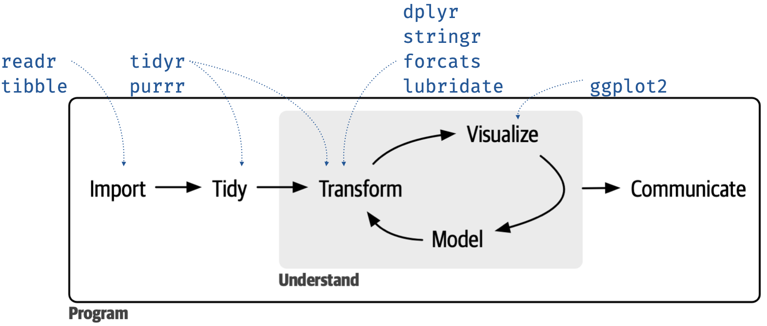
You've already learned **SO MUCH** in this class:
. . .
{fig-align="center"}
. . .
But if grad school teaches us anything, it's that the more we learn, the more we realize how much more there is to learn. 🥴😑🫠
---
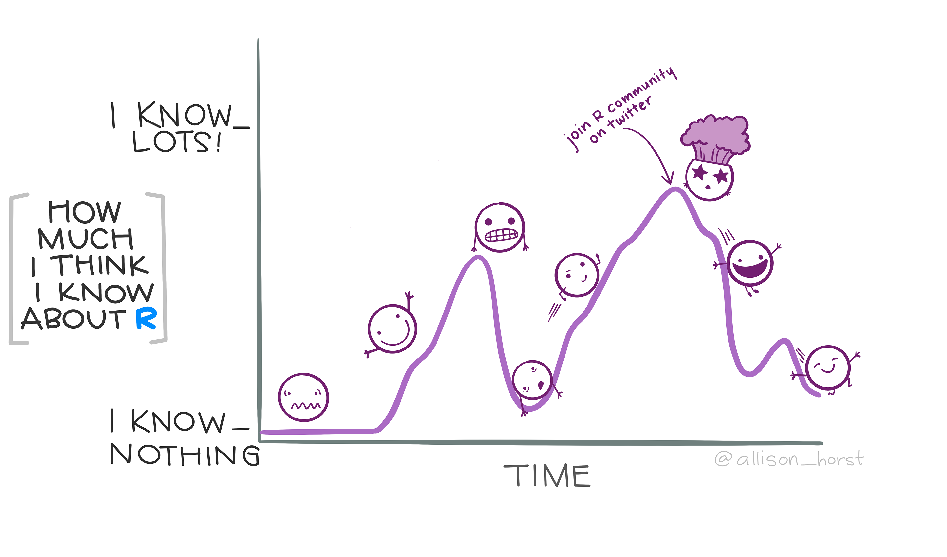
This can be freeing! And even fun?! Let your curiosity run wild!
{fig-align="center"}
---
Today, we'll look at some of the ways you can extend your learning beyond the scope of this introductory course.
::: {.incremental}
* Tidy modeling
* Even more visualizations
* Creating web applications
* Version control with Git/GitHub
* Creating slides, articles, books, and/or websites
:::
# Tidy Modeling{.section-title background-color="#99a486"}
## Modeling in R
{fig-align="center"}
## Modeling with `tidymodels`
```{r}
#| message: true
library(tidymodels)
```
::: aside
[Tidymodels is best suited for **predictive** modeling, which can be useful even if your main goal is *causal* inference (i.e. anomaly/outlier detection via machine learning techniques to impute missing values of an important variable)]{.fragment}
:::
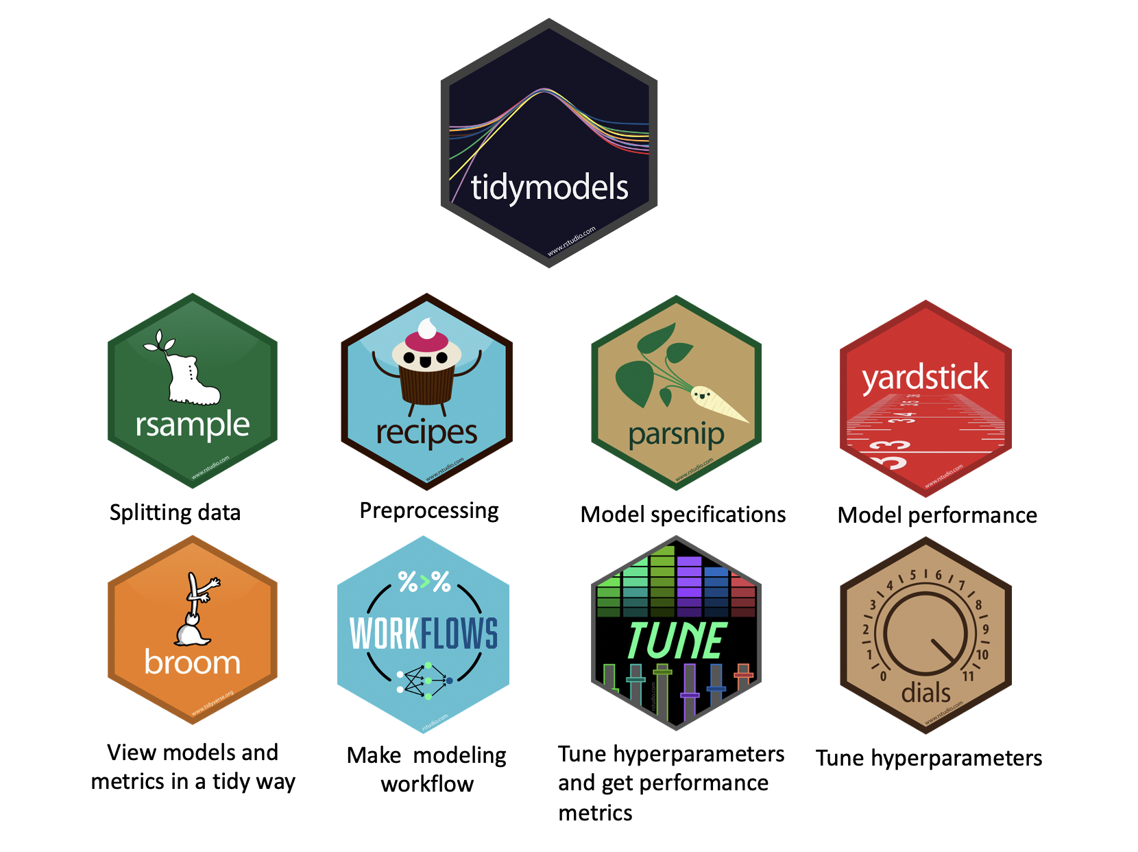
## `tidymodels` Packages
{fig-align="center"}
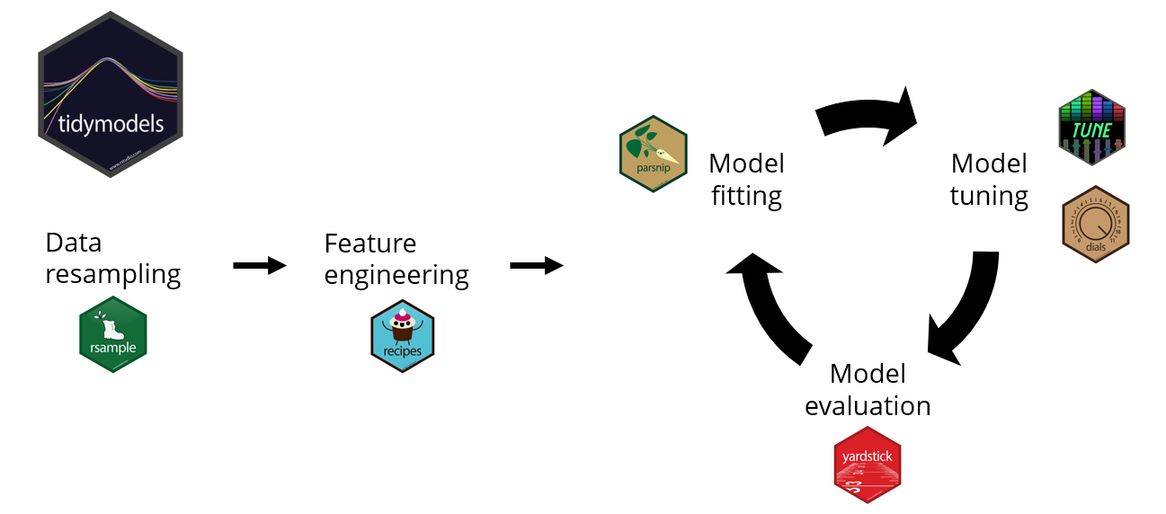
## `tidymodels` Approach
{fig-align="center"}
## Packages Using Tidymodels Framework [{{< fa scroll >}}]{style="color:#99a486"} {.scrollable}
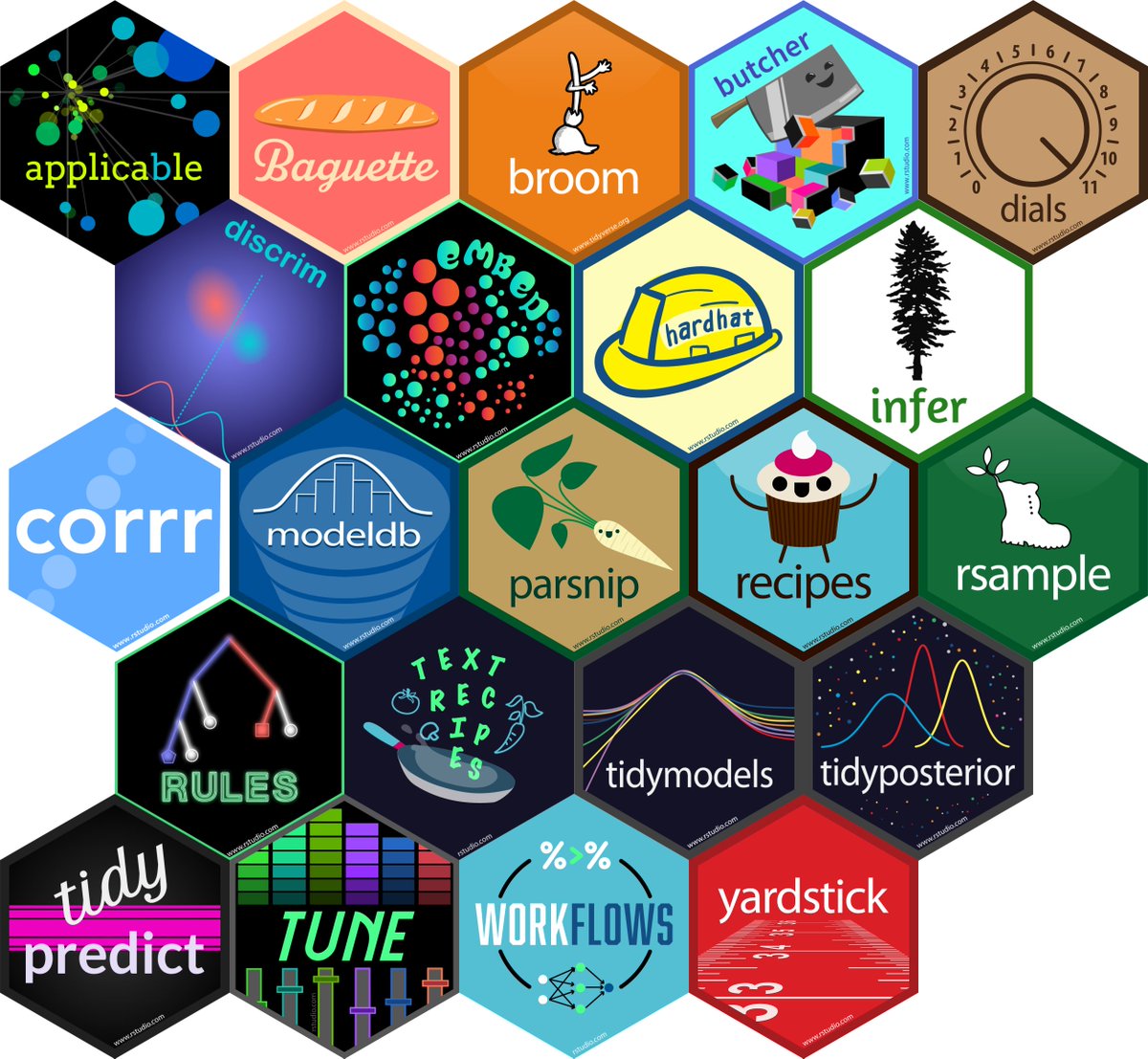{fig-align="center" width=60% height=60%}
::: aside
1. `applicable` compares new data points with the training data to see how much the new data points appear to be an extrapolation of the training data
2. `baguette` is for speeding up bagging pipelines
3. `butcher` is for dealing with pipelines that create model objects that take up too much memory
4. `discrim` has more model options for classification
5. `embed` has extra preprocessing options for categorical predictors
6. `hardhat` helps you to make new modeling packages
7. `corrr` has more options for looking at correlation matrices
8. `rules` has more model options for prediction rule ensembles
9. `text` recipes has extra preprocessing options for using text data
10. `tidypredict` is for running predictions inside SQL databases
11. `modeldb` is also for working within SQL databases and it allows for dplyr and tidyeval use within a database
12. `tidyposterior` compares models using resampling statistics
:::
## `tidymodels` Resources
::: {.incremental}
1. The [website for `tidymodels`](https://www.tidymodels.org/) has extensive documentation on all core `tidymodels` packages as well as related ones.^[They also provide a [great introductory tutorial](https://www.tidymodels.org/start/) to lay out the framework for why and how to use each core `tidymodels` package.]
2. There is an excellent book online by Max Kuhn and Julia Silge called [Tidy Modeling with R](https://www.tmwr.org/) that provides a great overview of how to approach modeling within a tidy framework and well as showing how to use the various packages within `tidymodels`.
3. Additionally, there are also several related, online book resources:
* [Feature Engineering & Selection: A Practical Approach for Predictive Models](https://bookdown.org/max/FES/) by Max Kuhn and Kjell Johnson
* [Statistical Inference via Data Science: A Modern Dive into R and the Tidyverse](https://moderndive.com/) by Chester Ismay and Albert Y. Kim
* [Supervised Machine Learning for Text Analysis in R](https://smltar.com/) by Emil Hvitfeldt and Julia Silge
* [Text Mining with R: A Tidy Approach](https://www.tidytextmining.com/) by Julia Silge & David Robinson
:::
# Even More Visualizations{.section-title background-color="#99a486"}
## Spatial Data with `ggmap`
There are numerous ways to work with spatial data in `R` but you can use `ggmap` to visualize spatial data in a tidyverse framework.
. . .
```{r}
source("stadia_api_key.R") # <1>
library(ggmap)
`%notin%` <- function(lhs, rhs) !(lhs %in% rhs) # <2>
violent_crimes <- crime |> # <3>
filter(offense %notin% c("auto theft", "theft", "burglary"),
between(lon, -95.39681, -95.34188),
between(lat, 29.73631, 29.78400)) |>
mutate(offense = fct_drop(offense),
offense = fct_relevel(offense,
c("robbery", "aggravated assault", "rape", "murder")))
```
1. You need to register for Stadia Maps or Google Maps and get a respective API key in order to download their maps. This `R` script simply saves my API key and registers it in the current session so it's not included in my code that's accessible on GitHub.
2. Creating a helper function that negates the %in% function.
3. `crime` is a built-in dataset in the `ggmap` package.
## Making a Map
Once we have data we want to visualize we can call `ggmap` to visualize the spatial area and layer on any geoms/stats as you would with `ggplot2.`
. . .
:::: {.columns}
::: {.column width="50%"}
```{r}
#| eval: false
bbox <- make_bbox(lon, lat, # <1>
data = violent_crimes) # <1>
map <- get_stadiamap(bbox = bbox, # <2>
maptype = "stamen_toner_lite", # <2>
zoom = 14) # <2>
ggmap(map) +
geom_point(data = violent_crimes, # <3>
color = "red") # <3>
```
1. Creating the bounding box for the longitude and latitude.
2. Retrieving the map with specifications.
3. The only difference with layers using `ggmap` is that (1) you need to specify the data arguments in the layers and (2) the spatial aesthetics `x` and `y` are set to `lon` and `lat`, respectively. (If they’re named something different in your dataset, just put `mapping = aes(x = longitude, y = latitude)`, for example.)
:::
::: {.column width="50%"}
```{r}
#| echo: false
#| fig-align: center
#| fig-width: 7
#| fig-height: 7
#| code-line-numbers: false
bbox <- make_bbox(lon, lat,
data = violent_crimes)
map <- get_stadiamap( bbox = bbox,
maptype = "stamen_toner_lite",
zoom = 14 )
ggmap(map) +
geom_point(data = violent_crimes,
color = "red")
```
:::
::::
## Using Different Geoms
With `ggmap` you’re working with `ggplot2`, so you can add in other kinds of layers, use `patchwork`, etc. All the `ggplot2` geom’s are available.
. . .
```{r}
#| output-location: slide
#| fig-align: center
#| fig-height: 10
#| fig-width: 15
library(patchwork)
library(ggdensity)
library(geomtextpath)
robberies <- violent_crimes |> filter(offense == "robbery")
points_map <- ggmap(map) + geom_point(data = robberies, color = "red")
hdr_map <- ggmap(map) +
geom_hdr(aes(lon, lat, fill = after_stat(probs)),
data = robberies,
alpha = .5) +
geom_labeldensity2d(aes(lon, lat, level = after_stat(probs)),
data = robberies,
stat = "hdr_lines",
size = 3, boxcolour = NA) +
scale_fill_brewer(palette = "YlOrRd") +
theme(legend.position = "none")
(points_map + hdr_map) &
theme(axis.title = element_blank(), axis.text = element_blank(), axis.ticks = element_blank())
```
## Marginal Histogram
```{r}
#| output-location: fragment
#| fig-align: center
library(ggExtra)
data(mpg, package = "ggplot2")
mpg_select <- mpg |>
filter(hwy >= 35 & cty > 27)
g <- ggplot(mpg, aes(cty, hwy)) +
geom_count() +
geom_smooth(method = "lm", se = F) +
theme_bw()
ggMarginal(g, type = "histogram", fill = "transparent") # <1>
```
1. Code that adds marginal plot.
## Marginal Boxplot
```{r}
#| fig-align: center
library(ggExtra)
data(mpg, package = "ggplot2")
mpg_select <- mpg |>
filter(hwy >= 35 & cty > 27)
g <- ggplot(mpg, aes(cty, hwy)) +
geom_count() +
geom_smooth(method = "lm", se = F) +
theme_bw()
ggMarginal(g, type = "boxplot", fill = "transparent") # <1>
```
1. Code that adds marginal plot.
## Marginal Density Curve
```{r}
#| fig-align: center
library(ggExtra)
data(mpg, package = "ggplot2")
mpg_select <- mpg |>
filter(hwy >= 35 & cty > 27)
g <- ggplot(mpg, aes(cty, hwy)) +
geom_count() +
geom_smooth(method = "lm", se = F) +
theme_bw()
ggMarginal(g, type = "density", fill = "transparent") # <1>
```
1. Code that adds marginal plot.
## Create Animations
```{r}
#| eval: false
library(gapminder)
library(gganimate)
library(gifski) # <1>
ggplot(gapminder, aes(gdpPercap, lifeExp, size = pop, colour = country)) +
geom_point(alpha = 0.7, show.legend = FALSE) +
scale_colour_manual(values = country_colors) +
scale_size(range = c(2, 12)) +
scale_x_log10() +
facet_wrap(~continent) +
labs(title = 'Year: {frame_time}', x = 'GDP per capita', y = 'life expectancy') + # <2>
transition_time(year) + # <2>
ease_aes('linear') # <2>
```
1. Need this package to create a gif of the `gganimate` output.
2. `gganimate`-specific code.
## Create Animations
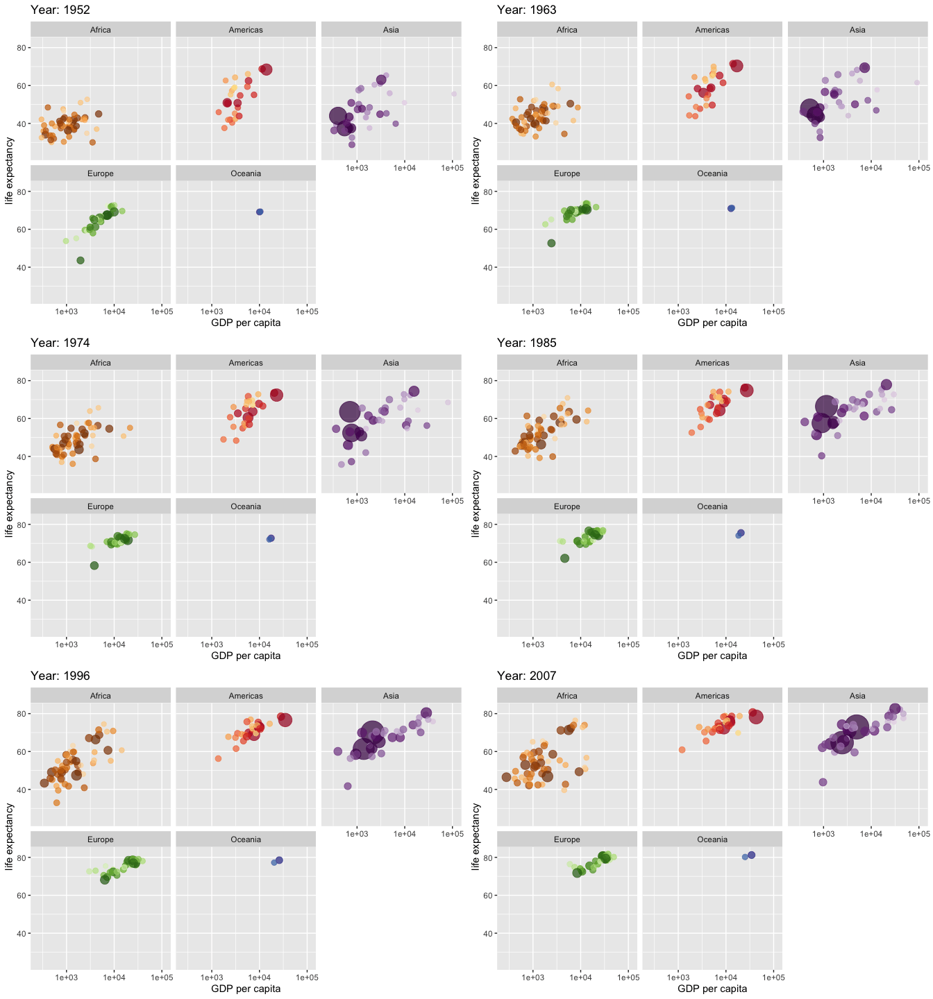{fig-align="center"}
## Data Visualization Resources
::: {.incremental}
1. Hadley Wickham's *`ggplot2`: Elegant Graphics for Data Analysis (Second Edition)* is available through the [UW Library](https://orbiscascade-washington.primo.exlibrisgroup.com/permalink/01ALLIANCE_UW/1juclfo/alma99161977549501452) and the forthcoming [Third Edition](https://ggplot2-book.org/) is being written as we speak and will be available online soon!
2. [Spatial Data Science with Applications in R](https://r-spatial.org/book/) by Edzer Pebesma and Roger Bivand
3. The [`sf`](https://r-spatial.github.io/sf/) package also works within the tidyverse framework and pairs very nicely with data from the census which can be easily accessed using [`tidycensus`](https://walker-data.com/tidycensus/)
4. More ideas for visualizations can be found on [this master list](https://r-statistics.co/Top50-Ggplot2-Visualizations-MasterList-R-Code.html) and by looking at [ggplot2 extension packages](https://exts.ggplot2.tidyverse.org/gallery/).
5. Think about taking **CSSS 569** with Chris Adolph (offered in Winter quarter) if you want to learn more about how to create visualizations in `R` and gain more understanding about best practices for conveying your data and findings effectively.
:::
# Creating web applications{.section-title background-color="#99a486"}
## Shiny
Shiny is an open source R package that provides an elegant and powerful web framework for building web applications using R. Shiny helps you turn your analyses into interactive web applications without requiring HTML, CSS, or JavaScript knowledge.
. . .
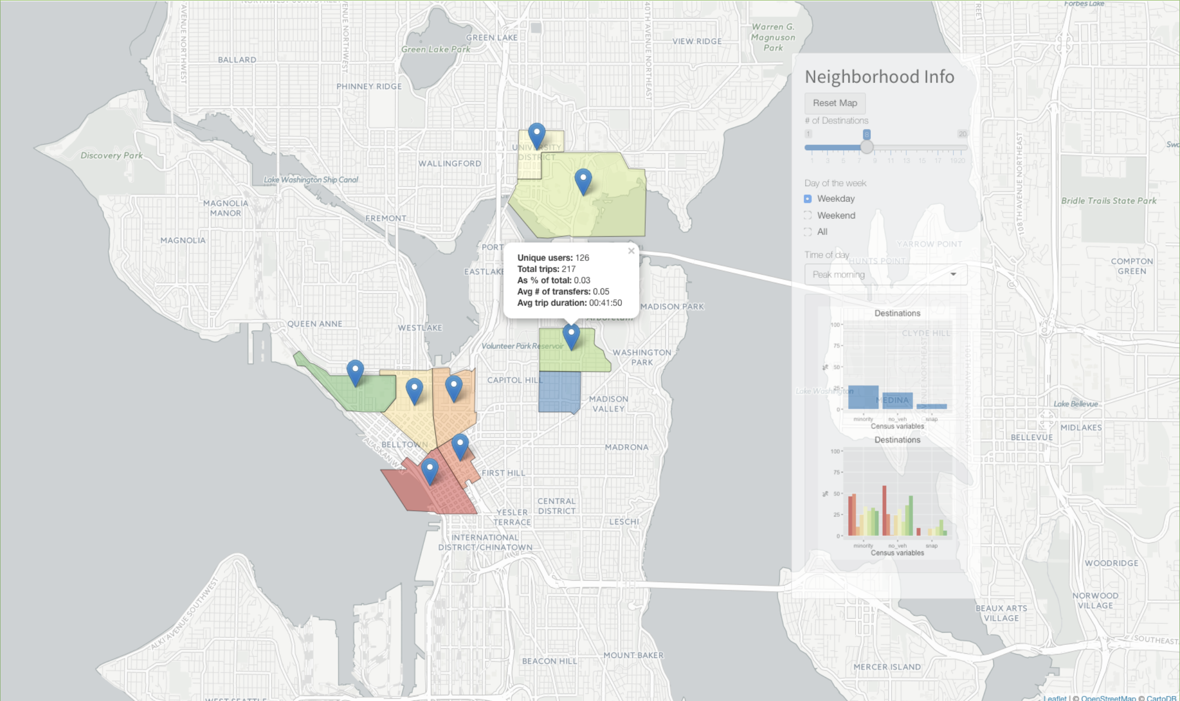{fig-align="center" height="80%" width="80%"}
## Shiny Examples{background-iframe="https://shiny.posit.co/r/gallery/#feature-demos" background-interactive="true"}
# Version control with Git/GitHub{.section-title background-color="#99a486"}
## What is Version Control?
Version control allows you to work work individually and/or collaboratively in a highly structured, documented way.
. . .
It's basically like a robust save program for your project. You track and log changes you make over time and the version control system allows you to review or even restore earlier versions of your project.
. . .
:::: {.columns}
::: {.column width="50%"}
Originally meant for software developers, git has been adopted by computational social scientists to source code but also to keep track of the whole collection of files that make up a research project.
:::
::: {.column width="50%"}
{fig-align="center"}
:::
::::
. . .
## Why Use Version Control?
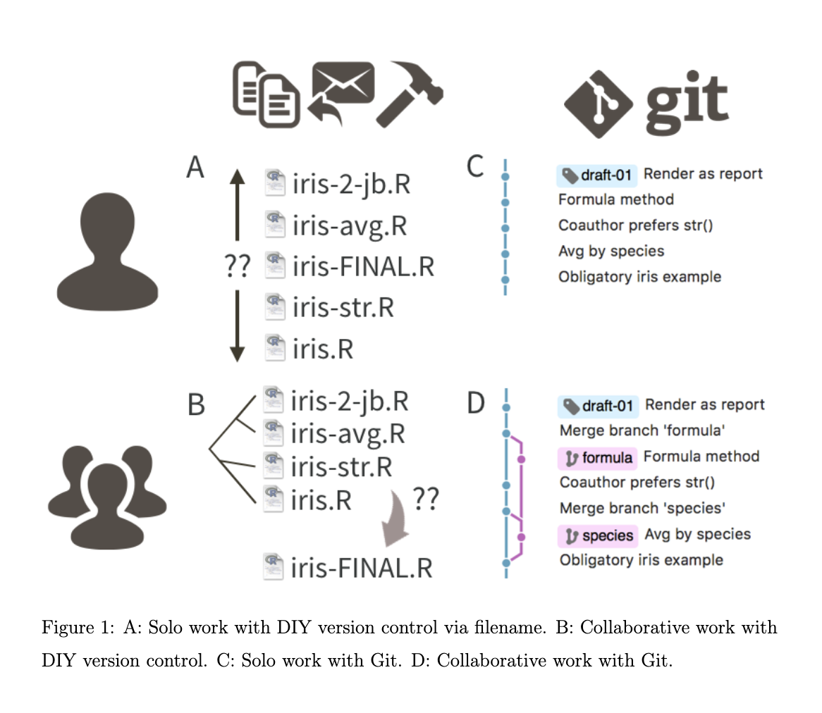{fig-align="center"}
## What is Github?
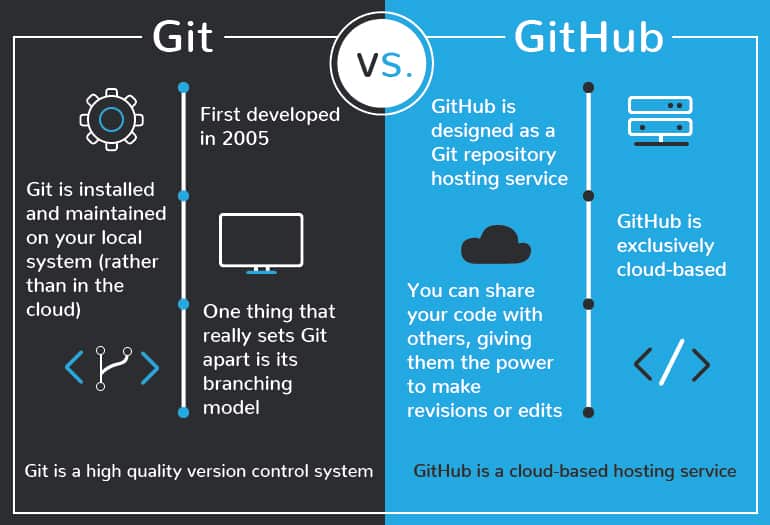{fig-align="center"}
## Why Use Github?
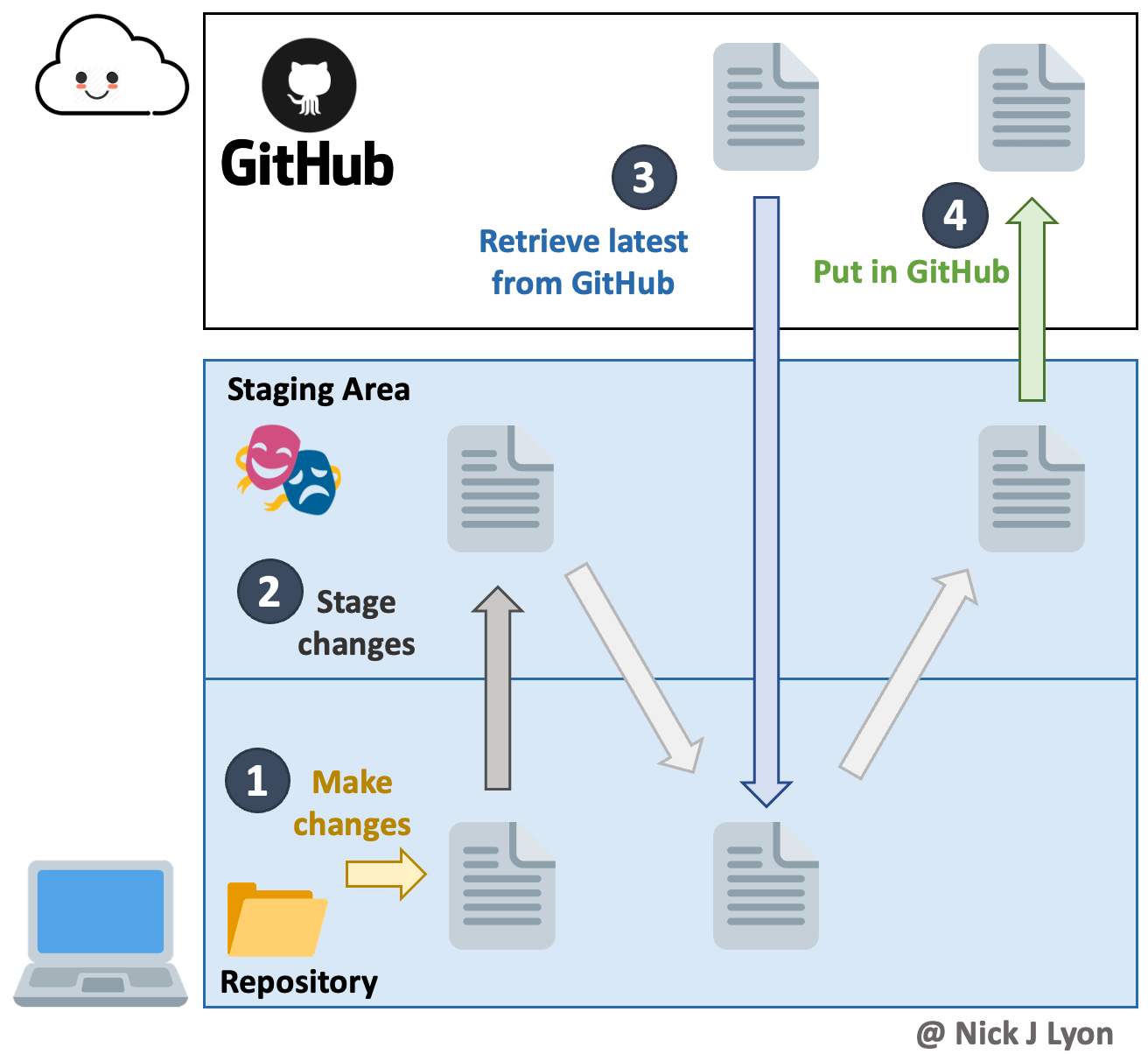{fig-align="center"}
## Collaboration Made "Easier"
:::: {.columns}
::: {.column width="40%"}
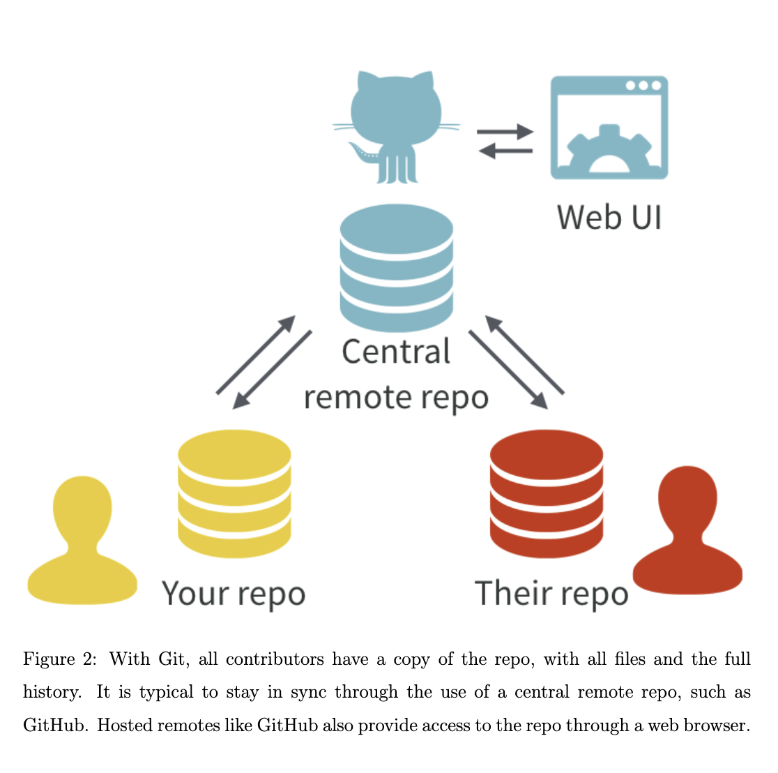{fig-align="center"}
:::
::: {.column width="60%"}
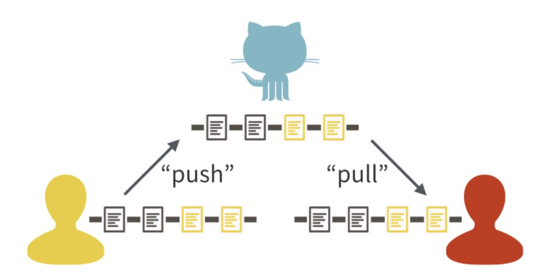{fig-align="center"}
:::
::::
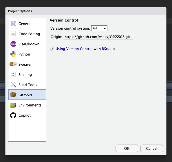
## Git Integration in R Studio
{fig-align="center"}
## Git/GitHub Resources
::: {.incremental}
1. Hands down the best introduction to git and using git/GitHub with RStudio Projects is Jennifer Bryan's online book [Happy Git and GitHub for the useR](https://happygitwithr.com/)
2. Software carpentry has a nice [beginner's "class"](https://swcarpentry.github.io/git-novice/) that'll help you learn the git basics.
3. Here's a user-contributed cheat-sheet for [Using git and GitHub with RStudio](https://rstudio.github.io/cheatsheets/git-github.pdf).
:::
# Creating slides, articles, books, and/or websites{.section-title background-color="#99a486"}
## Quarto{background-iframe="https://quarto.org/docs/guide/" background-interactive="true"}
# That's a Wrap! {.section-title background-color="#99a486"}
## Plug for CSSCR
Also, this lab is part of CSSCR ([The Center for Social Science Computation and Research](https://depts.washington.edu/csscr/)) where I'm also on staff as a consultant. CSSCR is a resource center for the social science departments^[Constituent member departments include The College of Education, The Department of Anthropology, The Department of Communication, The Department of Economics, The Department of Geography, The Department of Political Science, The Department of Psychology, The Department of Sociology, The Jackson School of International Studies, and The School of Social Work] at the University of Washington.
As you continue to learn `R` feel free to drop by^[We offer drop-in consulting in Savery 119, 8am-6pm Monday-Friday.] with any/all of your `R` coding questions.
---
Thanks for spending so much time this quarter learning with me 😎
{fig-align="center"}
Don't forget to fill out the course evaluation that you received via email!