---
execute:
echo: true
message: false
warning: false
fig-format: "svg"
format:
revealjs:
highlight-style: a11y-dark
reference-location: margin
theme: lecture_styles.scss
controls: true
controls-tutorial: true
slide-number: true
code-link: true
chalkboard: true
incremental: false
smaller: true
preview-links: true
code-line-numbers: true
history: false
progress: true
link-external-icon: true
code-annotations: hover
pointer:
color: "#b18eb1"
revealjs-plugins:
- pointer
---
```{r}
#| echo: false
#| cache: false
require(downlit)
require(xml2)
require(tidyverse)
library(gapminder)
#options(width = 90)
```
## {#title-slide data-menu-title="Manipulating and Summarizing Data" background="#1e4655" background-image="../../images/csss-logo.png" background-position="center top 5%" background-size="50%"}
[Manipulating and Summarizing Data]{.custom-title}
[CS&SS 508 • Lecture 4]{.custom-subtitle}
[{{< var lectures.four >}}]{.custom-subtitle2}
[Victoria Sass]{.custom-subtitle3}
# Roadmap{.section-title background-color="#99a486"}
---
:::: {.columns}
::: {.column width="50%"}
### Last time, we learned:
* Best Practices
* Code Style
* Workflow
* Reproducible Research
* Indexing vectors & dataframes in Base `R`
:::
::: {.column width="50%"}
::: {.fragment}
### Today, we will cover:
* Types of Data
* Logical Operators
* Subsetting data
* Modifying data
* Summarizing data
* Merging data
:::
:::
::::
. . .
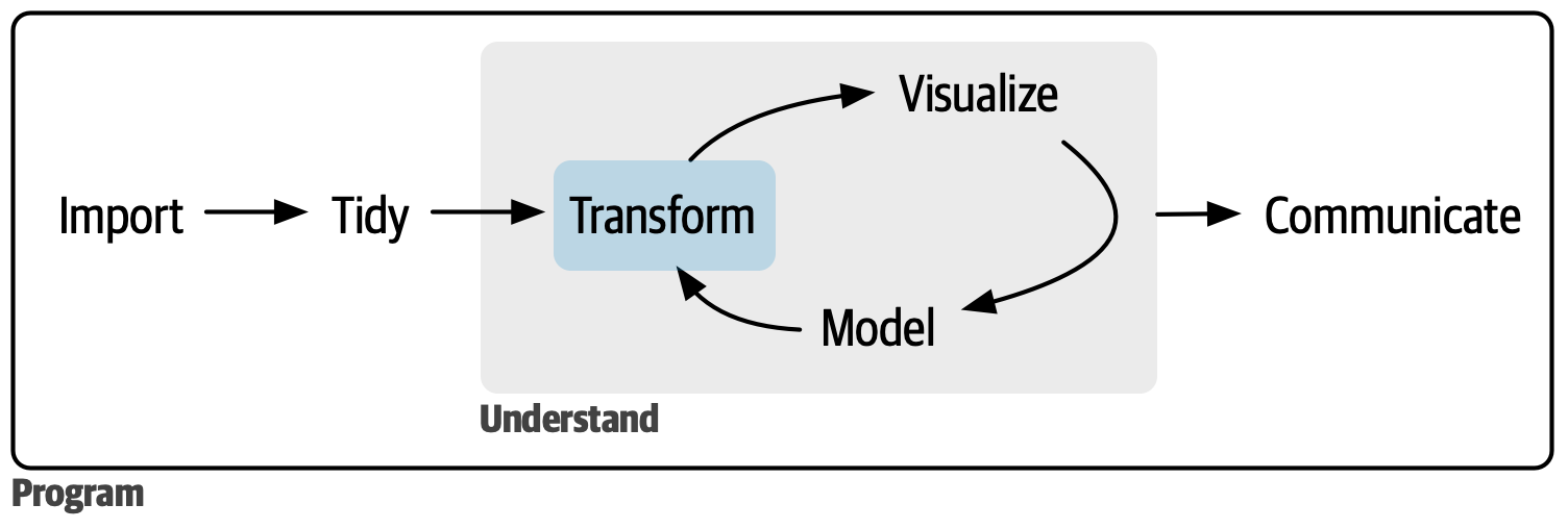{fig-align="center"}
## Death to Spreadsheets
Tools like *Excel* or *Google Sheets* let you manipulate spreadsheets using functions.
::: {.incremental}
* Spreadsheets are *not reproducible*: It's hard to know how someone changed the raw data!
* It's hard to catch mistakes when you use spreadsheets^[Don't be the next sad Research Assistant who makes headlines with an Excel error! ([Reinhart & Rogoff, 2010](http://www.bloomberg.com/news/articles/2013-04-18/faq-reinhart-rogoff-and-the-excel-error-that-changed-history))].
:::
. . .
Today, we'll use `R` to manipulate data more *transparently* and *reproducibly*.
## How is data stored in `R`?
Under the hood, R stores different types of data in different ways.
. . .
* e.g., R knows that `4.0` is a number, and that `"Vic"` is not a number.
. . .
So what exactly are the common data types, and how do we know what R is doing?
. . .
:::: {.columns}
::: {.column width="50%"}
* Logicals (`logical`)
* Factors (`factor`)
* Date/Date-time (`Date`, `POSIXct`, `POSIXt`)
* Numbers (`integer`, `double`)
* Missing Values (`NA`, `NaN`, `Inf`)
* Character Strings (`character`)
:::
::: {.column width="50%"}
::: {.fragment}
* `c(FALSE, TRUE, TRUE)`
* `factor(c("red", "blue"))`
* `as_Date(c("2018-10-04"))`
* `c(1, 10*3, 4, -3.14)`
* `c(NA, NA, NA, NaN, NaN, NA)`
* `c("red", "blue", "blue")`
:::
:::
::::
# Logical Operators{.section-title background-color="#99a486"}
## Booleans
The simplest data type is a Boolean, or binary, variable: `TRUE` or `FALSE`^[or `NA`].
. . .
More often than not our data don't actually have a variable with this data type, but they are definitely created and evaluated in the data manipulation and summarizing process.
. . .
Logical operators refer to base functions which allow us to **test if a condition** is present between two objects.
. . .
For example, we may test
+ Is A equal to B?
+ Is A greater than B?
+ Is A within B?
. . .
Naturally, these types of expressions produce a binary outcome of `T` or `F` which enables us to transform our data in a variety of ways!
## Logical Operators in `R`
#### Comparing objects
:::: {.columns}
::: {.column width="19%"}
::: {.fragment}
* `==`:
* `!=`:
* `>`, `>=`, `<`, `<=`:
* `%in%`:
:::
:::
::: {.column width="81%"}
::: {.fragment}
* is equal to^[Note: there are TWO equal signs here!]
* not equal to
* less than, less than or equal to, etc.
* used when checking if equal to one of several values
:::
:::
::::
:::{.fragment}
#### Combining comparisons
:::
:::: {.columns}
::: {.column width="19%"}
::: {.fragment}
* `&`:
* `|`:
* `!`:
* `xor()`:
:::
:::
::: {.column width="81%"}
::: {.fragment .bullet-spacing}
* **both** conditions need to hold (AND)\
* **at least one** condition needs to hold (OR)\
* **inverts** a logical condition (`TRUE` becomes `FALSE`, vice versa)\
* **exclusive OR** (i.e. x or y but NOT both)
:::
:::
::::
::: {.aside}
[You may also see `&&` and `||` but they are what's known as short-circuiting operators and are not to be used in `dplyr` functions (used for programming not data manipulation); they'll only ever return a single `TRUE` or `FALSE`.]{.fragment}
:::
## Unexpected Behavior
Be careful using `==` with numbers:
. . .
```{r}
(x <- c(1 / 49 * 49, sqrt(2) ^ 2)) # <1>
```
1. Wrapping an entire object assignment in parentheses simultaneously defines the object and shows you what it represents.
```{r}
x == c(1, 2) # <2>
print(x, digits = 16) # <3>
```
2. Computers store numbers with a fixed number of decimal places so there’s no way to *precisely* represent decimals.
3. `dplyr::near()` is a useful alternative which ignores small differences.
. . .
Similarly mysterious, missing values (`NA`) represent the unknown. Almost anything conditional involving `NA`s will also be unknown:
```{r}
NA > 5
10 == NA
NA == NA # <4>
```
4. The logic here: if you have one unknown and a second unknown, you don't actually know if they equal one another!
. . .
This is the reason we use `is.na()` to check for missingness.
```{r}
is.na(c(NA, 5))
```
## Examples of Logical Operators
Let's create two objects, `A` and `B`
```{r}
A <- c(5, 10, 15)
B <- c(5, 15, 25)
```
. . .
Comparisons:
```{r}
A == B
A > B
A %in% B # <1>
```
1. Will return a vector the length of `A` that is `TRUE` whenever a value in `A` is anywhere in `B`.
**Note**: You CAN use `%in%` to search for `NA`s.
. . .
Combinations:
```{r}
A > 5 & A <= B
B < 10 | B > 20 # <2>
!(A == 10)
```
2. Be sure not to cut corners (i.e. writing
`B < 10 | > 20`). The code won't technically error but it won't evaluate the way you expect it to. Read more about the confusing logic behind this [here](https://r4ds.hadley.nz/logicals#sec-order-operations-boolean). In essence the truncated second part of this conditional statement (> 20) will evaluate to `TRUE` since any numeric that isn't `0` for a logical operator is coerced to `TRUE`. Therefore this statement will actually always evaluate to `TRUE` and will return all elements of `B` instead of the ones that meet your specified condition.
## Logical Summaries
:::: {.columns}
::: {.column width="19%"}
::: {.fragment}
* `any()`:
* `all()`:
:::
:::
::: {.column width="81%"}
::: {.fragment}
* the equivalent of `|`; it’ll return `TRUE` if there are any `TRUE`’s in x
* the equivalent of `&`; it’ll return `TRUE` only if all values of x are `TRUE`’s
:::
:::
::::
. . .
\
```{r}
C <- c(5, 10, NA, 10, 20, NA)
any(C <= 10)
```
. . .
```{r}
all(C <= 20) # <1>
```
1. Like other summary functions, they'll return `NA` if there are any missing values present and it's `FALSE`.
. . .
```{r}
all(C <= 20, na.rm = TRUE) # <2>
```
2. Use `na.rm = TRUE` to remove `NA`s prior to evaluation.
. . .
```{r}
mean(C, na.rm = TRUE) # <3>
```
3. When you evaluate a logical vector numerically, `TRUE` = 1 and `FALSE` = 0. This makes `sum()` and `mean()` useful when summarizing logical functions (sum gives number of `TRUE`s and mean gives the proportion).
## Conditional transformations
**`if_else()`**
If you want to use one value when a condition is `TRUE` and another value when it’s `FALSE`.
. . .
```{r}
#| eval: false
if_else(condition = "A logical vector", # <1>
true = "Output when condition is true", # <1>
false = "Output when condition is false") # <1>
```
1. All of these arguments are required.
. . .
```{r}
x <- c(-3:3, NA)
if_else(x > 0, "+ve", "-ve", "???") # <2>
```
2. There’s an optional fourth argument, `missing`, which will be used if the input is `NA`.
. . .
**`case_when()`**
A very useful extension of `if_else()` for multiple conditions^[Note that if multiple conditions match in `case_when()`, only the first will be used.
].
. . .
```{r}
case_when(
x == 0 ~ "0",
x < 0 ~ "-ve",
x > 0 ~ "+ve",
is.na(x) ~ "???" # <3>
) # <4>
```
3. Use `.default` if you want to create a “default”/catch all value.
4. Both functions require compatible types: i.e. numerical and logical, strings and factors, dates and datetimes, `NA` and everything.
# {data-menu-title="`dplyr`" background-image="images/dplyr.png" background-size="contain" background-position="center" .section-title background-color="#1e4655"}
## `dplyr`
Today, we'll use tools from the `dplyr` package to manipulate data!
* Like `ggplot2`, `dplyr` is part of the *Tidyverse*, and included in the `tidyverse` package.
```{r}
library(tidyverse)
```
. . .
To demonstrate data transformations we're going to use the `nycflights13` dataset, which you'll need to download and load into `R`
```{r}
library(nycflights13) # <1>
```
1. Run `install.packages("nycflights13")` in console first.
. . .
`nycflights13` includes five data frames^[Note these are separate data frames, each needing to be loaded separately. When loading a package containing datasets, you can define those data (i.e. explicitly add them to your working environment) by calling `data()` on their name.]:, some of which contain missing data (`NA`):
```{r}
#| eval: false
data(flights) # <2>
data(airlines) # <3>
data(airports) # <4>
data(planes) # <5>
data(weather) # <6>
```
2. flights leaving JFK, LGA, or EWR in 2013
3. airline abbreviations
4. airport metadata
5. airplane metadata
6. hourly weather data for JFK, LGA, and EWR
## `dplyr` Basics
All `dplyr` functions have the following in common:
::: {.incremental}
1. The first argument is always a data frame.
2. The subsequent arguments typically describe which columns to operate on, using the variable names (without quotes).
3. The output is always a new data frame.
:::
. . .
Each function operates either on rows, columns, groups, or entire tables.
. . .
To save the transformations you've made to a data frame you'll need to save the output to a new object.
# Subsetting data{.section-title background-color="#99a486"}
## Subset Rows: `filter()`
We often get *big* datasets, and we only want some of the entries. We can subset rows using `filter()`.
. . .
```{r}
delay_2hr <- flights |>
filter(dep_delay > 120) # <1>
delay_2hr # <2>
```
1. Here's where all your new knowledge about logical operators comes in handy! Make sure to use `==` not `=` to test the logical condition.
2. Now, `delay_2hr` is an object in our environment which contains rows corresponding to flights that experienced at least a 2 hour delay.
## Subset Columns: `select()`
What if we want to keep every observation, but only use certain variables? Use `select()`!
. . .
We can select columns by name:
```{r}
flights |>
select(year, month, day) # <1>
```
1. You can use a `-` before a variable name or a vector of variables to drop them from the data (i.e.
`select(-c(year, month, day))`).
## Subset Columns: `select()`
What if we want to keep every observation, but only use certain variables? Use `select()`!
We can select columns between variables (inclusive):
```{r}
flights |>
select(year:day) # <1>
```
1. Add a `!` before `year` and you'll drop this group of variables from the data.
## Subset Columns: `select()`
What if we want to keep every observation, but only use certain variables? Use `select()`!
We can select columns based on a condition:
```{r}
flights |>
select(where(is.character)) # <1>
```
1. There are a number of helper functions you can use with `select()` including `starts_with()`, `ends_with()`, `contains()` and `num_range()`. Read more about these and more [here](https://tidyselect.r-lib.org/reference/index.html).
## Finding Unique Rows: `distinct()`
You may want to find the unique combinations of variables in a dataset. Use `distinct()`
. . .
```{r}
flights |>
distinct(origin, dest) # <1>
```
1. Find all unique origin and destination pairs.
## `distinct()` drops variables!
By default, `distinct()` drops unused variables. If you don't want to drop them, add the argument `.keep_all = TRUE`:
. . .
```{r}
flights |>
distinct(origin, dest, .keep_all = TRUE) # <1>
```
1. It’s not a coincidence that all of these distinct flights are on January 1: `distinct()` will find the first occurrence of a unique row in the dataset and discard the rest. Use `count()` if you're looking for the number of occurrences.
## Count Unique Rows: `count()`
. . .
```{r}
flights |>
count(origin, dest, sort = TRUE) # <1>
```
1. `sort = TRUE` arranges them in descending order of number of occurrences.
# Modifying data{.section-title background-color="#99a486"}
## Sorting Data by Rows: `arrange()`
Sometimes it's useful to sort rows in your data, in ascending (low to high) or descending (high to low) order. We do that with `arrange()`.
. . .
```{r}
flights |>
arrange(year, month, day, dep_time) # <1>
```
1. If you provide more than one column name, each additional column will be used to break ties in the values of preceding columns.
## Sorting Data by Rows: `arrange()`
To sort in descending order, using `desc()` within `arrange()`
. . .
```{r}
flights |>
arrange(desc(dep_delay))
```
## Rename Variables: `rename()`
You may receive data with unintuitive variable names. Change them using `rename()`.
. . .
```{r}
flights |>
rename(tail_num = tailnum) # <1>
```
1. `rename(new_name = old_name)` is the format. Reminder to use `janitor::clean_names()` if you want to automate this process for a lot of variables.
. . .
::: {.callout-caution icon=false}
## {{< fa exclamation-triangle >}} Variable Syntax
I recommend **against** using spaces in a name! It makes things *really hard* sometimes!!
:::
## Create New Columns: `mutate()`
You can add new columns to a data frame using `mutate()`.
. . .
```{r}
flights |>
mutate(
gain = dep_delay - arr_delay,
speed = distance / air_time * 60,
.before = 1 # <1>
)
```
1. By default, `mutate()` adds new columns on the right hand side of your dataset, which makes it difficult to see if anything happened. You can use the `.before` argument to specify which numeric index (or variable name) to move the newly created variable to. `.after` is an alternative argument for this.
## Specifying Variables to Keep: `mutate()`
You can specify which columns to keep with the `.keep` argument:
```{r}
flights |>
mutate(
gain = dep_delay - arr_delay,
hours = air_time / 60,
gain_per_hour = gain / hours,
.keep = "used" # <1>
)
```
1. `"used"` retains only the variables used to create the new variables, which is useful for checking your work. Other options include: `"all"` (default, returns all columns), `"unused"` (columns not used to create new columns) and `"none"` (only grouping variables and columns created by mutate are retained).
## Move Variables Around: `relocate()`
You might want to collect related variables together or move important variables to the front. Use `relocate()`!
```{r}
flights |>
relocate(time_hour, air_time) # <1>
```
1. By default `relocate()` moves variables to the front but you can also specify where to put them using the `.before` and `.after` arguments, just like in `mutate()`.
# Summarizing data{.section-title background-color="#99a486"}
## Grouping Data: `group_by()`
If you want to analyze your data by specific groupings, use `group_by()`:
```{r}
flights |>
group_by(month) # <1>
```
1. `group_by()` doesn’t change the data but you’ll notice that the output indicates that it is “grouped by” month `(Groups: month [12])`. This means subsequent operations will now work “by month”.
## Summarizing Data: `summarize()`
**`summarize()`** calculates summaries of variables in your data:
::: {.incremental}
* Count the number of rows
* Calculate the mean
* Calculate the sum
* Find the minimum or maximum value
:::
. . .
You can use any function inside `summarize()` that aggregates *multiple values* into a *single value* (like `sd()`, `mean()`, or `max()`).
## `summarize()` Example
Let's see what this looks like in our flights dataset:
. . .
```{r}
flights |>
summarize(
avg_delay = mean(dep_delay) # <1>
)
```
1. The `NA` produced here is a result of calling `mean` on `dep_delay`. Any summarizing function will return `NA` if **any** of the values are `NA`. We can set `na.rm = TRUE` to change this behavior.
## `summarize()` Example
Let's see what this looks like in our flights dataset:
```{r}
flights |>
summarize(
avg_delay = mean(dep_delay, na.rm = TRUE)
)
```
## Summarizing Data by Groups
What if we want to summarize data by our groups? Use `group_by()` **and** `summarize()`
. . .
```{r}
flights |>
group_by(month) |>
summarize(
delay = mean(dep_delay, na.rm = TRUE)
)
```
. . .
Because we did `group_by()` *with* `month`, *then* used `summarize()`, we get **one row per value of `month`**!
## Summarizing Data by Groups
You can create any number of summaries in a single call to summarize().
```{r}
flights |>
group_by(month) |>
summarize(
delay = mean(dep_delay, na.rm = TRUE),
n = n() # <1>
)
```
1. `n()` returns the number of rows in each group.
## Grouping by Multiple Variables {{< fa scroll >}} {.scrollable}
```{r}
daily <- flights |>
group_by(year, month, day)
daily
```
. . .
::: {.callout-tip icon=false}
## {{< fa info-circle >}} Summary & Grouping Behavior
When you summarize a tibble grouped by more than one variable, each summary peels off the last group. You can change the default behavior by setting the `.groups` argument to a different value, e.g., `"drop"` to drop all grouping or `"keep"` to preserve the same groups. The default is `"drop_last"` if all groups have 1 row and `keep` otherwise (it's recommended to use `reframe()` if this is the case, which is a more general version of `summarize()` that allows for an arbitrary number of rows per group and drops all grouping variables after execution).
:::
## Remove Grouping: `ungroup()`
```{r}
daily |>
ungroup()
```
## Newer Alternative for Grouping: `.by`
```{r}
flights |>
summarize(
delay = mean(dep_delay, na.rm = TRUE),
n = n(),
.by = month # <1>
)
```
1. `.by` works with all verbs and has the advantage that you don’t need to use the `.groups` argument to suppress the grouping message or `ungroup()` when you’re done.
## Select Specific Rows Per Group: `slice_*`
There are five handy functions that allow you extract specific rows within each group:
::: {.incremental}
* `df |> slice_head(n = 1)` takes the first row from each group.
* `df |> slice_tail(n = 1)` takes the last row in each group.
* `df |> slice_min(x, n = 1)` takes the row with the smallest value of column x.
* `df |> slice_max(x, n = 1)` takes the row with the largest value of column x.
* `df |> slice_sample(n = 1)` takes one random row.
:::
. . .
Let's find the flights that are most delayed upon arrival at each destination.
## Select Specific Rows Per Group: `slice_*`
```{r}
flights |>
group_by(dest) |>
slice_max(arr_delay, n = 1) |> # <1>
relocate(dest, arr_delay)
```
1. You can vary `n` to select more than one row, or instead of `n`, you can use `prop` to select a proportion (between 0 and 1) of the rows in each group.
::: {.aside}
[There are 105 groups but 108 rows! Why? `slice_min()` and `slice_max()` keep tied values so `n = 1` means "give us all rows with the highest value." If you want exactly one row per group you can set `with_ties = FALSE`.]{.fragment}
:::
# Lab{.section-title background-color="#99a486"}
## Manipulating Data
1. Create a new object that contains the following from `gapminder`^[Using the `gapminder` package]
i. observations from China, India, and United States after 1980, *and*
ii. variables corresponding to country, year, population, and life expectancy.
1. How many rows and columns does the object contain?
1. Sort the rows by `year` (ascending order) and `population` (descending order) and save that over (i.e. overwrite) the object created for answer 1. Print the first 6 rows.
1. Create a new variable that contains population in billions.
1. By year, calculate the total population (in billions) across these three countries
1. In `ggplot`, create a line plot showing life expectancy over time by country. Make the plot visually appealing!
## Answers
Question 1:
```{r}
subset_gapminder <- gapminder |>
filter(country %in% c("China","India","United States"), year > 1980 ) |> # <1>
select(country, year, pop, lifeExp)
subset_gapminder
```
1. You can specify multiple conditional conditions in `filter()` by separating them with commas
## Answers
Question 2:
```{r}
# Option 1
c(nrow(subset_gapminder), ncol(subset_gapminder))
# Option 2
glimpse(subset_gapminder)
# Option 3
dim(subset_gapminder)
```
## Answers
Question 3:
```{r}
subset_gapminder <- subset_gapminder |>
arrange(year, desc(pop)) # <1>
```
1. The default for `arrange()` is to sort in ascending order
. . .
:::: {.columns}
::: {.column width="50%"}
```{r}
subset_gapminder |> head(6)
```
:::
::: {.column width="50%"}
```{r}
print(subset_gapminder[1:6, ])
```
:::
::::
## Answers
Question 4:
```{r}
subset_gapminder <- subset_gapminder |>
mutate(pop_billions = pop/1000000000)
subset_gapminder
```
## Answers
Question 5:
::: {.panel-tabset}
### Classic syntax
```{r}
subset_gapminder |>
group_by(year) |>
summarize(TotalPop_Billions = sum(pop_billions))
```
### New syntax (dplyr 1.1.0)
```{r}
subset_gapminder |>
summarize(TotalPop_Billions = sum(pop_billions),
.by = year) # <1>
```
1. This new syntax allows for per-operation grouping which means it is only active within a single verb at a time (as opposed to being applied to the entire tibble until `ungroup()` is called). Learn more about this new feature [here](https://www.tidyverse.org/blog/2023/02/dplyr-1-1-0-per-operation-grouping/))
:::
## Answers
Question 6:
::: {.panel-tabset}
### Code
```{r}
#| eval: false
library(ggplot2)
library(ggthemes)
library(geomtextpath)
ggplot(subset_gapminder,
aes(year, lifeExp, color = country)) + # <1>
geom_point() + # <2>
geom_textpath(aes(label = country), # <3>
show.legend = FALSE) + # <4>
labs(title = "Life Expectancy (1982-2007)","China, India, and United States", # <5>
x = "Year", # <5>
y = "Life Expectancy (years)") + # <5>
scale_x_continuous(breaks = c(1982, 1987, 1992, 1997, 2002, 2007)) + # <6>
ylim(c(50, 80)) + # <7>
theme_tufte(base_size = 20) # <8>
```
1. Map `year` to the x-axis, `lifeExp` to the y-axis, and `country` to color
2. Add points geom to plot data
3. Use `geom_textpath()` from the `geomtextpath` package to make nice labelled lines (specify mapping of `country` to the label)
4. Remove legend (redundant with labelled lines)
5. Add descriptive plot title and axis labels
6. Limit x-axis ticks and labels to only six specified years
7. Zoom in on y-axis range to limit whitespace
8. Use nice theme from `ggthemes` package and increase text size throughout plot
### Plot
```{r}
#| fig-height: 6
#| fig-width: 12
#| fig-align: center
#| echo: false
library(ggplot2)
library(ggthemes)
library(geomtextpath)
ggplot(subset_gapminder, aes(year, lifeExp, color = country)) +
theme_tufte(base_size = 20) +
geom_point() +
geom_textpath(aes(label = country), show.legend = FALSE) +
xlab("Year") +
ylab("Life Expectancy (years)") +
ggtitle("Life Expectancy (1982-2007)","China, India, and United States") +
scale_x_continuous(breaks = c(1982, 1987, 1992, 1997, 2002, 2007), minor_breaks = c()) +
ylim(c(50, 80)) + scale_color_discrete(name = "Country") +
theme(legend.position = "bottom")
```
:::
# Merging Data {.section-title background-color="#99a486"}
## Why Merge Data?
In practice, we often collect data from different sources. To analyze the data, we usually must first combine (merge) them.
. . .
For example, imagine you would like to study county-level patterns with respect to age and grocery spending. However, you can only find,
* County level age data from the US Census, and
* County level grocery spending data from the US Department of Agriculture
. . .
Merge the data!!
. . .
To do this we'll be using the various **join** functions from the `dplyr` package.
## Joining in Concept
We need to think about the following when we want to merge data frames A and B:
::: {.fragment}
* Which rows are we keeping from each data frame?
:::
::: {.fragment}
* Which columns are we keeping from each data frame?
:::
::: {.fragment .fade-in}
::: {.fragment .highlight-red}
* Which variables determine whether rows match?
:::
:::
## Keys
Keys are the way that two datasets are connected to one another. The two types of keys are:
::: {.incremental}
1. **Primary**: a variable or set of variables that uniquely identifies each observation.
i) When more than one variable makes up the primary key it's called a **compound key**
2. **Foreign**: a variable (or set of variables) that corresponds to a primary key in another table.
:::
---
### Primary Keys
[Let's look at our data to gain a better sense of what this all means.]{style="font-size: 80%;"}
::: {.panel-tabset}
### `airlines`
[`airlines` records two pieces of data about each airline: its carrier code and its full name. You can identify an airline with its two letter carrier code, making `carrier` the primary key.]{style="font-size: 80%;"}
```{r}
glimpse(airlines) # <1>
```
1. Use `glimpse` on any dataset to see a transposed version of the data, making it possible to see all available column names, types, and a preview of as many values will fit on your current screen.
### `airports`
[`airports` records data about each airport. You can identify each airport by its three letter airport code, making `faa` the primary key.]{style="font-size: 80%;"}
```{r}
glimpse(airports)
```
### `planes`
[`planes` records data about each plane. You can identify a plane by its tail number, making `tailnum` the primary key.]{style="font-size: 80%;"}
```{r}
glimpse(planes)
```
### `weather`
[`weather` records data about the weather at the origin airports. You can identify each observation by the combination of location and time, making `origin` and `time_hour` the compound primary key.]{style="font-size: 80%;"}
```{r}
glimpse(weather)
```
### `flights`
[`flights` has three variables (`time_hour`, `flight`, `carrier`) that uniquely identify an observation. More significantly, however, it contains **foreign keys** that correspond to the primary keys of the other datasets.]{style="font-size: 80%;"}
```{r}
glimpse(flights)
```
:::
---
### Foreign Keys
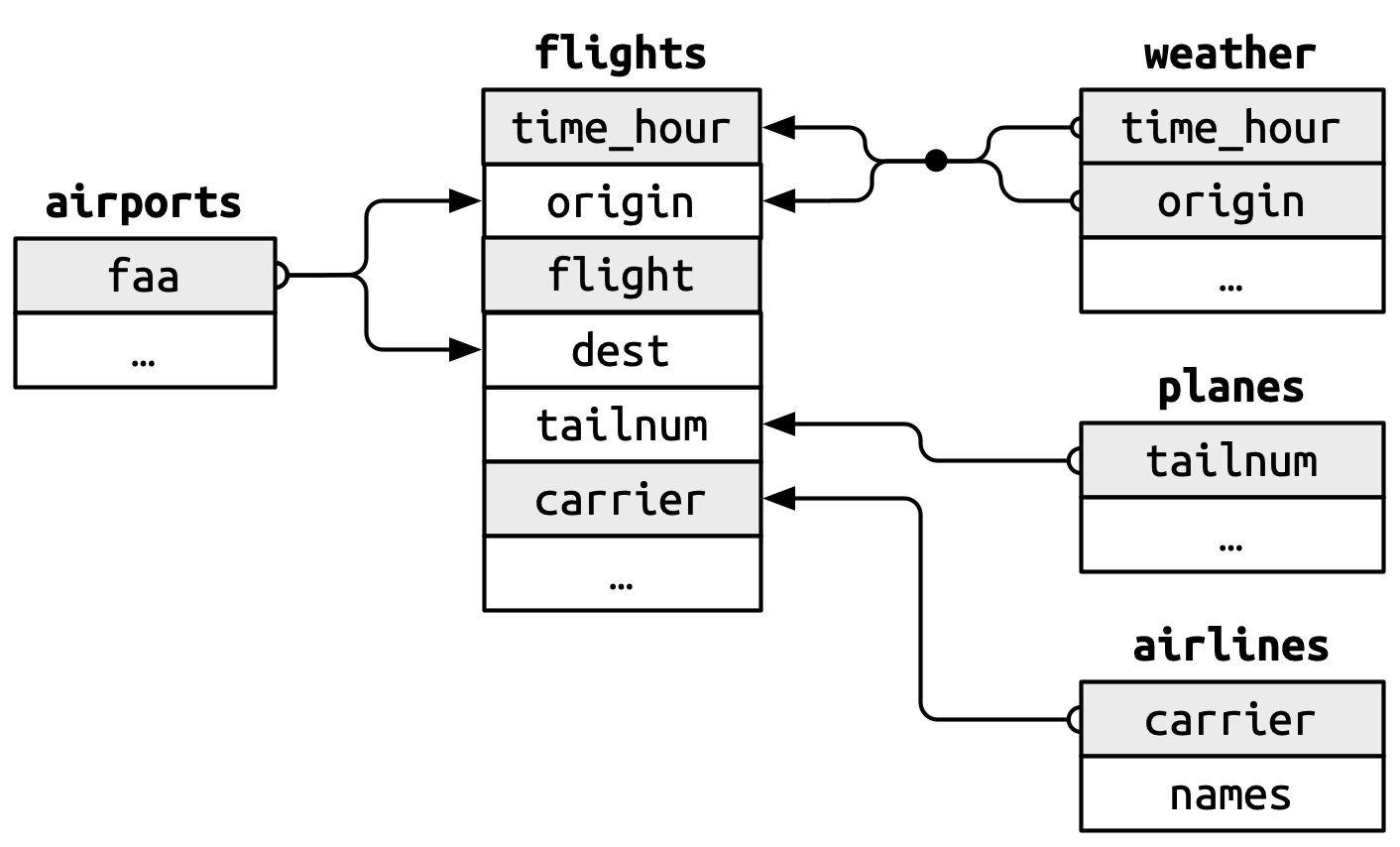{fig-align="center"}
::: {.incremental}
* `flights$origin` --> `airports$faa`
* `flights$dest` --> `airports$faa`
* `flights$origin`-`flights$time_hour` --> `weather$origin`-`weather$time_hour`.
* `flights$tailnum` --> `planes$tailnum`
* `flights$carrier` --> `airlines$carrier`
:::
## Checking Keys
A nice feature of these data are that the primary and foreign keys have the same name and almost every variable name used across multiple tables has the same meaning.^[With the exception of `year`: it means year of departure in `flights` and year of manufacture in `planes`. ] This isn't always the case!^[We'll cover how to handle this shortly.]
. . .
It is good practice to make sure your primary keys actually uniquely identify an observation and that they don't have any missing values.
. . .
```{r}
#| output-location: fragment
planes |>
count(tailnum) |> # <1>
filter(n > 1) # <1>
```
1. If your primary keys uniquely identify each observation you'll get an empty tibble in return.
. . .
```{r}
planes |>
filter(is.na(tailnum)) # <2>
```
2. If none of your primary keys are missing you'll get an empty tibble in return here too.
## Surrogate Keys
Sometimes you'll want to create an index of your observations to serve as a surrogate key because the compound primary key is not particularly easy to reference.
. . .
For example, our `flights` dataset has three variables that uniquely identify each observation: `time_hour`, `carrier`, `flight`.
. . .
```{r}
#| output-location: fragment
flights2 <- flights |>
mutate(id = row_number(), .before = 1) # <1>
flights2
```
1. `row_number()` simply specifies the row number of the data frame.
## Basic (Equi-) Joins
All join functions have the same basic interface: they take a **pair** of data frames and return **one** data frame.
. . .
The order of the rows and columns is primarily going to be determined by the first data frame.
. . .
`dplyr` has two types of joins: *mutating* and *filtering.*
:::: {.columns}
::: {.column width="50%"}
::: {.fragment}
#### Mutating Joins
Add new variables to one data frame from matching observations from another data frame.
* `left_join()`
* `right_join()`
* `inner_join()`
* `full_join()`
:::
:::
::: {.column width="50%"}
::: {.fragment}
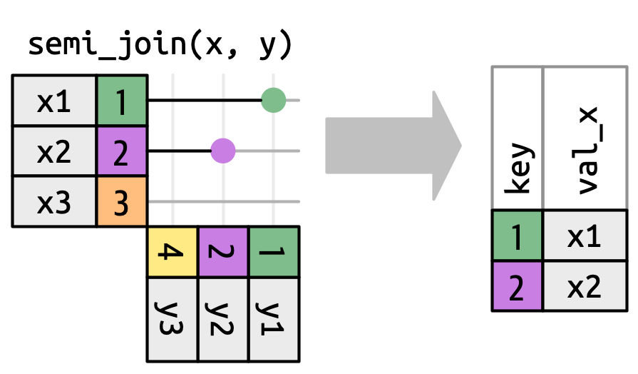
#### Filtering Joins
Filter observations from one data frame based on whether or not they match an observation in another data frame.
* `semi_join()`
* `anti-join()`
:::
:::
::::
## `Mutating Joins`
:::: {.columns}
::: {.column width="50%"}
::: {.fragment}
:::
:::
::: {.column width="50%"}
::: {.fragment}
:::
:::
::::
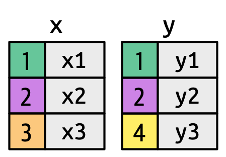
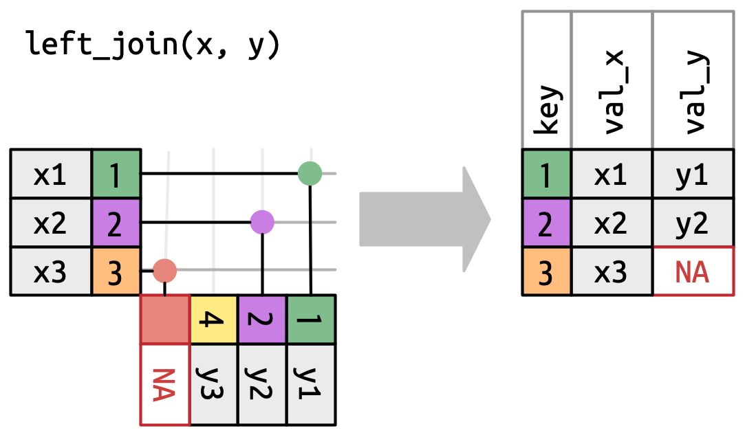
## `left_join()`
{fig-align="center"}
::: {.r-stack}
::: {.incremental}
[The most common type of join]{.fragment .fade-in-then-out fragment-index=1 .absolute top=0 right=0}
[Appends columns from `y` to `x` by the rows in `x` \
(`NA` added if there is nothing from `y`)]{.fragment fragment-index=2 .absolute top=0 right=0}
[**Natural join**: when all variables that appear in both datasets are used as the join key. \
\
*If the `join_by()` argument is not specified, `left_join()` will automatically join by all columns that have names and values in common.*]{.fragment fragment-index=3 .absolute bottom=-225 right=0 style="font-size: 80%;" width="500" height="400"}
:::
:::
## `left_join` in `nycflights13`
```{r}
flights2 <- flights |>
select(year, time_hour, origin, dest, tailnum, carrier)
```
With only the pertinent variables from the `flights` dataset, we can see how a `left_join` works with the `airlines` dataset.
```{r}
#| output-location: fragment
#| message: true
flights2 |>
left_join(y = airlines) # <1>
```
1. The `airlines` dataset has variables `carrier` and `name`
## Different variable meanings
```{r}
#| output-location: fragment
#| message: true
flights2 |>
left_join(planes) # <1>
```
1. The `planes` dataset has variables `tailnum`, `year`, `type`, `manufacturer`, `model`, `engines`, `seats`, `speed`, and `engine`
\
[When we try to do this, however, we get a bunch of `NA`s. Why?]{.fragment .fade-in-then-out}
::: aside
[*Join is trying to use tailnum and year as a compound key.* While both datasets have `year` as a variable, they mean **different** things. Therefore, we need to be explicit here about what to join by. ]{.fragment}
:::
## Different variable meanings
```{r}
#| output-location: fragment
flights2 |>
left_join(y = planes, by = join_by(tailnum)) # <1>
```
1. `join_by(tailnum)` is short for `join_by(tailnum == tailnum)` making these types of basic joins equi joins.
::: aside
[When you have the same variable name but they mean different things you can specify a particular suffix with the `suffix` argument in the `_join` function. By default the suffix will be `.x` for the variable from the first dataset and `.y` for the variable from the second dataset.]{.fragment}
:::
## Different variable names
If you have keys that have the same meaning (values) but are named different things in their respective datasets you'd also specify that with `join_by()`
. . .
```{r}
#| output-location: fragment
flights2 |>
left_join(airports, join_by(dest == faa)) # <1>
```
1. `by = c("dest" = "faa")` was the former syntax for this and you still might see that in older code. You can specify multiple `join_by`s by simply separating the conditional statements with `,` (i.e. `join_by(x == y, a == b)`).
::: aside
[This will match `dest` to `faa` for the join and then drop `faa`.]{.fragment}
:::
## Different variable names
You can request `dplyr` to keep both keys with `keep = TRUE` argument.
. . .
```{r}
#| output-location: fragment
flights2 |>
left_join(airports, join_by(dest == faa), keep = TRUE)
```
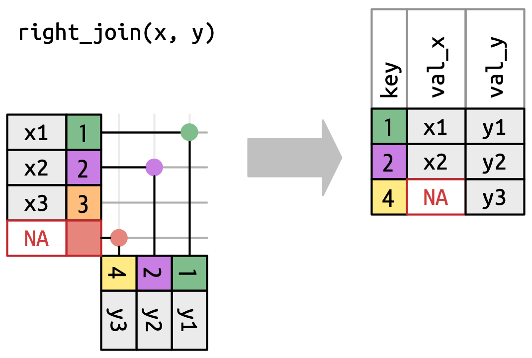
## `right_join()`
{fig-align="center"}
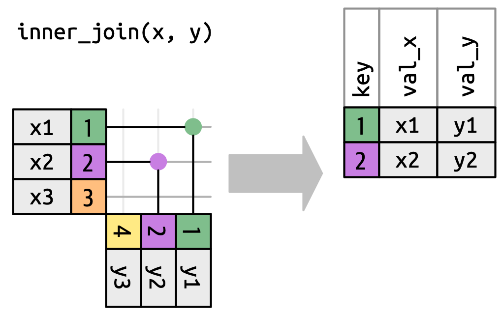
## `inner_join()`
{fig-align="center"}
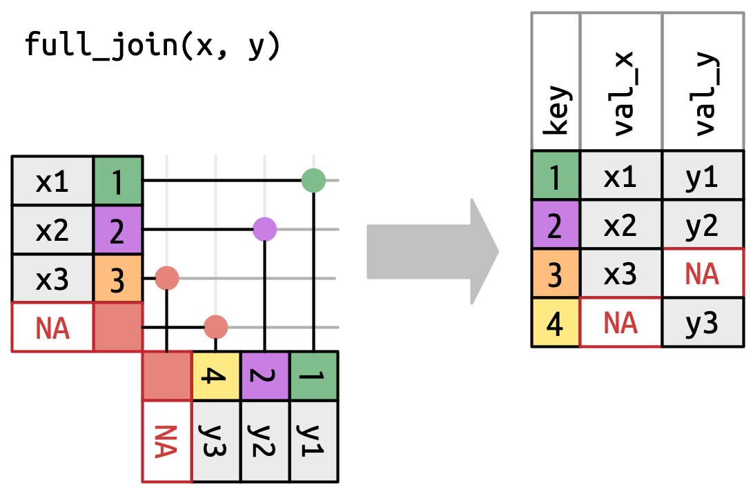
## `full_join()`
{fig-align="center"}
## `Filtering Joins`
:::: {.columns}
::: {.column width="50%"}
::: {.fragment}

:::
:::
::: {.column width="50%"}
::: {.fragment}

:::
:::
::::
## `semi_join()`
{fig-align="center"}
## `semi_join()` in `nycflights13`
We could use a semi-join to filter the airports dataset to show just the origin airports.
. . .
```{r}
#| output-location: fragment
airports |>
semi_join(flights2, join_by(faa == origin))
```
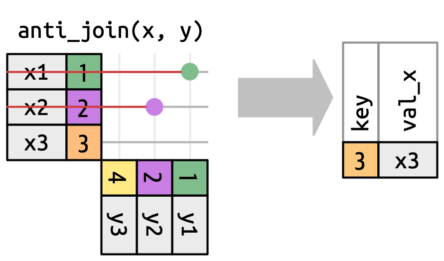
## `anti_join()`
{fig-align="center"}
## `anti_join()` in `nycflights13`
We can find rows that are missing from airports by looking for flights that don’t have a matching destination airport.
. . .
```{r}
#| output-location: fragment
airports |>
anti_join(flights2, join_by(faa == origin))
```
::: aside
[This type of join is useful for finding missing values that are implicit in the data (i.e. `NA`s that don't show up in the data but only exist as an absence.)]{.fragment}
:::
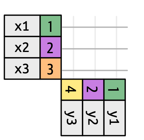
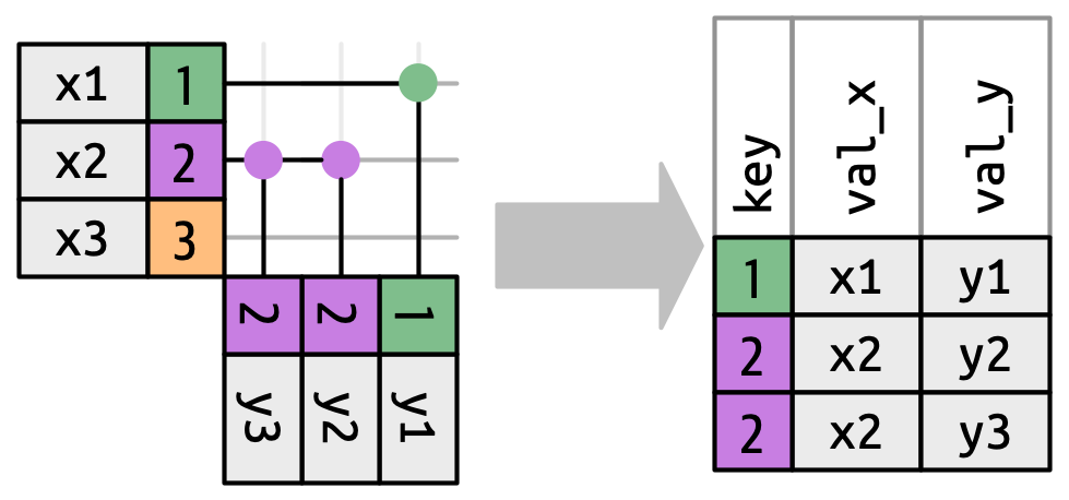
## More Than One Match
{fig-align="center"}
. . .
There are three possible outcomes for a row in x:
::: {.incremental}
* If it doesn’t match anything, it’s dropped.
* If it matches 1 row in `y`, it’s preserved.
* If it matches more than 1 row in ` y`, it’s duplicated once for each match.
:::
. . .
What happens if we match on more than one row?
## More Than One Match
```{r}
#| output-location: fragment
#| warning: true
df1 <- tibble(key = c(1, 2, 2), val_x = c("x1", "x2", "x3"))
df2 <- tibble(key = c(1, 2, 2), val_y = c("y1", "y2", "y3"))
df1 |>
inner_join(df2, join_by(key))
```
::: {.aside}
::: {.r-stack}
[If you are doing this deliberately, you can set `relationship = "many-to-many"`, as the warning suggests.]{.fragment .fade-in-then-out}
[Note: Given their nature, *filtering* joins never duplicate rows like mutating joins do. They will only ever return a subset of the datasets.]{.fragment}
:::
:::
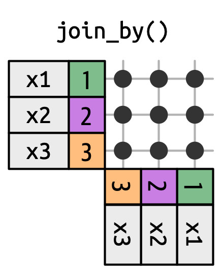
## Non-Equi Joins
The joins we've discussed thus far have all been equi-joins, where the rows match if the x key equals the y key. But you can also specify other types of relationships.
. . .
`dplyr` has four different types of non-equi joins:
. . .
:::: {.columns}
::: {.column width="50%"}
* **Cross joins** match every pair of rows.
:::
::: {.column width="50%"}
{width=25% .absolute top=150 right=150}
:::
::::
::: aside
[Cross joins, aka self-joins, are useful when generating permutations (e.g. creating every possible combination of values). This comes in handy when creating datasets of predicted probabilities for plotting in ggplot.]{.fragment}
:::
## Non-Equi Joins
The joins we've discussed thus far have all been equi-joins, where the rows match if the x key equals the y key. But you can also specify other types of relationships.
`dplyr` has four different types of non-equi joins:
:::: {.columns}
::: {.column width="50%"}
* **Cross joins** match every pair of rows.
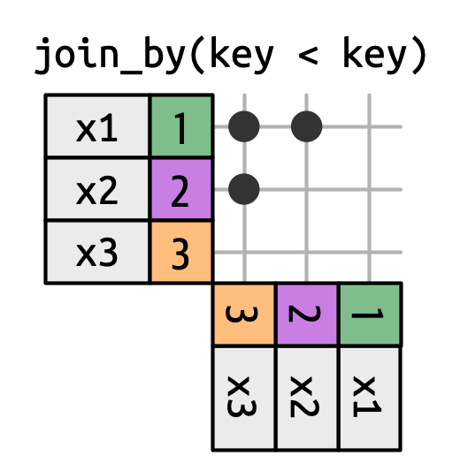
* **Inequality joins** use <, <=, >, and >= instead of ==.
* **Overlap joins** are a special type of inequality join designed to work with ranges^[Overlap joins provide three helpers that use inequality joins to make it easier to work with intervals: `between()`, `within()`, `overlaps()`. Read more about their functionality and specifications [here](https://dplyr.tidyverse.org/reference/join_by.html?q=within#overlap-joins).].
:::
::: {.column width="50%"}
{width=30% .absolute top=158 right=120}
:::
::::
::: aside
Inequality joins can be used to restrict the cross join so that instead of generating all permutations, we generate all combinations.
:::
## Non-Equi Joins
The joins we've discussed thus far have all been equi-joins, where the rows match if the x key equals the y key. But you can also specify other types of relationships.
`dplyr` has four different types of non-equi joins:
:::: {.columns}
::: {.column width="50%"}
* **Cross joins** match every pair of rows.
* **Inequality joins** use <, <=, >, and >= instead of ==.
* **Overlap joins** are a special type of inequality join designed to work with ranges.
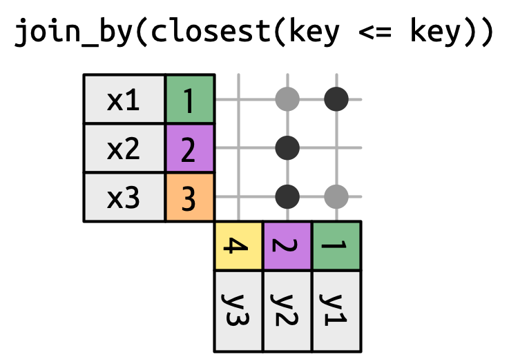
* **Rolling joins** are similar to inequality joins but only find the closest match.
:::
::: {.column width="50%"}
{width=42% .absolute top=155 right=35}
:::
::::
::: aside
Rolling joins are a special type of inequality join where instead of getting every row that satisfies the inequality, you get just the closest row. You can turn any inequality join into a rolling join by adding closest().
:::
# Homework{.section-title background-color="#1e4655"}
## {data-menu-title="Homework 4" background-iframe="https://vsass.github.io/CSSS508/Homework/HW4/homework4.html" background-interactive=TRUE}