---
execute: 
  echo: true
  message: false
  warning: false
  fig-format: "svg"
format: 
  revealjs:
    highlight-style: a11y-dark  
    reference-location: margin
    theme: lecture_styles.scss
    slide-number: true
    code-link: true
    chalkboard: true
    incremental: false 
    smaller: true
    preview-links: true
    code-line-numbers: true
    history: false
    progress: true
    link-external-icon: true
    code-annotations: hover
    pointer:
      color: "#b18eb1"
revealjs-plugins:
  - pointer
---

```{r}
#| echo: false
#| cache: false
require(downlit)
require(xml2)
require(tidyverse)

knitr::opts_chunk$set(
  comment = ">")
```

## {#title-slide data-menu-title="Data Structures & Types" background="#1e4655" background-image="../../images/csss-logo.png" background-position="center top 5%" background-size="50%"}


[Data Structures & Types]{.custom-title}

[CS&SS 508 • Lecture 6]{.custom-subtitle}

[{{< var lectures.six >}}]{.custom-subtitle2}

[Victoria Sass]{.custom-subtitle3}

# Roadmap{.section-title background-color="#99a486"}

---

:::: {.columns}

::: {.column width="50%"}

<br>

### Last time, we learned:

* Importing and Exporting Data
* Tidying and Reshaping Data
* Types of Data
  * Working with Factors
  * Wrangling Date/Date-Time Data
:::

::: {.column width="50%"}

<br> 

::: {.fragment}
### Today, we will cover:

* Types of Data
  * Numbers
  * Missing Values
* Data Structures
  * Vectors
  * Matrices
  * Lists

:::

:::

::::

. . . 

This week we start getting more into the weeds of programming in `R`. 

. . . 

These skills will help you understand some of `R`'s quirks, how to troubleshoot errors when they arise, and how to write more efficient and automated code that does a lot of work for you! 

## Data types in `R`

Returning, once again, to our list of data types in `R`: 

. . . 

* Logicals
* Factors
* Date/Date-time
* Numbers
* Missing Values
* Strings

## Data types in `R`

Returning, once again, to our list of data types in `R`: 

* <span style="color:#af7aa1">Logicals<span>
* <span style="color:#af7aa1">Factors<span>
* Date/Date-time
* Numbers
* Missing Values
* Strings

![](images/logicals_factors.png){.absolute top=100 right=0 left=250 width="900" height="600"}

## Data types in `R`

Returning, once again, to our list of data types in `R`: 

* Logicals
* Factors
* <span style="color:#af7aa1">Date/Date-time<span>
* Numbers
* Missing Values
* Strings

![](images/lubridate.png){.absolute top=75 right=0 left=200}

## Data types in `R`

Returning, once again, to our list of data types in `R`: 

* ~~Logicals~~
* ~~Factors~~
* ~~Date/Date-time~~
* <span style="color:#e15759">Numbers<span>
* <span style="color:#e15759">Missing Values</span>
* Strings

# Numbers{.section-title background-color="#99a486"}

## Numbers, Two Ways

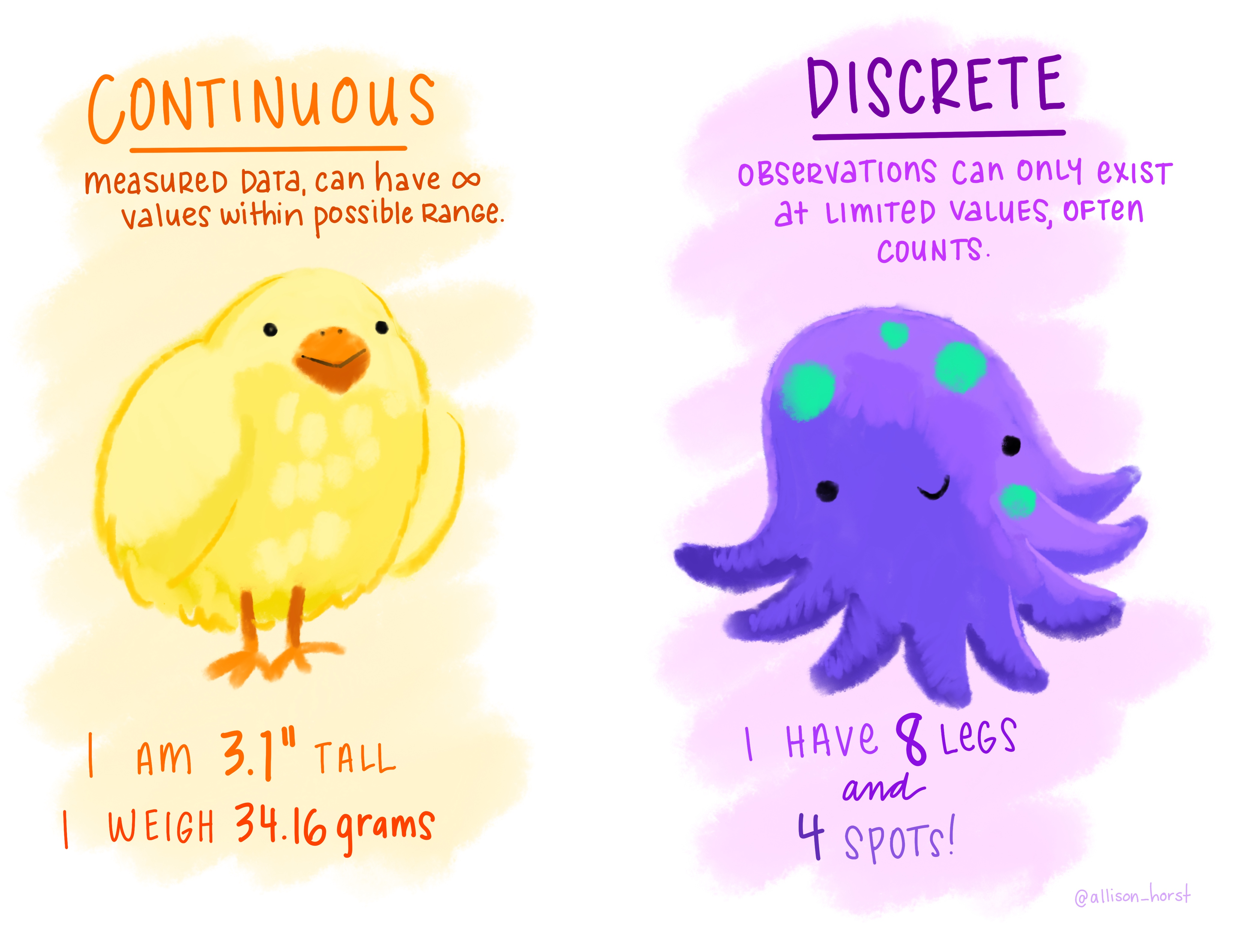
`R` has two types of numeric variables: `double` and `integer`. 

. . . 

![](images/numbers.png){fig-align="center" width=70% height=70%}

## Numbers Coded as Character Strings

Oftentimes numerical data is coded as a string so you'll need to use the appropriate parsing function to read it in in the correct form. 

. . . 

```{r}
parse_integer(c("1", "2", "3"))
parse_double(c("1", "2", "3.123"))
```

. . . 

<br>

If you have values with extraneous non-numerical text you want to ignore there's a separate function for that.

. . . 

```{r}
parse_number(c("USD 3,513", "59%", "$1,123,456.00"))
```

## `count()`

A very useful and common exploratory data analysis tool is to check the relative sums of different categories of a variable. That's what `count()` is for!

. . . 

```{r}
library(nycflights13)
data(flights)

flights |> count(origin) # <1> 
```
1. Add the argument `sort = TRUE` to see the most common values first (i.e. arranged in descending order).
. . . 

This is functionally the same as grouping and summarizing with `n()`.

. . . 

```{r}
flights |> 
  summarise(n= n(), # <2>
            .by = origin) # <3>
```
2. `n()` is a special summary function that doesn’t take any arguments and instead accesses information about the “current” group. This means that it only works inside dplyr verbs. 
3. You can do this longer version if you also want to compute other summaries simultaneously. 

## `n_distinct()`

Use this function if you want the count the number of distinct (unique) values of one or more variables. 

. . . 

Say we're interested in which destinations are served by the most carriers:

```{r}
flights |> 
  summarize(carriers = n_distinct(carrier), 
            .by = dest) |> 
  arrange(desc(carriers))
```

## Weighted Counts

A weighted count is simply a grouped sum, therefore `count` has a `wt` argument to allow for the shorthand. 

. . . 

:::: {.columns}

::: {.column width="45%"}

How many miles did each plane fly? 

```{r}
flights |> 
  summarize(miles = sum(distance), 
            .by = tailnum)
```

:::

::: {.column width="55%"}

::: {.fragment}
This is equivalent to: 

```{r}
flights |> count(tailnum, wt = distance) 
```
:::

:::

::::

## Other Useful Arithmetic Functions

```{r}
#| echo: false
df <- tribble(
  ~x, ~y,
  1,  3,
  5,  2,
  7, NA,
)
```

In addition to the standards (`+`, `-`, `/`, `*`, `^`), `R` has many other useful arithmetic functions. 

. . . 

**Pairwise min/max**

```{r}
df
```

```{r}
df |> 
  mutate(
    min = pmin(x, y, na.rm = TRUE), # <6>
    max = pmax(x, y, na.rm = TRUE) # <7>
  )
```
6. `pmin()` returns the smallest value in each row. `min()`, by contrast, finds the smallest observation given a number of rows.
7. `pmax()` returns the largest value in each row. `max()`, by contrast, finds the largest observation given a number of rows.

## Other Useful Arithmetic Functions

**Modular arithmetic**

```{r}
1:10 %/% 3 # <8>
```
8. Computes integer division. 

```{r}
1:10 %% 3 # <9>
```
9. Computes the remainder. 

. . . 

We can see how this can be useful in our `flights` data which has curiously stored time: 

```{r}
flights |> mutate(hour = sched_dep_time %/% 100,
                  minute = sched_dep_time %% 100,
                  .keep = "used")
```

## Other Useful Arithmetic Functions

**Logarithms**^[An incredibly useful transformation for dealing with data that ranges across multiple orders of magnitude and converting exponential growth to linear growth.]

```{r}
log(c(2.718282, 7.389056, 20.085537)) # <10> 
```
10. Inverse is `exp()`
```{r}
log2(c(2, 4, 8)) # <11>
```
11. Easy to interpret because a difference of 1 on the log scale corresponds to doubling on the original scale and a difference of -1 corresponds to halving. Inverse is `2^`. 
```{r}
log10(c(10, 100, 1000)) # <12>
```
12. Easy to back-transform because everything is on the order of 10. Inverse is `10^`. 

## Other Useful Arithmetic Functions

**Cumulative and Rolling Aggregates**

Base `R` provides `cumsum()`, `cumprod()`, `cummin()`, `cummax()` for running, or cumulative, sums, products, mins and maxes. `dplyr` provides `cummean()` for cumulative means.

. . . 

```{r}
1:15
```

```{r}
cumsum(1:15) # <13>
```
13. `cumsum()` is the most common in practice.

. . . 

For complex rolling/sliding aggregates, check out the [`slidr` package](https://slider.r-lib.org/index.html). 

## Other Useful Arithmetic Functions

**Numeric Ranges**

```{r}
x <- c(1, 2, 5, 10, 15, 20)
cut(x, breaks = c(0, 5, 10, 15, 20)) # <14> 
```
14. `cut()` breaks up (aka bins) a numeric vector into discrete buckets

. . . 

```{r}
cut(x, breaks = c(0, 5, 10, 100)) # <15>
```
15. The bins don't have to be the same size.

. . . 

```{r}
cut(x, 
  breaks = c(0, 5, 10, 15, 20), 
  labels = c("sm", "md", "lg", "xl") # <16>
)
```
16. You can optionally supply your own labels. Note that there should be one less labels than breaks.

. . . 

```{r}
y <- c(NA, -10, 5, 10, 30) # <17>
cut(y, breaks = c(0, 5, 10, 15, 20))
```
17. Any values outside of the range of the breaks will become `NA`.

## Rounding 

`round()` allows us to round to a certain decimal place. Without specifying an argument for the `digits` argument it will round to the nearest integer. 

. . . 

```{r}
round(pi)
round(pi, digits = 2)
```

. . . 

Using negative integers in the `digits` argument allows you to round on the left-hand side of the decimal place. 

```{r}
round(39472, digits = -1)
round(39472, digits = -2)
round(39472, digits = -3)
```

## Rounding 

What's going on here?

```{r}
round(c(1.5, 2.5)) 
```

. . . 

`round()` uses what’s known as “round half to even” or Banker’s rounding: if a number is half way between two integers, it will be rounded to the even integer. This is a good strategy because it keeps the rounding **unbiased**: half of all 0.5s are rounded up, and half are rounded down.

. . . 

<br>

`floor()` and `ceiling()` are also useful rounding shortcuts.

```{r}
floor(123.456) # <18>
```
18. Always rounds down.
```{r}
ceiling(123.456) # <19>
```
19. Always rounds up. 

## Summary Functions 

. . . 

**Central Tendency**

```{r}
x <- sample(1:500, size = 100, replace = TRUE) # <20>
mean(x)
```
20. `sample()` takes a vector of data, and samples `size` elements from it, with replacement if `replace` equals `TRUE`. 
```{r}
median(x)
```

```{r}
quantile(x, .95) # <21>
```
21. A generalization of the median: `quantile(x, 0.95)` will find the value that’s greater than 95% of the values; `quantile(x, 0.5)` is equivalent to the median.

## Summary Functions 

**Measures of Spread/Variation**

```{r}
min(x)
max(x)
range(x)
```

```{r}
IQR(x) # <22>
```
22. Equivalent to `quantile(x, 0.75) - quantile(x, 0.25)` and gives you the range that contains the middle 50% of the data.

```{r}
var(x) # <23>
```
23. $$s^2 = \frac{\sum(x_i-\overline{x})^2}{n-1}$$ 

```{r}
sd(x) # <24>
```
24. $$s = \sqrt{\frac{\sum(x_i-\overline{x})^2}{n-1}}$$

## Common Numerical Manipulations

These formulas can be used in a summary call but are also useful with `mutate()`, particularly if being applied to grouped data. 

. . . 

```{r}
#| eval: false
x / sum(x) # <19> 
(x - mean(x)) / sd(x) # <20>
(x - min(x)) / (max(x) - min(x)) # <21>
x / first(x) # <22>
```
19. Calculates the proportion of a total.
20. Computes a Z-score (standardized to mean 0 and sd 1). 
21. Standardizes to range [0, 1].
22. Computes an index based on the first observation.

## Summary Functions 

**Positions**

```{r}
first(x)
last(x)
nth(x, n = 77)
```

. . . 

<br>

These are all really helpful but is there a *good* summary descriptive statistics function?

# {data-menu-title="`skimr`" background-image="images/skimr_logo.png" background-size="contain" background-position="center" .section-title background-color="#1e4655"}

## Basic summary statistics

. . . 

```{r}
summary(iris)
```

## Better summary statistics <span style="color:#99a486">{{< fa scroll >}}</span> {.scrollable} 

A basic example:

```{r}
library(skimr)
skim(iris)
```

## Better summary statistics <span style="color:#99a486">{{< fa scroll >}}</span> {.scrollable} 

A more complex example: 

```{r}
skim(starwars)
```

## `skim` function

Highlights of this summary statistics function: 

::: {.incremental}
- provides a larger set of statistics than `summary()` including number missing, complete, n, sd, histogram for numeric data
- presentation is in a compact, organized format
- reports each data type separately
- handles a wide range of data classes including dates, logicals, strings, lists and more
- can be used with `summary()` for an overall summary of the data (w/o specifics about columns)
- individual columns can be selected for a summary of only a subset of the data
- handles grouped data
- behaves nicely in pipelines
- produces knitted results for documents
- easily and highly customizable (i.e. specify your own statistics and classes)
:::

# Missing Values{.section-title background-color="#99a486"}

## Explicit Missing Values

. . . 

> *An explicit missing value is the presence of an absence.*

. . . 

In other words, an explicit missing value is one in which you see an `NA`. 

. . . 

Depending on the reason for its missingness, there are different ways to deal with `NA`s.

. . . 

**Data Entry Shorthand**

If your data were entered by hand and `NA`s merely represent a value being carried forward from the last entry then you can use `fill()` to help complete your data.

:::: {.columns}

::: {.column width="50%"}
::: {.fragment}
```{r}
treatment <- tribble(
  ~person,           ~treatment, ~response,
  "Derrick Whitmore", 1,         7,
  NA,                 2,         10,
  "Katherine Burke",  3,         NA,
  NA,                 1,         4
)
```
:::
:::

::: {.column width="50%"}
::: {.fragment}
```{r}
treatment |>
  fill(everything()) # <1> 
```
1. `fill()` takes one or more variables (in this case `everything()`, which means all variables), and by default fills them in downwards. If you have a different issue you can change the `.direction` argument to `"up"`,`"downup"`, or `"updown"`. 
:::
:::
::::

## Explicit Missing Values

**Represent A Fixed Value**

Other times an `NA` represents some fixed value, usually `0`. 

. . . 

```{r}
x <- c(1, 4, 5, 7, NA)
coalesce(x, 0) # <2> 
```
2. `coalesce()` in the `dplyr` package takes a vector as the first argument and will replace any missing values with the value provided in the second argument. 

. . . 

<br>

**Represented By a Fixed Value**

If the opposite issue occurs (i.e. a value is actually an `NA`), try specifying that to the `na` argument of your `readr` data import function. Otherwise, use `na_if()` from `dplyr`. 

```{r}
x <- c(1, 4, 5, 7, -99)
na_if(x, -99)
```

## Explicit Missing Values

**`NaN`s**

A special sub-type of missing value is an `NaN`, or `N`ot `a` `N`umber. 

. . . 

These generally behave similar to `NA`s and are likely the result of a mathematical operation that has an indeterminate result:

```{r}
0 / 0 
0 * Inf
Inf - Inf
sqrt(-1)
```

. . . 

If you need to explicitly identify an `NaN` you can use `is.nan()`. 

## Implicit `NA`s

> *An implicit missing value is the absence of a presence.*

. . . 

We've seen a couple of ways that implicit `NA`s can be made explicit in previous lectures: `pivoting` and `joining`. 

. . . 

```{r}
#| echo: false
stocks <- tibble(
  year  = c(2020, 2020, 2020, 2020, 2021, 2021, 2021),
  qtr   = c(   1,    2,    3,    4,    2,   3,    4),
  price = c(1.88, 0.59, 0.35, 0.89, 0.34, 0.17, 2.66)
)
```

. . . 

For example, if we *really* look at the dataset below, we can see that there are missing values that don't appear as `NA` merely due to the current structure of the data.

```{r}
stocks
```

## Implicit `NA`s

`tidyr::complete()` allows you to generate explicit missing values by providing a set of variables that define the combination of rows that should exist.

:::: {.columns}

::: {.column width="35%"}
::: {.fragment}
```{r}
stocks |>
  complete(year, qtr)
```
:::
:::

::: {.column width="65%"}
::: {.fragment}
```{r}
stocks |>
  complete(year, qtr, fill = list(price = 0.93))
```
:::
:::

::::

::: aside
The `fill` argument of `complete` only allows you to supply 1 value per variable. If you have more than one value to fill, use `complete` to create the data structure you need, and `case_when` to replace `NA`s would be the most straightforward approach.
:::

## Missing Factor Levels

. . . 

The last type of missingness is a theoretical level of a factor that doesn't have any observations. 

```{r}
#| echo: false
health <- tibble(
  name   = c("Ikaia", "Oletta", "Leriah", "Dashay", "Tresaun"),
  smoker = factor(c("no", "no", "no", "no", "no"), levels = c("yes", "no")),
  age    = c(34, 88, 75, 47, 56),
)
```

. . . 

For instance, we have this `health` dataset and we're interested in smokers:

:::: {.columns}

::: {.column width="45%"}
::: {.fragment}
```{r}
health
```
:::
::: {.fragment}
```{r}
health |> count(smoker)
```
:::
:::

::: {.column width="55%"}

::: {.fragment}
```{r}
levels(health$smoker) # <3> 
```
3. This dataset only contains non-smokers, but we know that smokers exist; the group of smokers is simply empty. 
:::

::: {.fragment}

<br>
<br>
<br>
<br>

```{r}
health |> count(smoker, .drop = FALSE) # <4>
```
4. We can request `count()` to keep all the groups, even those not seen in the data by using `.drop = FALSE`.
:::

:::

::::


## Missing Factors in Plots

This sample principle applies when visualizing a factor variable, which will automatically drop levels that don’t have any values. Use `drop_values = FALSE` in the appropriate scale to display implicit `NA`s. 

. . . 

:::: {.columns}

::: {.column width="50%"}
```{r}
ggplot(health, aes(x = smoker)) +
  geom_bar() +
  scale_x_discrete() + 
  theme_classic(base_size = 22)
```

:::

::: {.column width="50%"}
::: {.fragment}

```{r}
#| code-line-numbers: "3"
ggplot(health, aes(x = smoker)) +
  geom_bar() +
  scale_x_discrete(drop = FALSE) + 
  theme_classic(base_size = 22)
```
:::
:::

::::

## Testing Data Types

There are also functions to **test** for certain data types:

. . . 

```{r}
is.numeric(5)
is.character("A")
is.logical(TRUE)
is.infinite(-Inf)
is.na(NA)
is.nan(NaN)
```

## Going deeper into the abyss (aka `NA`s)

![](images/naniar_horst.png){fig-align="center"}

::: aside
*Artwork by [@allison_horst](https://twitter.com/allison_horst)*
:::

## Going deeper into the abyss (aka `NA`s)

A lot has been written about `NA`s and if they are a feature of your data you're likely going to have to spend a great deal of time thinking about how they arose^[Missing Completely at Random? Missing at Random? Missing Not at Random? Read more about the differences [here](https://www.ncbi.nlm.nih.gov/books/NBK493614/).] and if/how they bias your data. 

. . . 

:::: {.columns}

::: {.column width="50%"}
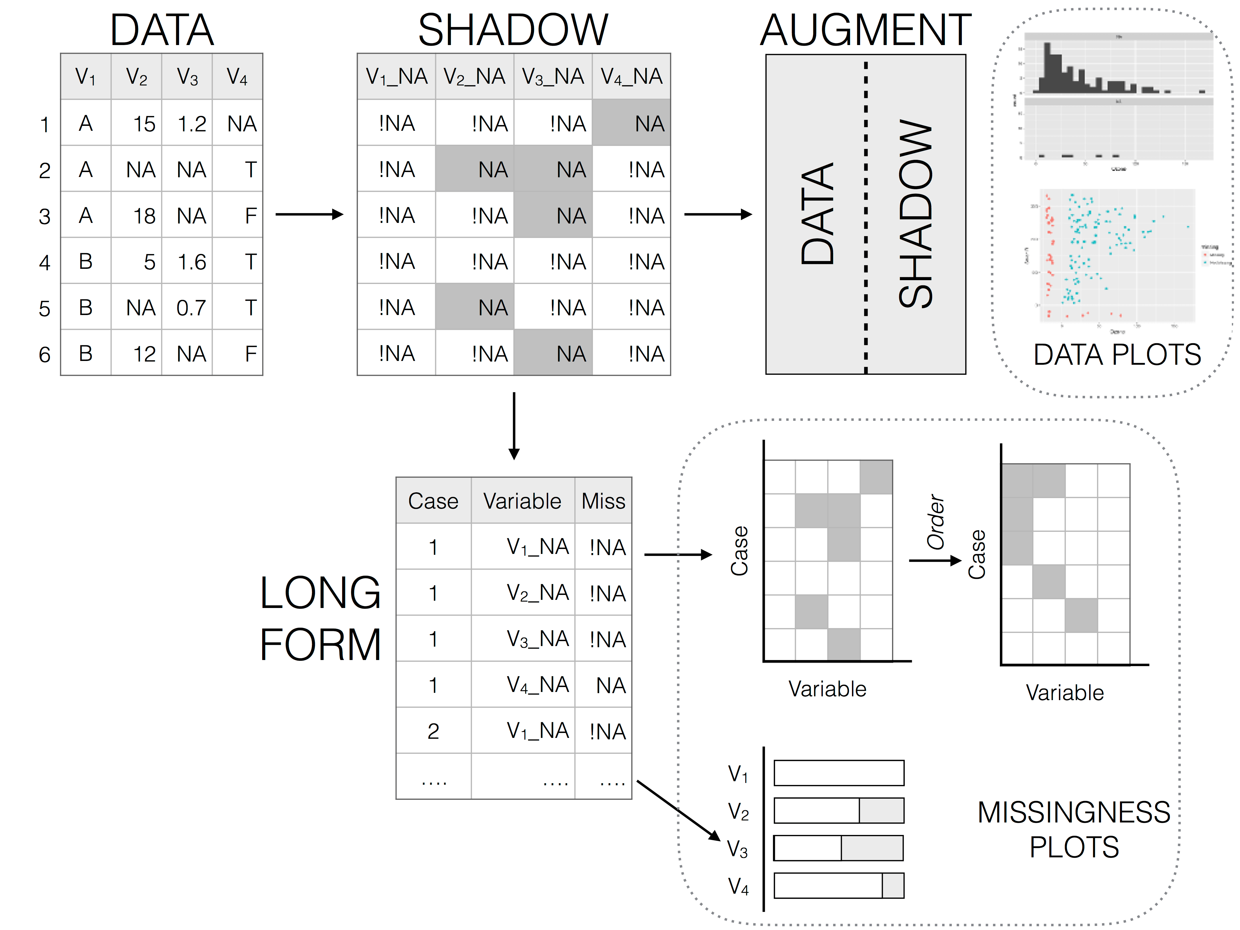
The best package for really exploring your `NA`s is [`naniar`](https://naniar.njtierney.com/), which provides tidyverse-style syntax for summarizing, visualizing, and manipulating missing data. 

<br>

It provides the following for missing data:

::: {.incremental}
- a special data structure
- shorthand and numerical summaries (in variables and cases)
- visualizations
:::
:::

::: {.column width="50%"}
![](images/naniar_logo.png){fig-align="center" width=60%}
:::

::::

## `naniar` examples

. . .

![](images/missingness-data-structures.png){fig-align="center" width=80%}

::: aside
See more [here](https://naniar.njtierney.com/articles/naniar.html).
:::

## `visdat` example

```{r} 
#| fig-height: 5
#| fig-format: png
#| fig-align: center
#| output-location: fragment
library(visdat)
vis_dat(airquality)
```

::: aside
You can read more about this package and its functionality [here](https://cran.r-project.org/web/packages/visdat/vignettes/using_visdat.html). For an tidy-style approach for imputing missing values check out the [`simputation`](https://cran.r-project.org/web/packages/simputation/vignettes/intro.html) package.
::: 

# Break!{.section-title background-color="#1e4655"}

# Vectors{.section-title background-color="#99a486"}

## Making Vectors

In R, we call a set of values of the same type a **vector**. We can create vectors using the `c()` function ("c" for `c`ombine or `c`oncatenate).

```{r}
c(1, 3, 7, -0.5)
```

. . . 

Vectors have one dimension: **length**

```{r}
length(c(1, 3, 7, -0.5))
```

. . . 

All elements of a vector are the same type (e.g. numeric or character)!

. . . 

Character data is the lowest denomination so anything mixed with it will be converted to a character. 

## Generating Numeric Vectors

There are shortcuts for generating numeric vectors:

```{r}
1:10
```

. . . 

```{r}
seq(-3, 6, by = 1.75) # <1>
```
1. Sequence from -3 to 6, increments of 1.75

. . . 

```{r}
rep(c(0, 1), times = 3) # <2>
rep(c(0, 1), each = 3) # <3>
rep(c(0, 1), length.out = 3) # <4>
```
2. Repeat `c(0, 1)` 3 times.
3. Repeat each element 3 times.
4. Repeat `c(0, 1)` until the length of the final vector is 3. 

. . . 

You can also assign values to a vector using Base `R` indexing rules. 

. . . 

```{r}
x <- c(3, 6, 2, 9, 5)
x[6] <- 8
x
x[c(7, 8)] <- c(9, 9)
x
```

## Element-wise Vector Math

When doing arithmetic operations on vectors, R handles these *element-wise*:

```{r}
c(1, 2, 3) + c(4, 5, 6)
```

```{r}
c(1, 2, 3, 4)^3 # <5> 
```
5. Exponentiation is carried out using the `^` operator.

. . . 

Other common operations: `*`, `/`, `exp()` = $e^x$, `log()` = $\log_e(x)$

## Recycling Rules

`R` handles mismatched lengths of vectors by recycling, or repeating, the short vector.

. . . 

```{r}
x <- c(1, 2, 10, 20)
x / 5 # <6> 
```
6. This is shorthand for: `x / c(5, 5, 5, 5)`

. . . 

You generally only want to recycle scalars, or vectors the length 1. Technically, however, `R` will recycle any vector that's shorter in length (and it *won't always* give you a warning that that's what it's doing, i.e. if the longer vector is not a multiple of the shorter vector).

. . . 

```{r}
#| warning: true
x * c(1, 2)
x * c(1, 2, 3)
```

## Recycling with Logicals 

The same rules apply to logical operations which can lead to unexpected results *without warning*. 

. . . 

For example, take this code which attempts to find all flights in January and February:

```{r}
flights |> 
  filter(month == c(1, 2)) |> # <7> 
  head(5)
```
7. A common mistake is to mix up `==` with `%in%`. This code will actually find flights in odd numbered rows that departed in January and flights in even numbered rows that departed in February. Unfortunately there’s no warning because `flights` has an even number of rows. 

. . . 

To protect you from this type of silent failure, most tidyverse functions use a stricter form of recycling that only recycles single values. However, when using base `R` functions like `==`, this protection is not built in. 

## Example: Standardizing Data

Let's say we had some test scores and we wanted to put these on a standardized scale: 

$$z_i = \frac{x_i - \text{mean}(x)}{\text{SD}(x)}$$

. . . 

```{r}
x <- c(97, 68, 75, 77, 69, 81)
z <- (x - mean(x)) / sd(x)
round(z, 2)
```


## Math with Missing Values

Even one `NA` "poisons the well": You'll get `NA` out of your calculations unless you add the extra argument `na.rm = TRUE` (available in some functions):

. . . 

```{r}
vector_w_missing <- c(1, 2, NA, 4, 5, 6, NA)
mean(vector_w_missing)
mean(vector_w_missing, na.rm = TRUE)
```

## Subsetting Vectors

Recall, we can **subset** a vector in a number of ways:

* Passing a single index or vector of entries to **keep**:

```{r}
first_names <- c("Andre", "Brady", "Cecilia", "Danni", "Edgar", "Francie")
first_names[c(1, 2)]
```

. . . 

* Passing a single index or vector of entries to **drop**:

```{r}
first_names[-3]
```

. . . 

* Passing a **logical condition**:

```{r}
first_names[nchar(first_names) == 7] # <8>
```
8. `nchar()` counts the number of characters in a character string. 

. . . 

* Passing a **named vector**: 

```{r}
pet_names <- c(dog = "Lemon", cat = "Seamus")
pet_names["cat"]
```





# Matrices{.section-title background-color="#99a486"}

## Matrices: Two Dimensions

**Matrices** extend vectors to two **dimensions**: **rows** and **columns**. We can construct them directly using `matrix()`.

. . . 

R fills in a matrix column-by-column (**not** row-by-row!)

```{r}
a_matrix <- matrix(first_names, nrow = 2, ncol = 3)
a_matrix
```

. . . 

Similar to vectors, you can make assignments using Base `R` indexing methods. 

. . . 

```{r}
a_matrix[1, c(1:3)] <- c("Hakim", "Tony", "Eduardo")
a_matrix
```

. . . 

However, you can't add rows or columns to a matrix in this way. You can only reassign already-existing cell values. 

```{r}
#| error: true
a_matrix[3, c(1:3)] <- c("Lucille", "Hanif", "June")
```

## Binding Vectors

We can also make matrices by *binding* vectors together with `rbind()` (`r`ow `bind`) and `cbind()` (`c`olumn `bind`).

. . . 

```{r}
b_matrix <- rbind(c(1, 2, 3), c(4, 5, 6))
b_matrix
c_matrix <- cbind(c(1, 2), c(3, 4), c(5, 6))
c_matrix
```

## Subsetting Matrices

We subset matrices using the same methods as with vectors, except we index them with `[rows, columns]`^[Like we learned how to do with dataframes in week 3.]:

```{r}
a_matrix
```

. . . 

```{r}
a_matrix[1, 2] # <9> 
```
9. Row 1, Column 2.
```{r}
a_matrix[1, c(2,3)] # <10> 
```
10. Row 1, Columns 2 and 3. 

. . . 

We can obtain the dimensions of a matrix using `dim()`.

```{r}
dim(a_matrix)
```

## Matrices Becoming Vectors

If a matrix ends up having just one row or column after subsetting, by default `R` will make it into a vector. 

. . . 

```{r}
a_matrix[, 1] 
```

. . . 

You can prevent this behavior using `drop = FALSE`.

```{r}
a_matrix[, 1, drop = FALSE] 
```

## Matrix Data Type Warning

Matrices can contain numeric, integer, factor, character, or logical. But just like vectors, *all elements must be the same data type*.

. . . 

```{r}
bad_matrix <- cbind(1:2, c("Victoria", "Sass"))
bad_matrix
```

. . . 

In this case, everything was converted to characters!

## Matrix Dimension Names

We can access dimension names or name them ourselves:

. . . 

```{r}
rownames(bad_matrix) <- c("First", "Last")
colnames(bad_matrix) <- c("Number", "Name")
bad_matrix
```

```{r}
bad_matrix[ ,"Name", drop = FALSE] # <11>
```
11. `drop = FALSE` maintains the matrix structure; when `drop = TRUE` (the default) it will be converted to a vector. 

## Matrix Arithmetic

Matrices of the same dimensions can have math performed element-wise with the usual arithmetic operators:

. . . 

```{r}
matrix(c(2, 4, 6, 8),nrow = 2, ncol = 2) / matrix(c(2, 1, 3, 1),nrow = 2, ncol = 2)
```

## "Proper" Matrix Math

To do matrix transpositions, use `t()`.

. . . 

```{r}
c_matrix
e_matrix <- t(c_matrix)
e_matrix
```

. . . 

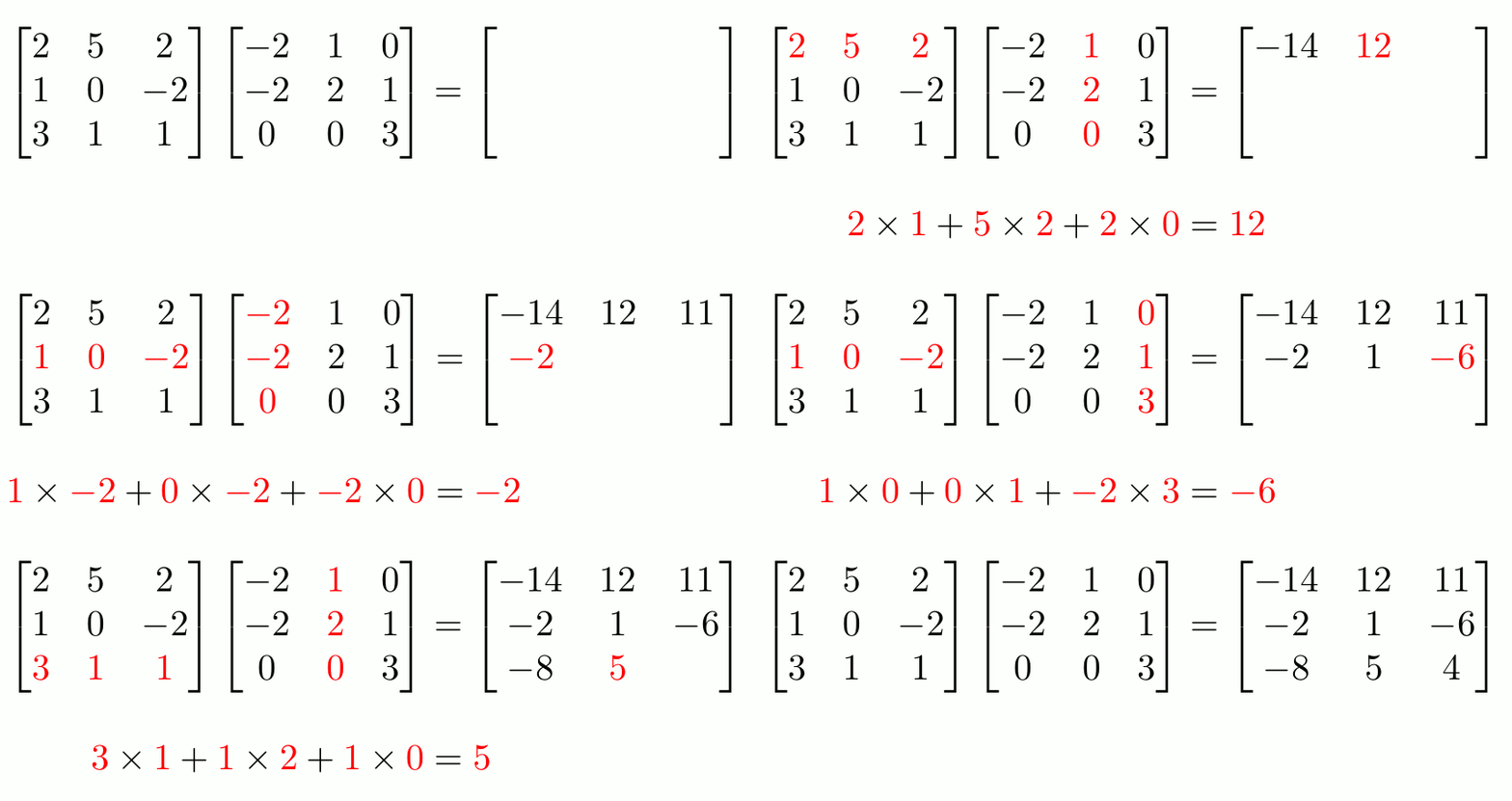
To do actual matrix multiplication<sup>1</sup> (not element-wise), use `%*%`.

:::: {.columns}

::: {.column width="50%"}
```{r}
f_matrix <- c_matrix %*% e_matrix 
f_matrix
```
:::

::: {.column width="50%"}
![1. A reminder of how to do matrix multiplication :)](images/multiply_matrices.gif)
:::

::::

## "Proper" Matrix Math

To invert an invertible square matrix^[![A reminder of how to invert a 2x2 square matrix.](images/inverse_matrix.png)], use `solve()`.

. . . 

```{r}
g_matrix <- solve(f_matrix)
g_matrix
```



## Matrices vs. Data.frames and Tibbles

All of these structures display data in two dimensions

. . . 

:::: {.columns}

::: {.column width="33%"}
+ `matrix`

    + Base `R`
    + Single data type allowed
:::

::: {.column width="34%"}
+ `data.frame`

    + Base `R` 
    + Stores multiple data types
    + Default for data storage
:::

::: {.column width="33%"}
+ `tibbles`

    + `tidyverse`
    + Stores multiple data types
    + Displays nicely
:::

::::

. . . 

In practice, `data.frames` and `tibbles` are very similar!

## Creating `data.frame`s or `tibbles`

We can create a `data.frame` or `tibble` by specifying the columns separately, as individual vectors:

. . . 

:::: {.columns}

::: {.column width="50%"}
```{r}
data.frame(Column1 = c(1, 2, 3),
           Column2 = c("A", "B", "C"))
```
:::

::: {.column width="50%"}
```{r}
tibble(Column1 = c(1, 2, 3),
       Column2 = c("A", "B", "C"))
```
:::

::::

. . . 

*Note:* `data.frame`s and `tibbles` allow for **mixed data types!**

. . . 

This distinction leads us to the final data type, of which `data.frame`s and `tibble`s are a particular subset. 

::: aside
`tibble`'s additional advantages are only displaying the first 10 rows and only the columns that will comfortably fit within the parameters of your console space when called (`data.frame` will display all columns and a certain number of rows depending upon your default max setting - usually this is an overwhelming amount of output, aesthetically confusing,  and not very helpful).
:::

# Lists{.section-title background-color="#99a486"}

## What are Lists?

. . . 

**Lists** are objects that can store multiple types of data.

. . . 

```{r}
my_list <- list(first_thing = 1:5,
                second_thing = matrix(8:11, nrow = 2), 
                third_thing = fct(c("apple", "pear", "banana", "apple", "apple")))
my_list
```

## Accessing List Elements

You can access a list element by its name or number in `[[ ]]`, or a `$` followed by its name:

. . . 

```{r}
my_list[["first_thing"]]
my_list[[1]]
my_list$first_thing
```

## Why Two Brackets `[[` `]]`?

Double brackets get *the actual element* — as whatever data type it is stored as, in that location in the list.

. . . 

```{r}
str(my_list[[1]])
```

. . . 

If you use single brackets to access list elements, you get a **list** back. 

```{r}
str(my_list[1])
```

## `names()` and List Elements

You can use `names()` to get a vector of list element names:

. . . 

```{r}
names(my_list)
```

## `pluck()`

An alternative to using Base `R`'s `[[ ]]` is using `pluck()` from the tidyverse's `purrr` package. 

. . . 

:::: {.columns}

::: {.column width="50%"}
```{r}
obj1 <- list("a", list(1, elt = "foo"))
obj2 <- list("b", list(2, elt = "bar"))
x <- list(obj1, obj2)
x
```
:::

::: {.column width="50%"}
::: {.fragment}
```{r}
pluck(x, 1) 
```

<br>

This is the same as same as `x[[1]]`.

:::
:::

::::

## `pluck()`

An alternative to using Base `R`'s `[[ ]]` is using `pluck()` from the tidyverse's `purrr` package. 

:::: {.columns}

::: {.column width="50%"}
```{r}
obj1 <- list("a", list(1, elt = "foo"))
obj2 <- list("b", list(2, elt = "bar"))
x <- list(obj1, obj2)
x
```
:::

::: {.column width="50%"}
```{r}
pluck(x, 1, 2) 
```

<br>

This is the same as `x[[1]][[2]]`.
:::

::::

## `pluck()`

An alternative to using Base `R`'s `[[ ]]` is using `pluck()` from the tidyverse's `purrr` package. 

:::: {.columns}

::: {.column width="50%"}
```{r}
obj1 <- list("a", list(1, elt = "foo"))
obj2 <- list("b", list(2, elt = "bar"))
x <- list(obj1, obj2)
x
```
:::

::: {.column width="50%"}
```{r}
pluck(x, 1, 2, "elt") 
```

<br>

You can supply names to index into named vectors as well. This is the same as calling `x[[1]][[2]][["elt"]]`. 

:::

::::

## Example: Regression Output <span style="color:#99a486">{{< fa scroll >}}</span> {.scrollable} 

When you perform linear regression in `R`, the output is a list!

. . . 

```{r}
lm_output <- lm(speed ~ dist, data = cars)
is.list(lm_output)
names(lm_output)
lm_output$coefficients
```

. . . 

What does a list object look like?

```{r}
#| output-location: fragment
str(lm_output)
```

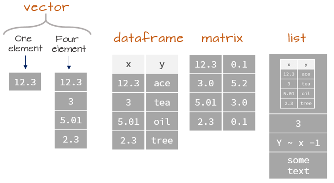
## Data Structures in `R` Overview

. . . 

![](images/data_types_r2.png){fig-align="center" width=200%}

## Data Structures in `R` Overview

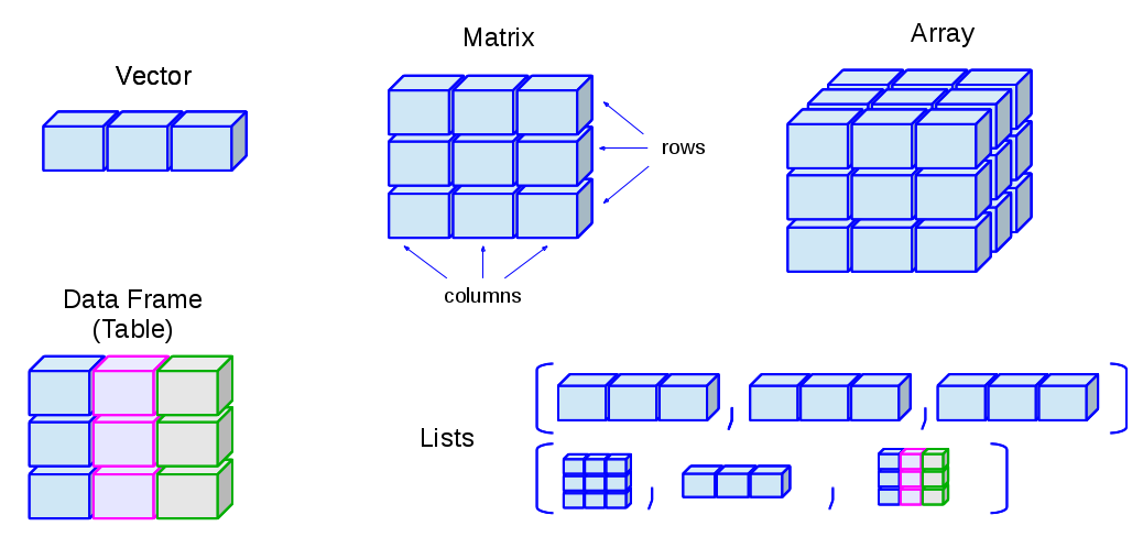![](images/data_types_r3.png){fig-align="center"}

# Lab{.section-title background-color="#99a486"}

## Mini-Check 1: Types of Data & Arithmetic {visibility="hidden"}

In each case, what will R return?

::: {.incremental}
* `is.numeric(pi)`
  + `TRUE`
* `is.integer(3.14)`
  + `FALSE`
* `is.logical(FALSE)`
  + `TRUE`
* `is.nan(NA)`
  + `FALSE`
* `10 %/% 4`
  * `2`
* `10 %% 4`
  * `2`
:::

## Mini-Check 2: Vectors {visibility="hidden"}

::: {.incremental}
* What does `sum(c(1, 2, NA))` output?
  + `NA`. The code `sum(c(1, 2, NA), na.rm = TRUE)` would output `3`.
:::

<br>

::: {.incremental}
* What does `rep(c(0, 1), times = 2)` output?
  + `c(0, 1, 0, 1)`
:::

<br>

::: {.incremental}
* I want to get the first and second elements of my vector, `a_vector`. What's wrong with the code `a_vector[1, 2]` ?
  + `a_vector[c(1, 2)]`
:::

## Matrices and Lists 

1. Write code to create the following matrix:

```{r}
#| echo: false
matrix(c("A", "B", "C", "D", "E", "F"), nrow = 2, byrow = TRUE)
```

2. Write a line of code to extract the second column. Ensure the output is still a *matrix*.

```{r}
#| echo: false
matrix(c("A", "B", "C", "D", "E", "F"), nrow = 2, byrow = TRUE)[ ,2, drop = FALSE]
```

3. Complete the following sentence: "Lists are to vectors, what data frames are to..."

4. Create a list that contains 3 elements: 
    i) `ten_numbers` (integers between 1 and 10)
    ii) `my_name` (your name as a character) 
    iii) `booleans` (vector of `TRUE` and `FALSE` alternating three times)

## Answers

1\. Write code to create the following matrix:

```{r}
matrix_test <- matrix(c("A", "B", "C", "D", "E", "F"), nrow = 2, byrow = TRUE)
matrix_test
```

. . . 

2\. Write a line of code to extract the second column. Ensure the output is still a *matrix*.

```{r}
matrix_test[ ,2, drop = FALSE]
```

## Answers

3\. Complete the following sentence: "Lists are to vectors, what data frames are to...**Matrices!**^[*Lists and data frames can contain mixed data types, while vectors and matrices can only contain one data type. Additionally, lists and vectors are **technically** one dimension while matrices and dataframes are two dimensions.*]" 

. . . 

4\. Create a list that contains 3 elements:

```{r}
my_new_list <- list(ten_numbers = 1:10,
                    my_name = "Victoria Sass",
                    booleans = rep(c(TRUE, FALSE), times = 3))
my_new_list
```

# Homework{.section-title background-color="#1e4655"}

## {data-menu-title="Homework 6" background-iframe="https://vsass.github.io/CSSS508/Homework/HW6/homework6.html" background-interactive=TRUE}