 \n",
"\n",
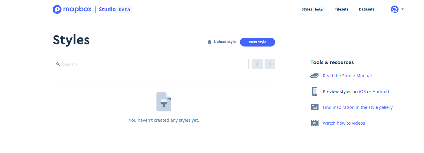
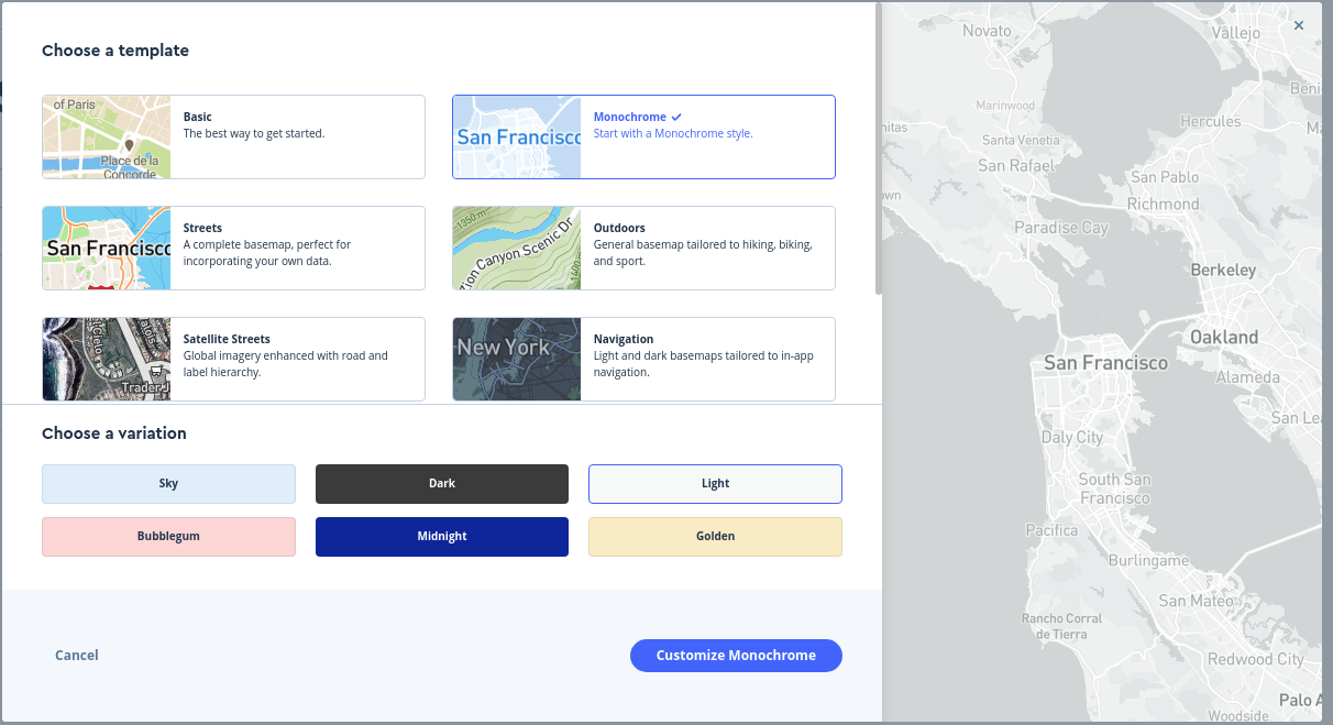
"View the different templates available to you. Given that we are plotting data over a basemap layer, I'd recommend using a template with more muted colors; I have a preference for the \"Monochrome - Light\" version given the way we'll be visualizing our data but I'll let you choose the template you like best. Once you've selected a basemap template, click the \"Customize\" button to advance to the Mapbox Studio editor. \n",
"\n",
"
\n",
"\n",
"View the different templates available to you. Given that we are plotting data over a basemap layer, I'd recommend using a template with more muted colors; I have a preference for the \"Monochrome - Light\" version given the way we'll be visualizing our data but I'll let you choose the template you like best. Once you've selected a basemap template, click the \"Customize\" button to advance to the Mapbox Studio editor. \n",
"\n",
" \n",
"\n",
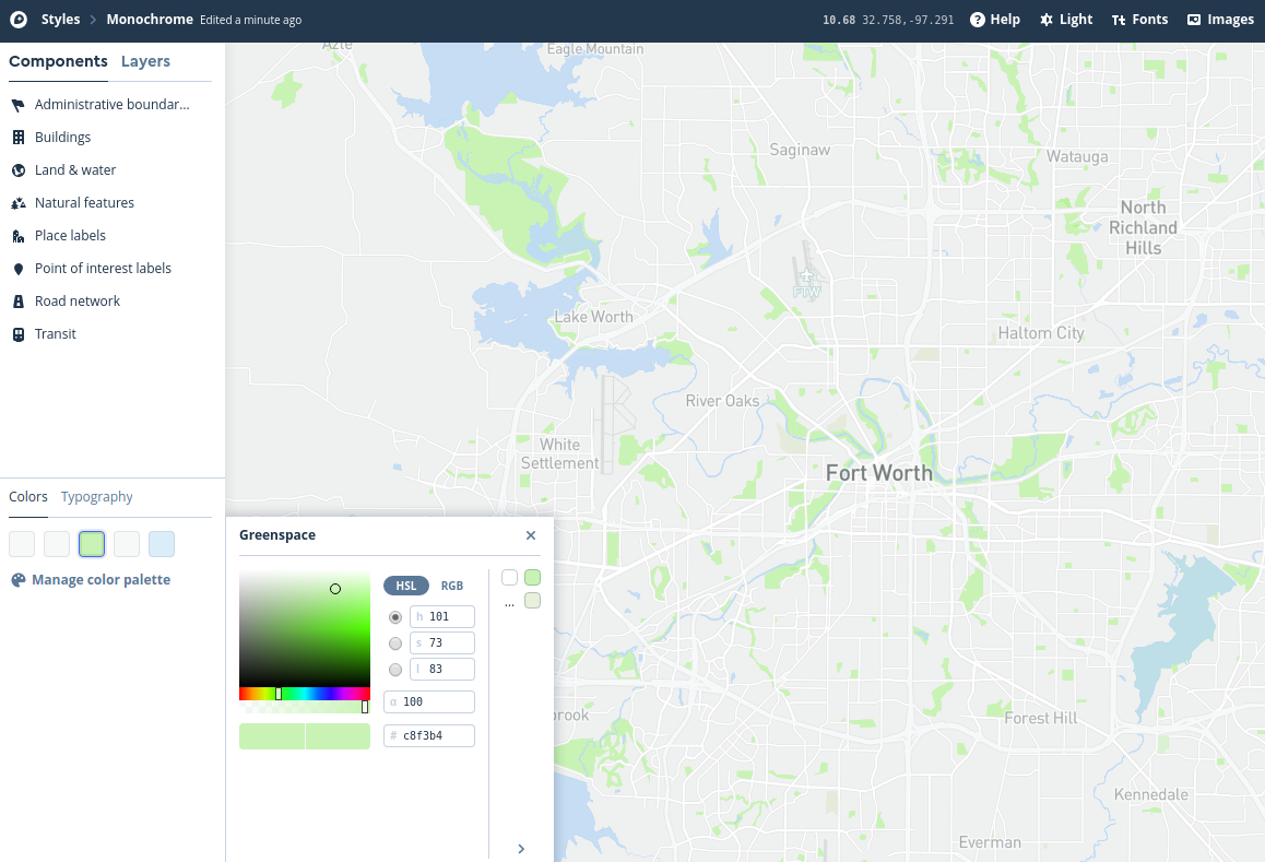
"In the map editor, pan over to the Fort Worth area and zoom in and out. Mapbox Studio gives you access to _vector tiles_, which are variants of the tiled mapping structure we've discussed in class but which expose the underlying data rather than simply showing images. This allows for the customization of any component of the map. You'll see a series of such \"components\" on the left-hand side of the screen. They are organized into categories which you can explore and edit collectively. Alternatively, you can view major categories and style them by clicking the \"Colors\" option in the lower left section of the screen and choosing a map element, then selecting a color from the interactive picker. You can also click the \"Layers\" tab to view all of the individual map layers, and edit them one-by-one; you may need to \"override\" the color to do so. Below, I show an example of the \"Monochrome - Light\" template where I've styled water features with a light blue and park features with a light green. Experiment and try designing a map yourself!\n",
"\n",
""
]
},
{
"cell_type": "markdown",
"metadata": {
"collapsed": false
},
"source": [
"## Loading new data into Mapbox Studio\n",
"\n",
"Now that you've spent some time exploring Mapbox Studio and customizing your map, let's add the public drunkenness data to the map as well to visualize it. Follow these steps to upload your data and add it to the map: \n",
"\n",
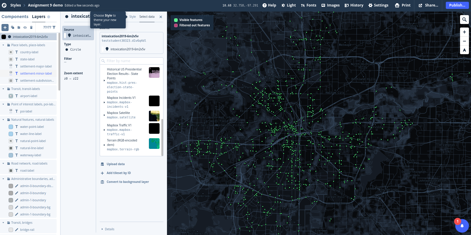
"1. Click \"Layers\" on the left-hand side of the screen and look for the plus sign icon. This will bring up the \"New layer\" menu. \n",
"2. Look for the \"Upload data\" option and click there. Locate your intoxication CSV file and drag and drop it on the dialog box, or click on \"Select a file\" and navigate to it on your computer. You'll see the \"New tileset\" dialog appear; click __Confirm__ if the information is correct.\n",
"3. You'll see a \"Notifications\" box appear in the lower left corner of the screen, letting you know that your upload is processing. Mapbox Studio is converting your public intoxication dataset into vector tiles, which is the same format that is used by the rest of the layers that you've been working with. This will allow you to display your data along with those other layers on the map.\n",
"4. Once your upload has finished processing, scroll down the list of \"Sources\" to the bottom. You should see your intoxication tile source appear as an option. Click there to reveal the point layer within the tileset, then click the revealed layer to add it to your map. You should see your points added to your map. \n",
"\n",
"
\n",
"\n",
"In the map editor, pan over to the Fort Worth area and zoom in and out. Mapbox Studio gives you access to _vector tiles_, which are variants of the tiled mapping structure we've discussed in class but which expose the underlying data rather than simply showing images. This allows for the customization of any component of the map. You'll see a series of such \"components\" on the left-hand side of the screen. They are organized into categories which you can explore and edit collectively. Alternatively, you can view major categories and style them by clicking the \"Colors\" option in the lower left section of the screen and choosing a map element, then selecting a color from the interactive picker. You can also click the \"Layers\" tab to view all of the individual map layers, and edit them one-by-one; you may need to \"override\" the color to do so. Below, I show an example of the \"Monochrome - Light\" template where I've styled water features with a light blue and park features with a light green. Experiment and try designing a map yourself!\n",
"\n",
""
]
},
{
"cell_type": "markdown",
"metadata": {
"collapsed": false
},
"source": [
"## Loading new data into Mapbox Studio\n",
"\n",
"Now that you've spent some time exploring Mapbox Studio and customizing your map, let's add the public drunkenness data to the map as well to visualize it. Follow these steps to upload your data and add it to the map: \n",
"\n",
"1. Click \"Layers\" on the left-hand side of the screen and look for the plus sign icon. This will bring up the \"New layer\" menu. \n",
"2. Look for the \"Upload data\" option and click there. Locate your intoxication CSV file and drag and drop it on the dialog box, or click on \"Select a file\" and navigate to it on your computer. You'll see the \"New tileset\" dialog appear; click __Confirm__ if the information is correct.\n",
"3. You'll see a \"Notifications\" box appear in the lower left corner of the screen, letting you know that your upload is processing. Mapbox Studio is converting your public intoxication dataset into vector tiles, which is the same format that is used by the rest of the layers that you've been working with. This will allow you to display your data along with those other layers on the map.\n",
"4. Once your upload has finished processing, scroll down the list of \"Sources\" to the bottom. You should see your intoxication tile source appear as an option. Click there to reveal the point layer within the tileset, then click the revealed layer to add it to your map. You should see your points added to your map. \n",
"\n",
" \n",
"\n",
"
\n",
"\n",
" \n",
"\n",
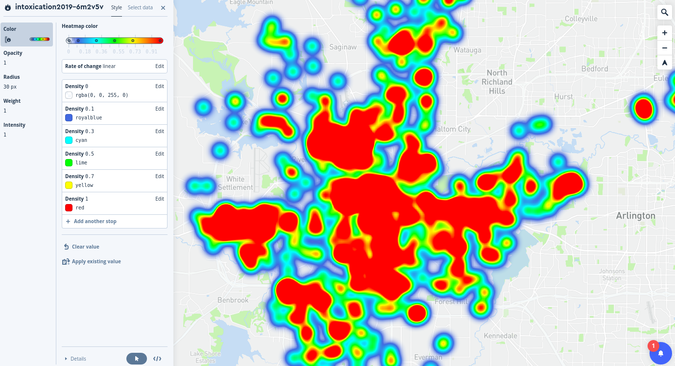
"The visualization defaults to a blue-to-red representation based on five colors, which each represent different density values. The highest density value is scaled to 1, which is bright red; the lowest color value is 0.1 by default, colored blue. Areas without violations are represented without color. Try zooming in and out on your map to see how the heatmap changes based on zoom level. \n",
"\n",
"There are several ways we can make the map more legible, however; I'll outline a few here. \n",
"\n",
"1. When zoomed out to show the entire city, the high-density areas cover most of the urban core. This limits our ability to show differentiation on the map. To modify this, change the __Radius__ of your heatmap from the default 30 pixels and make it smaller. Experiment with different radii and observe how the data representation changes on your map.\n",
"\n",
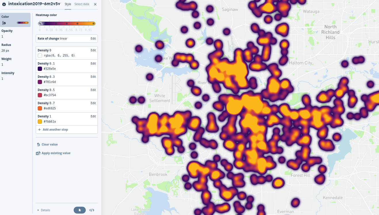
"2. The default color representation, while mapping to perceptions of \"hot\" and \"cold\" is not colorblindness-safe. Make some changes to the color values to use a colorblind-safe palette. I recommend the __viridis__ family of color palettes, which are built into __seaborn__ for quick lookup. There are five palettes in the viridis family: `viridis`, `magma`, `inferno`, `plasma`, and `cividis`. All are color-blind safe, perceptually uniform, and safe to print in black and white. Let's load in the palettes and take a look at them:\n"
]
},
{
"cell_type": "code",
"execution_count": 1,
"metadata": {
"collapsed": false
},
"outputs": [],
"source": [
"import seaborn as sns\n",
"\n",
"viridis = sns.color_palette(\"viridis\", 5).as_hex()\n",
"inferno = sns.color_palette(\"inferno\", 5).as_hex()\n",
"magma = sns.color_palette(\"magma\", 5).as_hex()\n",
"plasma = sns.color_palette(\"plasma\", 5).as_hex()\n",
"cividis = sns.color_palette(\"cividis\", 5).as_hex()"
]
},
{
"cell_type": "markdown",
"metadata": {
"collapsed": false
},
"source": [
"I've assigned five-color extracts from the palettes and converted them to hexadecimal representation, which is a common way to represent colors and can be used in Mapbox Studio. Let's take a look at each palette in turn:"
]
},
{
"cell_type": "code",
"execution_count": 6,
"metadata": {
"collapsed": false
},
"outputs": [
{
"name": "stdout",
"output_type": "stream",
"text": [
"['#443983', '#31688e', '#21918c', '#35b779', '#90d743']\n"
]
},
{
"data": {
"image/png": "iVBORw0KGgoAAAANSUhEUgAAAlEAAACQCAYAAAAoVz7mAAAAOXRFWHRTb2Z0d2FyZQBNYXRwbG90bGliIHZlcnNpb24zLjMuMiwgaHR0cHM6Ly9tYXRwbG90bGliLm9yZy8vihELAAAACXBIWXMAABYlAAAWJQFJUiTwAAADvElEQVR4nO3csYpcZRiA4f+Mm7DDQorR7TeNaKOFhRdi6RV4L15ZwEIIYhW3sEmxIpGFSLL5bbyBfT0zxyHP00z1f3zwM4eXMzDLnHMAAPA4u60XAAA4RyIKACAQUQAAgYgCAAhEFABAIKIAAAIRBQAQiCgAgEBEAQAEIgoAIBBRAACBiAIACC7WHrgsy29jjGdjjNu1ZwMArOxmjPFmzvn8sQdXj6gxxrPd7snhan99OMJsTuD93gvKc/VwObdegf/g4vJh6xWIDk/vt16B6PWr+/Hu7Yd09hgRdXu1vz58+9UPRxjNKdx9fbX1CkR/ftkeBPw/fPb53dYrEH1/82LrFYh+/O7F+P2Xv27LWa8cAAACEQUAEIgoAIBARAEABCIKACAQUQAAgYgCAAhEFABAIKIAAAIRBQAQiCgAgEBEAQAEIgoAIBBRAACBiAIACEQUAEAgogAAAhEFABCIKACAQEQBAAQiCgAgEFEAAIGIAgAIRBQAQCCiAAACEQUAEIgoAIBARAEABCIKACAQUQAAgYgCAAhEFABAIKIAAAIRBQAQiCgAgEBEAQAEIgoAIBBRAACBiAIACEQUAEAgogAAAhEFABCIKACAQEQBAAQiCgAgEFEAAIGIAgAIRBQAQCCiAAACEQUAEIgoAIBARAEABCIKACAQUQAAgYgCAAhEFABAIKIAAAIRBQAQiCgAgEBEAQAEIgoAIBBRAACBiAIACEQUAEAgogAAAhEFABCIKACAQEQBAAQiCgAgEFEAAIGIAgAIRBQAQCCiAAACEQUAEIgoAIBARAEABCIKACAQUQAAgYgCAAhEFABAIKIAAAIRBQAQiCgAgEBEAQAEIgoAIBBRAACBiAIACEQUAEAgogAAAhEFABCIKACAQEQBAAQiCgAgEFEAAIGIAgAIRBQAQCCiAAACEQUAEIgoAIBARAEABCIKACAQUQAAgYgCAAhEFABAIKIAAAIRBQAQLHPOdQcuy91u9+Rwtb9edS6n836vrc/Vw+W632dO6+LyYesViA5P77degej1q/vx7u2HP+acnz727DEi6u8xxidjjJ9XHcypfPHv56+bbkHl/s6Xuztv7u983Ywx3sw5nz/24MX6u4yXY4wx5/zmCLM5smVZfhrD/Z0r93e+3N15c38fJ7/bAAAEIgoAIBBRAACBiAIACEQUAECw+l8cAAB8DLyJAgAIRBQAQCCiAAACEQUAEIgoAIBARAEABCIKACAQUQAAgYgCAAhEFABAIKIAAAIRBQAQiCgAgOAfCtlZGKiX8AUAAAAASUVORK5CYII=",
"text/plain": [
"
\n",
"\n",
"The visualization defaults to a blue-to-red representation based on five colors, which each represent different density values. The highest density value is scaled to 1, which is bright red; the lowest color value is 0.1 by default, colored blue. Areas without violations are represented without color. Try zooming in and out on your map to see how the heatmap changes based on zoom level. \n",
"\n",
"There are several ways we can make the map more legible, however; I'll outline a few here. \n",
"\n",
"1. When zoomed out to show the entire city, the high-density areas cover most of the urban core. This limits our ability to show differentiation on the map. To modify this, change the __Radius__ of your heatmap from the default 30 pixels and make it smaller. Experiment with different radii and observe how the data representation changes on your map.\n",
"\n",
"2. The default color representation, while mapping to perceptions of \"hot\" and \"cold\" is not colorblindness-safe. Make some changes to the color values to use a colorblind-safe palette. I recommend the __viridis__ family of color palettes, which are built into __seaborn__ for quick lookup. There are five palettes in the viridis family: `viridis`, `magma`, `inferno`, `plasma`, and `cividis`. All are color-blind safe, perceptually uniform, and safe to print in black and white. Let's load in the palettes and take a look at them:\n"
]
},
{
"cell_type": "code",
"execution_count": 1,
"metadata": {
"collapsed": false
},
"outputs": [],
"source": [
"import seaborn as sns\n",
"\n",
"viridis = sns.color_palette(\"viridis\", 5).as_hex()\n",
"inferno = sns.color_palette(\"inferno\", 5).as_hex()\n",
"magma = sns.color_palette(\"magma\", 5).as_hex()\n",
"plasma = sns.color_palette(\"plasma\", 5).as_hex()\n",
"cividis = sns.color_palette(\"cividis\", 5).as_hex()"
]
},
{
"cell_type": "markdown",
"metadata": {
"collapsed": false
},
"source": [
"I've assigned five-color extracts from the palettes and converted them to hexadecimal representation, which is a common way to represent colors and can be used in Mapbox Studio. Let's take a look at each palette in turn:"
]
},
{
"cell_type": "code",
"execution_count": 6,
"metadata": {
"collapsed": false
},
"outputs": [
{
"name": "stdout",
"output_type": "stream",
"text": [
"['#443983', '#31688e', '#21918c', '#35b779', '#90d743']\n"
]
},
{
"data": {
"image/png": "iVBORw0KGgoAAAANSUhEUgAAAlEAAACQCAYAAAAoVz7mAAAAOXRFWHRTb2Z0d2FyZQBNYXRwbG90bGliIHZlcnNpb24zLjMuMiwgaHR0cHM6Ly9tYXRwbG90bGliLm9yZy8vihELAAAACXBIWXMAABYlAAAWJQFJUiTwAAADvElEQVR4nO3csYpcZRiA4f+Mm7DDQorR7TeNaKOFhRdi6RV4L15ZwEIIYhW3sEmxIpGFSLL5bbyBfT0zxyHP00z1f3zwM4eXMzDLnHMAAPA4u60XAAA4RyIKACAQUQAAgYgCAAhEFABAIKIAAAIRBQAQiCgAgEBEAQAEIgoAIBBRAACBiAIACC7WHrgsy29jjGdjjNu1ZwMArOxmjPFmzvn8sQdXj6gxxrPd7snhan99OMJsTuD93gvKc/VwObdegf/g4vJh6xWIDk/vt16B6PWr+/Hu7Yd09hgRdXu1vz58+9UPRxjNKdx9fbX1CkR/ftkeBPw/fPb53dYrEH1/82LrFYh+/O7F+P2Xv27LWa8cAAACEQUAEIgoAIBARAEABCIKACAQUQAAgYgCAAhEFABAIKIAAAIRBQAQiCgAgEBEAQAEIgoAIBBRAACBiAIACEQUAEAgogAAAhEFABCIKACAQEQBAAQiCgAgEFEAAIGIAgAIRBQAQCCiAAACEQUAEIgoAIBARAEABCIKACAQUQAAgYgCAAhEFABAIKIAAAIRBQAQiCgAgEBEAQAEIgoAIBBRAACBiAIACEQUAEAgogAAAhEFABCIKACAQEQBAAQiCgAgEFEAAIGIAgAIRBQAQCCiAAACEQUAEIgoAIBARAEABCIKACAQUQAAgYgCAAhEFABAIKIAAAIRBQAQiCgAgEBEAQAEIgoAIBBRAACBiAIACEQUAEAgogAAAhEFABCIKACAQEQBAAQiCgAgEFEAAIGIAgAIRBQAQCCiAAACEQUAEIgoAIBARAEABCIKACAQUQAAgYgCAAhEFABAIKIAAAIRBQAQiCgAgEBEAQAEIgoAIBBRAACBiAIACEQUAEAgogAAAhEFABCIKACAQEQBAAQiCgAgEFEAAIGIAgAIRBQAQCCiAAACEQUAEIgoAIBARAEABCIKACAQUQAAgYgCAAhEFABAIKIAAAIRBQAQLHPOdQcuy91u9+Rwtb9edS6n836vrc/Vw+W632dO6+LyYesViA5P77degej1q/vx7u2HP+acnz727DEi6u8xxidjjJ9XHcypfPHv56+bbkHl/s6Xuztv7u983Ywx3sw5nz/24MX6u4yXY4wx5/zmCLM5smVZfhrD/Z0r93e+3N15c38fJ7/bAAAEIgoAIBBRAACBiAIACEQUAECw+l8cAAB8DLyJAgAIRBQAQCCiAAACEQUAEIgoAIBARAEABCIKACAQUQAAgYgCAAhEFABAIKIAAAIRBQAQiCgAgOAfCtlZGKiX8AUAAAAASUVORK5CYII=",
"text/plain": [
" \n",
"\n",
"If you'd like, you can also modify the \"stops\" that correspond to each color value to tune the color blending accordingly.\n",
"\n"
]
},
{
"cell_type": "markdown",
"metadata": {
"collapsed": false
},
"source": [
"3. While the color scheme is now more appropriate, it is difficult to understand _where_ the concentrations of violations are because your heatmap is fully opaque. Choose the __Opacity__ option and lower the value to make your heatmap layer semi-transparent. You might also consider modifying the __Weight__ and __Intensity__ options to make your heatmap less intense. Experiment with these different options until you achieve a representation that you like. \n",
"\n",
"4. Finally, integrate your heatmap's relationship better with the other map layers by modifying its positioning. You may notice on the left-hand side of the screen that each element of the map - from map labels to roadways to water features - is represented in hierarchical order, with your heatmap layer sitting at the very top. Click your intoxication layer in the layer list and drag it beneath all of the label layers (the last one listed is \"road-label\") and note how the visual hierarchy of your map changes, with labels above your heatmap."
]
},
{
"cell_type": "markdown",
"metadata": {
"collapsed": false
},
"source": [
"## Sharing your map\n",
"\n",
"Now that you've made modifications to your map visualization, it is ready to share! Click the __Publish__ button in the top right corner of your screen to publish your map. Once published, click __Continue editing__. There are a couple different ways that you can share your map. The __Print__ button allows you to export your map as a static image. The __Share__ button gives you a series of options for sharing your map either as a standalone interactive map or as an embedded element in a mobile or web application. Click __Share__, and note the URL which you can copy in the __Share style__ section. Click the \"Make Public\" button to make your style share-able, then try copying this URL and pasting in a web browser; you'll see your map appear full-screen. \n",
"\n",
"Below this section, note the __Developer resources__. This gives you some resources to embed your map in a website or a mobile application. To complete this assignment, you'll get some small experience embedding the Mapbox map that you've designed in a stand-alone web page using Mapbox GL, Mapbox's web development library.\n",
"\n",
"If you haven't already, download the HTML file from TCU Online named \"example_map.html\". Open the HTML file in a text editor, not a web browser. To do this, either right-click the downloaded file and choose an option to open the file in a text editor (e.g. Notepad on Windows or TextEdit on a Mac), or open the text editor first, choose __Open__, and navigate to your HTML file. \n",
"\n",
"You'll see some HTML code that I've copied from [the Mapbox \"Display a map\" tutorial](https://docs.mapbox.com/mapbox-gl-js/example/simple-map/). You don't need to understand everything that is going on here, but I do want to get you some practice modifying it. The HTML file is a text file that can be interpreted by web browsers and rendered as a website. It can be downloaded and hosted on your personal website, for example. \n",
"\n",
"Look for the section inside the `` tags that appears as below:\n",
"\n",
"```html\n",
"\n",
"\n",
"```\n",
"\n",
"Copy the \"Access token\" from your Share dialog in Mapbox Studio (it starts with \"pk.\") and replace the existing access token in the HTML code with your own. Next, do the same for the style URL. Save the map file, then try opening it in a web browser (navigate to the file through your computer's filesystem, then double-click the file to launch it). If it does not appear immediately, it is because the styles take a few moments to publish after you've first published them; you can add the text `/draft` directly after your style URL to view it right away (I have this example saved for illustration).\n",
"\n",
"## For submission\n",
"\n",
"To get credit for this assignment, modify the `example_map.html` file as instructed above with your Mapbox access token and style URL and upload your map file to the submission console in TCU Online. This will allow me to view your map!"
]
},
{
"cell_type": "code",
"execution_count": null,
"metadata": {
"collapsed": false
},
"outputs": [],
"source": []
}
],
"metadata": {
"interpreter": {
"hash": "2b9421c38bd9785733c8ab589f124ba12ef5207025179e9d09f8a045acc4fc72"
},
"kernelspec": {
"display_name": "Python 3.9.5 64-bit ('python39': conda)",
"name": "python3"
},
"language_info": {
"codemirror_mode": {
"name": "ipython",
"version": 3
},
"file_extension": ".py",
"mimetype": "text/x-python",
"name": "python",
"nbconvert_exporter": "python",
"pygments_lexer": "ipython3",
"version": "3.11.6"
}
},
"nbformat": 4,
"nbformat_minor": 4
}
\n",
"\n",
"If you'd like, you can also modify the \"stops\" that correspond to each color value to tune the color blending accordingly.\n",
"\n"
]
},
{
"cell_type": "markdown",
"metadata": {
"collapsed": false
},
"source": [
"3. While the color scheme is now more appropriate, it is difficult to understand _where_ the concentrations of violations are because your heatmap is fully opaque. Choose the __Opacity__ option and lower the value to make your heatmap layer semi-transparent. You might also consider modifying the __Weight__ and __Intensity__ options to make your heatmap less intense. Experiment with these different options until you achieve a representation that you like. \n",
"\n",
"4. Finally, integrate your heatmap's relationship better with the other map layers by modifying its positioning. You may notice on the left-hand side of the screen that each element of the map - from map labels to roadways to water features - is represented in hierarchical order, with your heatmap layer sitting at the very top. Click your intoxication layer in the layer list and drag it beneath all of the label layers (the last one listed is \"road-label\") and note how the visual hierarchy of your map changes, with labels above your heatmap."
]
},
{
"cell_type": "markdown",
"metadata": {
"collapsed": false
},
"source": [
"## Sharing your map\n",
"\n",
"Now that you've made modifications to your map visualization, it is ready to share! Click the __Publish__ button in the top right corner of your screen to publish your map. Once published, click __Continue editing__. There are a couple different ways that you can share your map. The __Print__ button allows you to export your map as a static image. The __Share__ button gives you a series of options for sharing your map either as a standalone interactive map or as an embedded element in a mobile or web application. Click __Share__, and note the URL which you can copy in the __Share style__ section. Click the \"Make Public\" button to make your style share-able, then try copying this URL and pasting in a web browser; you'll see your map appear full-screen. \n",
"\n",
"Below this section, note the __Developer resources__. This gives you some resources to embed your map in a website or a mobile application. To complete this assignment, you'll get some small experience embedding the Mapbox map that you've designed in a stand-alone web page using Mapbox GL, Mapbox's web development library.\n",
"\n",
"If you haven't already, download the HTML file from TCU Online named \"example_map.html\". Open the HTML file in a text editor, not a web browser. To do this, either right-click the downloaded file and choose an option to open the file in a text editor (e.g. Notepad on Windows or TextEdit on a Mac), or open the text editor first, choose __Open__, and navigate to your HTML file. \n",
"\n",
"You'll see some HTML code that I've copied from [the Mapbox \"Display a map\" tutorial](https://docs.mapbox.com/mapbox-gl-js/example/simple-map/). You don't need to understand everything that is going on here, but I do want to get you some practice modifying it. The HTML file is a text file that can be interpreted by web browsers and rendered as a website. It can be downloaded and hosted on your personal website, for example. \n",
"\n",
"Look for the section inside the `` tags that appears as below:\n",
"\n",
"```html\n",
"\n",
"\n",
"```\n",
"\n",
"Copy the \"Access token\" from your Share dialog in Mapbox Studio (it starts with \"pk.\") and replace the existing access token in the HTML code with your own. Next, do the same for the style URL. Save the map file, then try opening it in a web browser (navigate to the file through your computer's filesystem, then double-click the file to launch it). If it does not appear immediately, it is because the styles take a few moments to publish after you've first published them; you can add the text `/draft` directly after your style URL to view it right away (I have this example saved for illustration).\n",
"\n",
"## For submission\n",
"\n",
"To get credit for this assignment, modify the `example_map.html` file as instructed above with your Mapbox access token and style URL and upload your map file to the submission console in TCU Online. This will allow me to view your map!"
]
},
{
"cell_type": "code",
"execution_count": null,
"metadata": {
"collapsed": false
},
"outputs": [],
"source": []
}
],
"metadata": {
"interpreter": {
"hash": "2b9421c38bd9785733c8ab589f124ba12ef5207025179e9d09f8a045acc4fc72"
},
"kernelspec": {
"display_name": "Python 3.9.5 64-bit ('python39': conda)",
"name": "python3"
},
"language_info": {
"codemirror_mode": {
"name": "ipython",
"version": 3
},
"file_extension": ".py",
"mimetype": "text/x-python",
"name": "python",
"nbconvert_exporter": "python",
"pygments_lexer": "ipython3",
"version": "3.11.6"
}
},
"nbformat": 4,
"nbformat_minor": 4
}