## mapboxapi
[](https://CRAN.R-project.org/package=mapboxapi) 
An R interface to Mapbox APIs and web services
The purpose of {mapboxapi} is to facilitate the use of [Mapbox web services](https://docs.mapbox.com/api/) for spatial data science tasks in R. Current and future versions of the package allow R users to return Mapbox navigation requests as simple features (sf) objects, convert R objects to Mapbox vector tilesets, and query Mapbox tilesets from R, among other tasks. The package is not a complete wrapper of the API (though new features will continually be added) nor is it an interface to [Mapbox GL JS](https://docs.mapbox.com/mapbox-gl-js/api/), Mapbox's web mapping API.
Install the package from CRAN then store your Mapbox access token for use in the package:
```r
install.packages("mapboxapi")
# For the development version:
# remotes::install_github("walkerke/mapboxapi")
# Get your access token from your Mapbox account and save it in R; save a public token,
# secret token, or both with successive calls to mb_access_token()
mapboxapi::mb_access_token("pk.eyzdl....", install = TRUE)
```
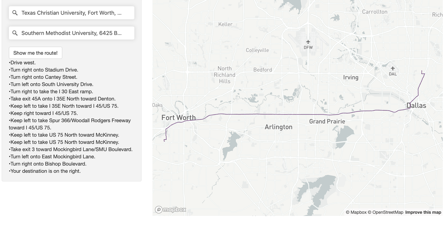
#### Example 1: Building a routing app with Shiny and `mb_directions()`
```r
library(shiny)
library(mapdeck)
library(mapboxapi)
# Set up a sidebar panel with geocoders for origin and destination,
# and a placeholder to print out the driving instructions
ui <- fluidPage(
tags$head(
tags$style(HTML(
"#origin {
position: relative;
z-index: 999999;
}"
))
),
sidebarPanel(
mapboxGeocoderInput("origin", placeholder = "Enter an origin",
proximity = mb_geocode("Fort Worth, TX")),
shiny::br(),
mapboxGeocoderInput("destination", placeholder = "Enter a destination",
proximity = mb_geocode("Fort Worth, TX")),
shiny::br(),
actionButton("action", "Show me the route!"),
htmlOutput("instructions"),
width = 4
),
mainPanel(
mapdeckOutput(outputId = "map", width = "100%", height = 600)
)
)
# Set up reactive elements to generate routes when the action button is clicked,
# then map the routes and print out the driving directions
server <- function(input, output) {
output$map <- renderMapdeck({
mapdeck(token = Sys.getenv("MAPBOX_PUBLIC_TOKEN"),
style = mapdeck_style("light"),
zoom = 11,
location = c(-97.3034314, 32.7593745))
})
new_route <- eventReactive(input$action, {
mb_directions(
input_data = rbind(
geocoder_as_sf(input$origin),
geocoder_as_sf(input$destination)
),
profile = "driving",
output = "sf",
steps = TRUE
)
})
observeEvent(new_route(), {
mapdeck_update(map_id = "map") %>%
clear_path(layer_id = "new_route") %>%
add_path(data = new_route(), stroke_width = 75,
layer_id = "new_route", update_view = TRUE,
focus_layer = TRUE)
output$instructions <- renderUI({
HTML(paste0(
paste("•", new_route()$instruction, sep = ""),
collapse = "
"))
})
})
}
shinyApp(ui = ui, server = server)
```
 #### Example 2: render large datasets as scalable vector tiles with tippecanoe
```r
library(mapboxapi)
library(mapdeck)
library(httr)
# Get the Microsoft buildings data for Texas and unzip
GET("https://usbuildingdata.blob.core.windows.net/usbuildings-v1-1/Texas.zip",
write_disk("Texas.zip", overwrite = TRUE), progress())
unzip("Texas.zip")
# Use tippecanoe to make a dynamic .mbtiles file that visualizes large data appropriately
# at any zoom level. sf objects can also be used as input!
# (requires installing tippecanoe on your machine separately first)
tippecanoe(input = "Texas.geojson",
output = "Texas.mbtiles",
layer_name = "texas_buildings")
# Upload the generated tileset to your Mapbox account (requires a Mapbox secret access token
# to be set as an environment variable)
upload_tiles(input = "Texas.mbtiles", username = "kwalkertcu",
tileset_id = "TX_buildings",
multipart = TRUE)
# Head over to Mapbox Studio when the upload is done (check the status with
# `check_upload_status()`) and add it to a style. When you've styled it, bring it back
# into R with mapdeck by referencing the style ID:
mapdeck(token = Sys.getenv("MAPBOX_PUBLIC_TOKEN"),
style = "mapbox://styles/kwalkertcu/ckaf9qxim1pyk1io7r2e8exj2/draft",
zoom = 6,
location = c(-98.7382803, 31.7678448))
```
### Example 3: a research workflow to determine how median gross rent varies by distance from downtown
```r
library(mapboxapi)
library(tidyverse)
library(tidycensus)
library(tigris)
library(sf)
library(crsuggest)
options(tigris_use_cache = TRUE)
# Grab median gross rent data from the ACS for the Twin Cities metro
county_names <- c("Hennepin", "Ramsey", "Anoka", "Washington",
"Dakota", "Carver", "Scott")
tc_rent <- get_acs(geography = "tract",
variables = "B25064_001",
state = "MN",
county = county_names,
year = 2022,
geometry = TRUE)
# Find the right coordinate system to use; in this case we'll use 26993
print(suggest_top_crs(tc_rent, units = "m"))
# Remove water areas - there are a lot in Minnesota! - to help ensure that a point in a
# given Census tract will be routable
tc_rent_points <- tc_rent %>%
st_transform(26993) %>%
erase_water(area_threshold = 0.95) %>%
st_point_on_surface()
# Determine the location of downtown (apologies to St. Paul, purposes of illustration here)
downtown_mpls <- mb_geocode("Minneapolis City Hall, Minneapolis MN")
# Use mb_matrix() to calculate driving time from all Twin Cities Census tracts to downtown
time_to_downtown <- mb_matrix(origins = tc_rent_points,
destinations = downtown_mpls) %>%
as.vector()
tc_rent$time <- time_to_downtown
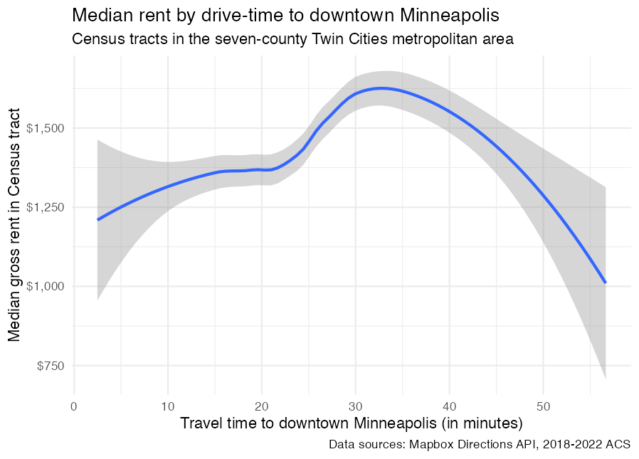
# Visualize how rent varies by travel time from downtown with ggplot2
ggplot(tc_rent, aes(x = time, y = estimate)) +
geom_smooth() +
scale_y_continuous(labels = scales::dollar) +
labs(x = "Travel time to downtown Minneapolis (in minutes)",
y = "Median gross rent in Census tract",
title = "Median rent by drive-time to downtown Minneapolis",
subtitle = "Census tracts in the seven-county Twin Cities metropolitan area",
caption = "Data sources: Mapbox Directions API, 2018-2022 ACS") +
theme_minimal()
```
#### Example 2: render large datasets as scalable vector tiles with tippecanoe
```r
library(mapboxapi)
library(mapdeck)
library(httr)
# Get the Microsoft buildings data for Texas and unzip
GET("https://usbuildingdata.blob.core.windows.net/usbuildings-v1-1/Texas.zip",
write_disk("Texas.zip", overwrite = TRUE), progress())
unzip("Texas.zip")
# Use tippecanoe to make a dynamic .mbtiles file that visualizes large data appropriately
# at any zoom level. sf objects can also be used as input!
# (requires installing tippecanoe on your machine separately first)
tippecanoe(input = "Texas.geojson",
output = "Texas.mbtiles",
layer_name = "texas_buildings")
# Upload the generated tileset to your Mapbox account (requires a Mapbox secret access token
# to be set as an environment variable)
upload_tiles(input = "Texas.mbtiles", username = "kwalkertcu",
tileset_id = "TX_buildings",
multipart = TRUE)
# Head over to Mapbox Studio when the upload is done (check the status with
# `check_upload_status()`) and add it to a style. When you've styled it, bring it back
# into R with mapdeck by referencing the style ID:
mapdeck(token = Sys.getenv("MAPBOX_PUBLIC_TOKEN"),
style = "mapbox://styles/kwalkertcu/ckaf9qxim1pyk1io7r2e8exj2/draft",
zoom = 6,
location = c(-98.7382803, 31.7678448))
```
### Example 3: a research workflow to determine how median gross rent varies by distance from downtown
```r
library(mapboxapi)
library(tidyverse)
library(tidycensus)
library(tigris)
library(sf)
library(crsuggest)
options(tigris_use_cache = TRUE)
# Grab median gross rent data from the ACS for the Twin Cities metro
county_names <- c("Hennepin", "Ramsey", "Anoka", "Washington",
"Dakota", "Carver", "Scott")
tc_rent <- get_acs(geography = "tract",
variables = "B25064_001",
state = "MN",
county = county_names,
year = 2022,
geometry = TRUE)
# Find the right coordinate system to use; in this case we'll use 26993
print(suggest_top_crs(tc_rent, units = "m"))
# Remove water areas - there are a lot in Minnesota! - to help ensure that a point in a
# given Census tract will be routable
tc_rent_points <- tc_rent %>%
st_transform(26993) %>%
erase_water(area_threshold = 0.95) %>%
st_point_on_surface()
# Determine the location of downtown (apologies to St. Paul, purposes of illustration here)
downtown_mpls <- mb_geocode("Minneapolis City Hall, Minneapolis MN")
# Use mb_matrix() to calculate driving time from all Twin Cities Census tracts to downtown
time_to_downtown <- mb_matrix(origins = tc_rent_points,
destinations = downtown_mpls) %>%
as.vector()
tc_rent$time <- time_to_downtown
# Visualize how rent varies by travel time from downtown with ggplot2
ggplot(tc_rent, aes(x = time, y = estimate)) +
geom_smooth() +
scale_y_continuous(labels = scales::dollar) +
labs(x = "Travel time to downtown Minneapolis (in minutes)",
y = "Median gross rent in Census tract",
title = "Median rent by drive-time to downtown Minneapolis",
subtitle = "Census tracts in the seven-county Twin Cities metropolitan area",
caption = "Data sources: Mapbox Directions API, 2018-2022 ACS") +
theme_minimal()
```