Chapter 6: WRF-Var

 

Table of Contents

• Introduction
• Installing WRF-Var
• Installing WRFNL and WRFPLUS
• Running Observation Preprocessor (OBSPROC)
• Running WRF-Var
• Radiance Data Assimilations in WRF-Var
• WRF-Var Diagnostics
• Updating WRF boundary conditions
• Running gen_be
• Additional WRF-Var Exercises
• Description of Namelist Variables

 

Introduction

Data assimilation is the technique by which observations are combined with a NWP product (the first guess or background forecast) and their respective error statistics to provide an improved estimate (the analysis) of the atmospheric (or oceanic, Jovian, whatever) state. Variational (Var) data assimilation achieves this through the iterative minimization of a prescribed cost (or penalty) function. Differences between the analysis and observations/first guess are penalized (damped) according to their perceived error. The difference between three-dimensional (3D-Var) and four-dimensional (4D-Var) data assimilation is the use of a numerical forecast model in the latter.

MMM Division of NCAR supports a unified (global/regional, multi-model, 3/4D-Var) model-space variational data assimilation system (WRF-Var) for use by NCAR staff and collaborators, and is also freely available to the general community, together with further documentation, test results, plans etc., from the WRF-Var web-page http://www.mmm.ucar.edu/wrf/users/wrfda/Docs/user_guide_V3.1.1/users_guide_chap6.htm.

Various components of the WRF-Var system are shown in blue in the sketch below, together with their relationship with rest of the WRF system.

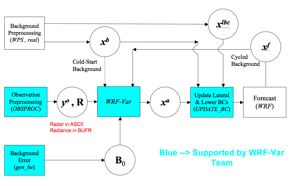
x^b: first guess either from previous WRF forecast or from WPS/real output.

x^lbc: lateral boundary from WPS/real output.

x^a: analysis from WRF-Var data assimilation system.

x^f: WRF forecast output.

y^o: observations processed by OBSPROC. (note: Radar and Radiance data don’t go through OBSPROC)

B₀: background error statistics from generic be.data/gen_be.

R: observational and representativeness data error statistics.

In this chapter, you will learn how to run the various components of WRF-Var system. For the training purpose, you are supplied with a test case including the following input data: a) observation file (in the format prior to OBSPROC), b) WRF NetCDF background file (WPS/real output used as a first guess of the analysis), and c) Background error statistics (estimate of errors in the background file). You can download the test dataset from http://www.mmm.ucar.edu/wrf/users/wrfda/download/testdata.html. In your own work, you have to create all these input files yourselves. See the section Running Observation Preprocessor for creating your observation files. See section Running gen_be for generating your background error statistics file if you want to use cv_options=5.

Before using your own data, we suggest that you start by running through the WRF-Var related programs at least once using the supplied test case. This serves two purposes: First, you can learn how to run the programs with data we have tested ourselves, and second you can test whether your computer is adequate to run the entire modeling system. After you have done the tutorial, you can try running other, more computationally intensive, case studies and experimenting with some of the many namelist variables.

 

WARNING: It is impossible to test every code upgrade with every permutation of computer, compiler, number of processors, case, namelist option, etc. The “namelist” options that are supported are indicated in the “WRFDA/var/README.namelist” and these are the default options.

Running with your own domain. Hopefully, our test cases will have prepared you for the variety of ways in which you may wish to run WRF-Var. Please let us know your experiences.

As a professional courtesy, we request that you include the following reference in any publications that makes use of any component of the community WRF-Var system:

 

Barker, D.M., W. Huang, Y. R. Guo, and Q. N. Xiao., 2004: A Three-Dimensional (3DVAR) Data Assimilation System For Use With MM5: Implementation and Initial Results. Mon. Wea. Rev., 132, 897-914.

 

Huang, X.Y., Q. Xiao, D.M. Barker, X. Zhang, J. Michalakes, W. Huang, T. Henderson, J. Bray, Y. Chen, Z. Ma, J. Dudhia, Y. Guo, X. Zhang, D.J. Won, H.C. Lin, and Y.H. Kuo, 2009: Four-Dimensional Variational Data Assimilation for WRF: Formulation and Preliminary Results. Mon. Wea. Rev., 137, 299–314.

Running WRF-Var requires a Fortran 90 compiler. We currently have currently tested the WRF-Var on the following platforms: IBM (XLF), SGI Altix (INTEL), PC/Linux (PGI, INTEL, GFORTRAN), and Apple (G95/PGI). Please let us know if this does not meet your requirements, and we will attempt to add other machines to our list of supported architectures as resources allow. Although we are interested to hear of your experiences on modifying compile options, we do not yet recommend making changes to the configure file used to compile WRF-Var.

 

Installing WRF-Var

Start with V3.1.1, to compile the WRF-Var code, it is necessary to have installed the NetCDF library if only conventional observational data from LITTLE_R format file is to be used.

If you intend to use observational data with PREPBUFR format, an environment variables is needed to be set like (using the C-shell),

> setenv BUFR 1

If you intend to assimilate satellite radiance data, in addition to BUFR library, either CRTM (V1.2) or RTTOV (8.7) have to be installed and they can be downloaded from ftp://ftp.emc.ncep.noaa.gov/jcsda/CRTM/ and http://www.metoffice.gov.uk/science/creating/working_together/nwpsaf_public.html. The additional necessary environment variables needed are set (again using the C-shell), by commands looking something like

> setenv RTTOV /usr/local/rttov87

(Note: make a linkage of $RTTOV/librttov.a to $RTTOV/src/librttov8.7.a)
> setenv CRTM /usr/local/crtm

(Note: make a linkage of $CRTM/libcrtm.a to $CRTM/src/libCRTM.a )

Note: Make sure the required libraries were all compiled using the same compiler that will be used to build WRF-Var, since the libraries produced by one compiler may not be compatible with code compiled with another.

Assuming all required libraries are available, the WRF-Var source code can be downloaded from http://www.mmm.ucar.edu/wrf/users/wrfda/download/get_source.html. After the tar file is unzipped (gunzip WRFDAV3_1_1.TAR.gz) and untarred (untar WRFDAV3_1_1.TAR), the directory WRFDA should be created; this directory contains the WRF-Var source code.

To configure WRF-Var, change to the WRFDA directory and type

> ./configure wrfda

A list of configuration options for your computer should appear. Each option combines a compiler type and a parallelism option; since the configuration script doesn’t check which compilers are actually available, be sure to only select among the options for compilers that are available on your system. The parallelism option allows for a single-processor (serial) compilation, shared-memory parallel (smpar) compilation, distributed-memory parallel (dmpar) compilation and distributed-memory with shared-memory parallel (sm+dm) compilation. For example, on a Macintosh computer, the above steps look like:

> ./configure wrfda

checking for perl5... no

checking for perl... found /usr/bin/perl (perl)

Will use NETCDF in dir: /users/noname/work/external/g95/netcdf-3.6.1

PHDF5 not set in environment. Will configure WRF for use without.

$JASPERLIB or $JASPERINC not found in environment, configuring to build without grib2 I/O...

------------------------------------------------------------------------

Please select from among the following supported platforms.

 

1. Darwin (MACOS) PGI compiler with pgcc (serial)

2. Darwin (MACOS) PGI compiler with pgcc (smpar)

3. Darwin (MACOS) PGI compiler with pgcc (dmpar)

4. Darwin (MACOS) PGI compiler with pgcc (dm+sm)

5. Darwin (MACOS) intel compiler with icc (serial)

6. Darwin (MACOS) intel compiler with icc (smpar)

7. Darwin (MACOS) intel compiler with icc (dmpar)

8. Darwin (MACOS) intel compiler with icc (dm+sm)

9. Darwin (MACOS) intel compiler with cc (serial)

10. Darwin (MACOS) intel compiler with cc (smpar)

11. Darwin (MACOS) intel compiler with cc (dmpar)

12. Darwin (MACOS) intel compiler with cc (dm+sm)

13. Darwin (MACOS) g95 with gcc (serial)

14. Darwin (MACOS) g95 with gcc (dmpar)

15. Darwin (MACOS) xlf (serial)

16. Darwin (MACOS) xlf (dmpar)

 

Enter selection [1-10] : 13

------------------------------------------------------------------------

Compile for nesting? (0=no nesting, 1=basic, 2=preset moves, 3=vortex following) [default 0]:

Configuration successful. To build the model type compile .

……

After running the configure script and choosing a compilation option, a configure.wrf file will be created. Because of the variety of ways that a computer can be configured, if the WRF-Var build ultimately fails, there is a chance that minor modifications to the configure.wrf file may be needed.

Note: WRF compiles with –r4 option while WRFDA compiles with –r8. For this reason, WRF and WRFDA cannot reside and be compiled under the same directory.

Hint: It is helpful to start with something simple, such as the serial build. If it is successful, move on to build dmpar code. Remember to type ‘clean –a’ between each build.

To compile the code, type

> ./compile all_wrfvar >&! compile.out

Successful compilation of ‘all_wrfvar” will produce 31 executables in the var/build directory which are linked in var/da directory, as well as obsproc.exe in var/obsproc/src directory. You can list these executables by issuing the command (from WRFDA directory)

> ls -l var/build/*exe var/obsproc/src/obsproc.exe

-rwxr-xr-x 1 noname users 641048 Mar 23 09:28 var/build/da_advance_time.exe

-rwxr-xr-x 1 noname users 954016 Mar 23 09:29 var/build/da_bias_airmass.exe

-rwxr-xr-x 1 noname users 721140 Mar 23 09:29 var/build/da_bias_scan.exe

-rwxr-xr-x 1 noname users 686652 Mar 23 09:29 var/build/da_bias_sele.exe

-rwxr-xr-x 1 noname users 700772 Mar 23 09:29 var/build/da_bias_verif.exe

-rwxr-xr-x 1 noname users 895300 Mar 23 09:29 var/build/da_rad_diags.exe

-rwxr-xr-x 1 noname users 742660 Mar 23 09:29 var/build/da_tune_obs_desroziers.exe

-rwxr-xr-x 1 noname users 942948 Mar 23 09:29 var/build/da_tune_obs_hollingsworth1.exe

-rwxr-xr-x 1 noname users 913904 Mar 23 09:29 var/build/da_tune_obs_hollingsworth2.exe

-rwxr-xr-x 1 noname users 943000 Mar 23 09:28 var/build/da_update_bc.exe

-rwxr-xr-x 1 noname users 1125892 Mar 23 09:29 var/build/da_verif_anal.exe

-rwxr-xr-x 1 noname users 705200 Mar 23 09:29 var/build/da_verif_obs.exe

-rwxr-xr-x 1 noname users 46602708 Mar 23 09:28 var/build/da_wrfvar.exe

-rwxr-xr-x 1 noname users 1938628 Mar 23 09:29 var/build/gen_be_cov2d.exe

-rwxr-xr-x 1 noname users 1938628 Mar 23 09:29 var/build/gen_be_cov3d.exe

-rwxr-xr-x 1 noname users 1930436 Mar 23 09:29 var/build/gen_be_diags.exe

-rwxr-xr-x 1 noname users 1942724 Mar 23 09:29 var/build/gen_be_diags_read.exe

-rwxr-xr-x 1 noname users 1941268 Mar 23 09:29 var/build/gen_be_ensmean.exe

-rwxr-xr-x 1 noname users 1955192 Mar 23 09:29 var/build/gen_be_ensrf.exe

-rwxr-xr-x 1 noname users 1979588 Mar 23 09:28 var/build/gen_be_ep1.exe

-rwxr-xr-x 1 noname users 1961948 Mar 23 09:28 var/build/gen_be_ep2.exe

-rwxr-xr-x 1 noname users 1945360 Mar 23 09:29 var/build/gen_be_etkf.exe

-rwxr-xr-x 1 noname users 1990936 Mar 23 09:28 var/build/gen_be_stage0_wrf.exe

-rwxr-xr-x 1 noname users 1955012 Mar 23 09:28 var/build/gen_be_stage1.exe

-rwxr-xr-x 1 noname users 1967296 Mar 23 09:28 var/build/gen_be_stage1_1dvar.exe

-rwxr-xr-x 1 noname users 1950916 Mar 23 09:28 var/build/gen_be_stage2.exe

-rwxr-xr-x 1 noname users 2160796 Mar 23 09:29 var/build/gen_be_stage2_1dvar.exe

-rwxr-xr-x 1 noname users 1942724 Mar 23 09:29 var/build/gen_be_stage2a.exe

-rwxr-xr-x 1 noname users 1950916 Mar 23 09:29 var/build/gen_be_stage3.exe

-rwxr-xr-x 1 noname users 1938628 Mar 23 09:29 var/build/gen_be_stage4_global.exe

-rwxr-xr-x 1 noname users 1938732 Mar 23 09:29 var/build/gen_be_stage4_regional.exe

-rwxr-xr-x 1 noname users 1752352 Mar 23 09:29 var/obsproc/src/obsproc.exe

da_wrfvar.exe is the main executable for running WRF-Var. Make sure it is created after the compilation. Sometimes (unfortunately) it is possible that other utilities get successfully compiled, while the main da_wrfvar.exe fails; please check the compilation log file carefully to figure out the problem.

The basic gen_be utility for regional model consists of gen_be_stage0_wrf.exe, gen_be_stage1.exe, gen_be_stage2.exe, gen_be_stage2a.exe, gen_be_stage3.exe, gen_be_stage4_regional.exe, and gen_be_diags.exe.

da_updated_bc.exe is used for updating WRF boundary condition after a new WRF-Var analysis is generated.

da_advance_time.exe is a very handy and useful tool for date/time manipulation. Type “da_advance_time.exe” to see its usage instruction.

In addition to the executables for running WRF-Var and gen_be, obsproc.exe (the executable for preparing conventional data for WRF-Var) compilation is also included in “./compile all_wrfvar”.

Installing WRFNL and WRFPLUS (For 4D-Var only)

If you intend to run WRF 4D-Var, it is necessary to have installed the WRFNL (WRF nonlinear model) and WRFPLUS (WRF adjoint and tangent linear model). WRFNL is a modified version of WRF V3.1 and can only be used for 4D-Var purposes. WRFPLUS contains the adjoint and tangent linear models based on a simplified WRF model, which only includes some simple physical processes such as vertical diffusion and large-scale condensation.

To install WRFNL:

• Get the WRF zipped tar file from:

http://www.mmm.ucar.edu/wrf/users/download/get_source.html

• Unzip and untar the file , name the directory WRFNL

> cd WRFNL

> gzip -cd WRFV3.TAR.gz | tar -xf - ; mv WRFV3 WRFNL

• Get the WRFNL patch zipped tar file from:

http://www.mmm.ucar.edu/wrf/users/wrfda/download/wrfnl.html

• unzip and untar the WRFNL patch file

         > gzip -cd WRFNL3.1_PATCH.tar.gz | tar -xf -

         > ./configure

         serial means single processor

         dmpar means Distributed Memory Parallel (MPI)

         smpar is not supported for 4D-Var

         Please select 0 for the second option for no nesting

• Compile the WRFNL

         > ./compile em_real

         > ls -ls main/*.exe

         If you built the real-data case, you should see wrf.exe

To install WRFPLUS:

• Get the WRFPLUS zipped tar file from:

http://www.mmm.ucar.edu/wrf/users/wrfda/download/wrfplus.html

• Unzip and untar the file to WRFPLUS

         > gzip -cd WRFPLUS3.1.tar.gz | tar -xf -

         > cd WRFPLUS

         > ./configure wrfplus

         serial means single processor

         dmpar means Distributed Memory Parallel (MPI)

         Note: wrfplus was tested on following platforms:

  IBM AIX: xlfrte 11.1.0.5

  Linux : pgf90 6.2-5 64-bit target on x86-64 Linux

  Mac OS (Intel) : g95 0.91!

         Note: wrfplus does not support:

  Linux: Intel compiler V9.1 (not sure for higher versions, WRFPLUS can not be compiled with old version)

  Linux : gfortran (The behavior of WRFPLUS is strange)

• Compile WRFPLUS

         > ./compile wrf

         > ls -ls main/*.exe

         You should see wrfplus.exe

 

Running Observation Preprocessor (OBSPROC)

The OBSPROC program reads observations in LITTLE_R format (a legendary ASCII format, in use since MM5 era). Please refer to the documentation at http://www.mmm.ucar.edu/mm5/mm5v3/data/how_to_get_rawdata.html for LITTLE_R format description. For your applications, you will have to prepare your own observation files. Please see http://www.mmm.ucar.edu/mm5/mm5v3/data/free_data.html for the sources of some freely available observations and the program for converting the observations to LITTLE_R format. Because the raw observation data files could be in any of formats, such as ASCII, BUFR, PREPBUFR, MADIS, HDF, etc. Further more, for each of formats, there may be the different versions. To make WRF-Var system as general as possible, the LITTLE_R format ASCII file was adopted as an intermediate observation data format for WRF-Var system. Some extensions were made in the LITTLE_R format for WRF-Var applications. More complete description of LITTLE_R format and conventional observation data sources for WRF-Var could be found from the web page: http://www.mmm.ucar.edu/wrf/users/wrfda/Tutorials/2009_Jan/tutorial_presentation_winter_2009.html by clicking “Observation Pre-processing”. The conversion of the user-specific-source data to the LITTLE_R format observation data file is a users’ task.

The purposes of OBSPROC are:

·      Remove observations outside the time range and domain (horizontal and top).

·      Re-order and merge duplicate (in time and location) data reports.

·      Retrieve pressure or height based on observed information using the hydrostatic assumption.

·      Check vertical consistency and super adiabatic for multi-level observations.

·      Assign observational errors based on a pre-specified error file.

·      Write out the observation file to be used by WRF-Var in ASCII or BUFR format.

The OBSPROC program—obsproc.exe should be found under the directory WRFDA/var/obsproc/src if “compile all_wrfvar” was completed successfully.

a. Prepare observational data for 3D-Var

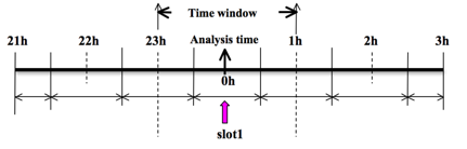
To prepare the observation file, for example, at the analysis time 0h for 3D-Var, all the observations between ±1h (or ±1.5h) will be processed, as illustrated in following figure, which means that the observations between 23h and 1h are treated as the observations at 0h.

Before running obsproc.exe, create the required namelist file namelist.obsproc (see WRFDA/var/obsproc/README.namelist, or the section Description of Namelist Variables for details).

For your reference, an example file named “namelist_obsproc.3dvar.wrfvar-tut” has already been created in the var/obsproc directory. Thus, proceed as follows.

> cp namelist.obsproc.3dvar.wrfvar-tut namelist.obsproc

Next, edit the namelist file namelist.obsproc by changing the following variables to accommodate your experiments.

obs_gts_filename='obs.2008020512'

time_window_min = '2008-02-05_11:00:00',: The earliest time edge as ccyy-mm-dd_hh:mn:ss

time_analysis = '2008-02-05_12:00:00', : The analysis time as ccyy-mm-dd_hh:mn:ss

time_window_max = '2008-02-05_13:00:00',: The latest time edge as ccyy-mm-dd_hh:mn:ss

use_for = '3DVAR', ; used for 3D-Var, default

To run OBSPROC, type

            > obsproc.exe >&! obsproc.out

Once obsproc.exe has completed successfully, you will see an observation data file, obs_gts_2008-02-05_12:00:00.3DVAR, in the obsproc directory. This is the input observation file to WRF-Var.

obs_gts_2008-02-05_12:00:00.3DVAR is an ASCII file that contains a header section (listed below) followed by observations. The meanings and format of observations in the file are described in the last six lines of the header section.

TOTAL = 9066, MISS. =-888888.,

SYNOP = 757, METAR = 2416, SHIP = 145, BUOY = 250, BOGUS = 0, TEMP = 86,

AMDAR = 19, AIREP = 205, TAMDAR= 0, PILOT = 85, SATEM = 106, SATOB = 2556,

GPSPW = 187, GPSZD = 0, GPSRF = 3, GPSEP = 0, SSMT1 = 0, SSMT2 = 0,

TOVS = 0, QSCAT = 2190, PROFL = 61, AIRSR = 0, OTHER = 0,

PHIC = 40.00, XLONC = -95.00, TRUE1 = 30.00, TRUE2 = 60.00, XIM11 = 1.00, XJM11 = 1.00,

base_temp= 290.00, base_lapse= 50.00, PTOP = 1000., base_pres=100000., base_tropo_pres= 20000., base_strat_temp= 215.,

IXC = 60, JXC = 90, IPROJ = 1, IDD = 1, MAXNES= 1,

NESTIX= 60,

NESTJX= 90,

NUMC = 1,

DIS = 60.00,

NESTI = 1,

NESTJ = 1,

INFO = PLATFORM, DATE, NAME, LEVELS, LATITUDE, LONGITUDE, ELEVATION, ID.

SRFC = SLP, PW (DATA,QC,ERROR).

EACH = PRES, SPEED, DIR, HEIGHT, TEMP, DEW PT, HUMID (DATA,QC,ERROR)*LEVELS.

INFO_FMT = (A12,1X,A19,1X,A40,1X,I6,3(F12.3,11X),6X,A40)

SRFC_FMT = (F12.3,I4,F7.2,F12.3,I4,F7.3)

EACH_FMT = (3(F12.3,I4,F7.2),11X,3(F12.3,I4,F7.2),11X,3(F12.3,I4,F7.2))

#------------------------------------------------------------------------------#

…… observations ………

Before running WRF-Var, you may like to learn more about various types of data that will be passed to WRF-Var for this case, for example, their geographical distribution, etc. This file is in ASCII format and so you can easily view it. To have a graphical view about the content of this file, there is a “MAP_plot” utility to look at the data distribution for each type of observations. To use this utility, proceed as follows.

> cd MAP_plot

> make

We have prepared some configure.user.ibm/linux/mac/… files for some platforms, when “make” is typed, the Makefile will use one of them to determine the compiler and compiler option. Please modify the Makefile and configure.user.xxx to accommodate the complier on your platform. Successful compilation will produce Map.exe. Note: The successful compilation of Map.exe requires pre-installed NCARG Graphics libraries under $(NCARG_ROOT)/lib.

Modify the script Map.csh to set the time window and full path of input observation file (obs_gts_2008-02-05_12:00:00.3DVAR). You will need to set the following strings in this script as follows:

Map_plot = /users/noname/WRFDA/var/obsproc/MAP_plot

TIME_WINDOW_MIN = ‘2008020511’

     TIME_ANALYSIS = ‘2008020512’

     TIME_WINDOW_MAX = ‘2008020513’
      OBSDATA = ../obs_gts_2008-02-05_12:00:00.3DVAR

Next, type  

> Map.csh

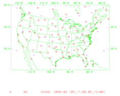
When the job has completed, you will have a gmeta file gmeta.{analysis_time} corresponding to analysis_time=2008020512. This contains plots of data distribution for each type of observations contained in the OBS data file: obs_gts_2008-02-05_12:00:00.3DVAR. To view this, type        

> idt gmeta.2008020512

It will display (panel by panel) geographical distribution of various types of data. Following is the geographic distribution of “sonde” observations for this case.

There is an alternative way to plot the observation by using ncl script: WRFDA/var/graphics/ncl/plot_ob_ascii_loc.ncl. However, with this way, you need to provide the first guess file to the ncl script, and have ncl installed in your system.

 

b. Prepare observational data for 4D-Var

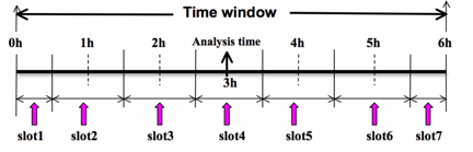
To prepare the observation file, for example, at the analysis time 0h for 4D-Var, all observations from 0h to 6h will be processed and grouped in 7 sub-windows from slot1 to slot7, as illustrated in following figure. NOTE: The “Analysis time” in the figure below is not the actual analysis time (0h), it just indicates the time_analysis setting in the namelist file, and is set to three hours later than the actual analysis time. The actual analysis time is still 0h.

 

An example file named “namelist_obsproc.4dvar.wrfvar-tut” has already been created in the var/obsproc directory. Thus, proceed as follows:

> cp namelist.obsproc.4dvar.wrfvar-tut namelist.obsproc

In the namelist file, you need to change the following variables to accommodate your experiments. In this test case, the actual analysis time is 2008-02-05_12:00:00, but in namelist, the time_analysis should be set to 3 hours later. The different value of time_analysis will make the different number of time slots before and after time_analysis. For example, if you set time_analysis = 2008-02-05_16:00:00, and set the num_slots_past = 4 and time_slots_ahead=2. The final results will be same as before.

obs_gts_filename='obs.2008020512'

time_window_min = '2008-02-05_12:00:00',: The earliest time edge as ccyy-mm-dd_hh:mn:ss

time_analysis = '2008-02-05_15:00:00', : The analysis time as ccyy-mm-dd_hh:mn:ss

time_window_max = '2008-02-05_18:00:00',: The latest time edge as ccyy-mm-dd_hh:mn:ss

use_for = '4DVAR', ; used for 3D-Var, default

; num_slots_past and num_slots_ahead are used ONLY for FGAT and 4DVAR:

num_slots_past = 3, ; the number of time slots before time_analysis

num_slots_ahead = 3, ; the number of time slots after time_analysis

 

To run OBSPROC, type

            > obsproc.exe >&! obsproc.out

Once obsproc.exe has completed successfully, you will see 7 observation data files:

obs_gts_2008-02-05_12:00:00.4DVAR

obs_gts_2008-02-05_13:00:00.4DVAR

obs_gts_2008-02-05_14:00:00.4DVAR

obs_gts_2008-02-05_15:00:00.4DVAR

obs_gts_2008-02-05_16:00:00.4DVAR

obs_gts_2008-02-05_17:00:00.4DVAR

obs_gts_2008-02-05_18:00:00.4DVAR

They are the input observation files to WRF-4DVar. You can also use “MAP_Plot” to view the geographic distribution of different observations at different time slots.

 

Running WRF-Var

a. Download Test Data

The WRF-Var system requires three input files to run: a) A WRF first guess/boudary input format files output from either WPS/real (cold-start) or WRF (warm-start), b) Observations (in ASCII format, PREBUFR or BUFR for radiance), and c) A background error statistics file (containing background error covariance).

The following table summarizes the above info:

In the test case, you will store data in a directory defined by the environment variable $DAT_DIR. This directory can be at any location and it should have read access.  Type

            > setenv DAT_DIR your_choice_of_dat_dir

Here, "your_choice_of_dat_dir" is the directory where the WRF-Var input data is stored. Create this directory if it does not exist, and type

            > cd $DAT_DIR

Download the test data for a “Tutorial” case valid at 12 UTC 5^th February 2008 from http://www.mmm.ucar.edu/wrf/users/wrfda/download/testdata.html

Once you have downloaded “WRFV3.1-Var-testdata.tar.gz” file to $DAT_DIR, extract it by typing

            > gunzip WRFV3.1-Var-testdata.tar.gz
      > tar -xvf WRFV3.1-Var-testdata.tar

Now you should find the following three sub-directories/files under “$DAT_DIR”

ob/2008020512/ob.2008020512.gz # Observation data in “little_r” format
rc/2008020512/wrfinput_d01   # First guess file
rc/2008020512/wrfbdy_d01     # lateral boundary file
be/be.dat                    # Background error file

......

You should first go through the section “Running Observation Preprocessor (OBSPROC)” and have a WRF-3DVar-ready observation file (obs_gts_2008-02-05_12:00:00.3DVAR) generated in your OBSPROC working directory. You could then copy or move obs_gts_2008-02-05_12:00:00.3DVAR to be in $DAT_DIR/ob/2008020512/ob.ascii.

If you want to try 4D-Var, please go through the section “Running Observation Preprocessor (OBSPROC)” and have the WRF-4DVar-ready observation files (obs_gts_2008-02-05_12:00:00.4DVAR,……). You could copy or move the observation files to $DAT_DIR/ob using following commands:

> mv obs_gts_2008-02-05_12:00:00.4DVAR $DAT_DIR/ob/2008020512/ob.ascii+

> mv obs_gts_2008-02-05_13:00:00.4DVAR $DAT_DIR/ob/2008020513/ob.ascii

> mv obs_gts_2008-02-05_14:00:00.4DVAR $DAT_DIR/ob/2008020514/ob.ascii

> mv obs_gts_2008-02-05_15:00:00.4DVAR $DAT_DIR/ob/2008020515/ob.ascii

> mv obs_gts_2008-02-05_16:00:00.4DVAR $DAT_DIR/ob/2008020516/ob.ascii

> mv obs_gts_2008-02-05_17:00:00.4DVAR $DAT_DIR/ob/2008020517/ob.ascii

> mv obs_gts_2008-02-05_18:00:00.4DVAR $DAT_DIR/ob/2008020518/ob.ascii-

At this pont you have three of the input files (first guess, observation and background error statistics files in directory $DAT_DIR) required to run WRF-Var, and have successfully downloaded and compiled the WRF-Var code. If this is correct, we are ready to learn how to run WRF-Var.

b. Run the Case—3D-Var

The data for this case is valid at 12 UTC 5^th February 2008. The first guess comes from the NCEP global final analysis system (FNL), passed through the WRF-WPS and real programs.

To run WRF-3D-Var, first create and cd to a working directory, for example, WRFDA/var/test/tutorial, and then follow the steps below:

> cd WRFDA/var/test/tutorial

> ln -sf WRFDA/run/LANDUSE.TBL ./LANDUSE.TBL

> ln -sf $DAT_DIR/rc/2008020512/wrfinput_d01 ./fg (link first guess file as fg)

> ln -sf WRFDA/var/obsproc/obs_gts_2008-02-05_12:00:00.3DVAR ./ob.ascii (link OBSPROC processed observation file as ob.ascii)

> ln -sf $DAT_DIR/be/be.dat ./be.dat (link background error statistics as be.dat)

> ln -sf WRFDA/var/da/da_wrfvar.exe ./da_wrfvar.exe (link executable)

We will begin by editing the file, namelist.input, which is a very basic namelist.input for running the tutorial test case is shown below and provided as WRFDA/var/test/tutorial/namelist.input. Only the time and domain settings need to be specified in this case, if we are using the default settings provided in WRFDA/Registry/Registry.wrfvar)

&wrfvar1

print_detail_grad=false,
/
&wrfvar2
/

&wrfvar3

/

&wrfvar4

/

&wrfvar5

/

&wrfvar6

/

&wrfvar7

/

&wrfvar8

/

&wrfvar9

/

&wrfvar10

/

&wrfvar11

/

&wrfvar12

/

&wrfvar13

/

&wrfvar14

/

&wrfvar15

/

&wrfvar16

/

&wrfvar17

/

&wrfvar18

analysis_date="2008-02-05_12:00:00.0000",

/

&wrfvar19

/

&wrfvar20

/

&wrfvar21

time_window_min="2008-02-05_11:00:00.0000",

/

&wrfvar22

time_window_max="2008-02-05_13:00:00.0000",

/

&wrfvar23

/

&time_control

start_year=2008,

start_month=02,

start_day=05,

start_hour=12,

end_year=2008,

end_month=02,

end_day=05,

end_hour=12,

/

&dfi_control

/

&domains

e_we=90,

e_sn=60,

e_vert=41,

dx=60000,

dy=60000,

/

&physics

mp_physics=3,

ra_lw_physics=1,

ra_sw_physics=1,

radt=60,

sf_sfclay_physics=1,

sf_surface_physics=1,

bl_pbl_physics=1,

cu_physics=1,

cudt=5,

num_soil_layers=5, (IMPORTANT: it’s essential to make sure the setting here is consistent with the number in your first guess file)

mp_zero_out=2,

co2tf=0,

/

&fdda

/

&dynamics

/

&bdy_control

/

&grib2

/

&namelist_quilt

/

> da_wrfvar.exe >&! wrfda.log

The file wrfda.log (or rsl.out.0000 if running in distributed-memory mode) contains important WRF-Var runtime log information. Always check the log after a WRF-Var run:

*** VARIATIONAL ANALYSIS ***

DYNAMICS OPTION: Eulerian Mass Coordinate

WRF NUMBER OF TILES = 1

Set up observations (ob)

Using ASCII format observation input

scan obs ascii

end scan obs ascii

Observation summary

ob time 1

sound 85 global, 85 local

synop 531 global, 525 local

pilot 84 global, 84 local

satem 78 global, 78 local

geoamv 736 global, 719 local

polaramv 0 global, 0 local

airep 132 global, 131 local

gpspw 183 global, 183 local

gpsrf 0 global, 0 local

metar 1043 global, 1037 local

ships 86 global, 82 local

ssmi_rv 0 global, 0 local

ssmi_tb 0 global, 0 local

ssmt1 0 global, 0 local

ssmt2 0 global, 0 local

qscat 0 global, 0 local

profiler 61 global, 61 local

buoy 216 global, 216 local

bogus 0 global, 0 local

pseudo 0 global, 0 local

radar 0 global, 0 local

radiance 0 global, 0 local

airs retrieval 0 global, 0 local

sonde_sfc 85 global, 85 local

mtgirs 0 global, 0 local

tamdar 0 global, 0 local

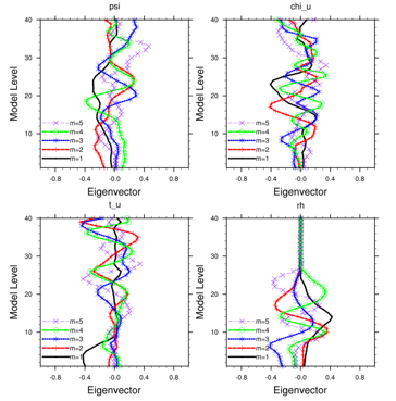
Set up background errors for regional application

WRF-Var dry control variables are:psi, chi_u, t_u and psfc

Humidity control variable is q/qsg

Using the averaged regression coefficients for unbalanced part

Vertical truncation for psi = 15( 99.00%)

Vertical truncation for chi_u = 20( 99.00%)

Vertical truncation for t_u = 29( 99.00%)

Vertical truncation for rh = 22( 99.00%)

Calculate innovation vector(iv)

Minimize cost function using CG method

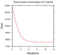
For this run cost function diagnostics will not be written

Starting outer iteration : 1

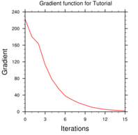
Starting cost function: 2.28356084D+04, Gradient= 2.23656955D+02

For this outer iteration gradient target is: 2.23656955D+00

----------------------------------------------------------

Iter Gradient Step

1 1.82455068D+02 7.47025772D-02

2 1.64971618D+02 8.05531077D-02

3 1.13694365D+02 7.22382618D-02

4 7.87359568D+01 7.51905761D-02

5 5.71607218D+01 7.94572516D-02

6 4.18746777D+01 8.30731280D-02

7 2.95722963D+01 6.13223951D-02

8 2.34205172D+01 9.05920463D-02

9 1.63772518D+01 6.48090044D-02

10 1.09735524D+01 7.71148550D-02

11 8.22748934D+00 8.81041046D-02

12 5.65846963D+00 7.89528133D-02

13 4.15664769D+00 7.45589721D-02

14 3.16925808D+00 8.35300020D-02

----------------------------------------------------------

Inner iteration stopped after 15 iterations

Final: 15 iter, J= 1.76436785D+04, g= 2.06098421D+00

----------------------------------------------------------

Diagnostics

Final cost function J = 17643.68

 

Total number of obs. = 26726

Final value of J = 17643.67853

Final value of Jo = 15284.64894

Final value of Jb = 2359.02958

Final value of Jc = 0.00000

Final value of Je = 0.00000

Final value of Jp = 0.00000

Final J / total num_obs = 0.66017

Jb factor used(1) = 1.00000

Jb factor used(2) = 1.00000

Jb factor used(3) = 1.00000

Jb factor used(4) = 1.00000

Jb factor used(5) = 1.00000

Jb factor used = 1.00000

Je factor used = 1.00000

VarBC factor used = 1.00000

 

*** WRF-Var completed successfully ***

 

 

A file called namelist.output (which contains the complete namelist settings) will be generated after a successful da_wrfvar.exe run. Those settings that appear in namelist.output that are not specified in your namelist.input are the default values from WRFDA/Registry/Registry.wrfvar.

After successful completion of job, wrfvar_output (the WRF-Var analysis file, i.e. the new initial condition for WRF) should appear in the working directory along with a number of diagnostic files. Various text diagnostics output files will be explained in the next section (WRF-Var Diagnostics).

In order to understand the role of various important WRF-Var options, try re-running WRF-Var by changing different namelist options. Such as making WRF-Var convergence criteria more stringent. This is achieved by reducing the value of the convergence criteria “EPS” to e.g. 0.0001 by adding "EPS=0.0001" in the namelist.input record &wrfvar6. See section (WRF-Var additional exercises) for more namelist options

b. Run the Case—4D-Var

To run WRF-4DVar, first create and cd to a working directory, for example, WRFDA/var/test/4dvar; next assuming that we are using the C-shell, set the working directories for the three WRF-4DVar components WRFDA, WRFNL and WRFPLUS thusly

> setenv WRFDA_DIR /ptmp/$user/WRFDA

> setenv WRFNL_DIR /ptmp/$user/WRFNL

> setenv WRFPLUS_DIR /ptmp/$user/WRFPLUS

Assume the analysis date is 2008020512 and the test data directories are:

> setenv DATA_DIR /ptmp/$user/DATA

> ls –lr $DATA_DIR

ob/2008020512

ob/2008020513

ob/2008020514

ob/2008020515

ob/2008020516

ob/2008020517

ob/2008020518

rc/2008020512

be

Note: Currently, WRF-4DVar can only run with the observation data processed by OBSPROC, and cannot work with PREPBUFR format data; Although WRF-4DVar is able to assimilate satellite radiance BUFR data, but this capability is still under testing.

Assume the working directory is:

> setenv WORK_DIR $WRFDA_DIR/var/test/4dvar

Then follow the steps below:

1) Link the executables.

> cd $WORK_DIR

> ln -fs $WRFDA_DIR/var/da/da_wrfvar.exe .

> cd $WORK_DIR/nl

> ln -fs $WRFNL_DIR/main/wrf.exe .

> cd $WORK_DIR/ad

> ln -fs $WRFPLUS_DIR/main/wrfplus.exe .

> cd $WORK_DIR/tl

> ln -fs $WRFPLUS_DIR/main/wrfplus.exe .

2) Link the observational data, first guess and BE. (Currently, only LITTLE_R formatted observational data is supported in 4D-Var, PREPBUFR observational data is not supported)

> cd $WORK_DIR

> ln -fs $DATA_DIR/ob/2008020512/ob.ascii+ ob01.ascii

> ln -fs $DATA_DIR/ob/2008020513/ob.ascii ob02.ascii

> ln -fs $DATA_DIR/ob/2008020514/ob.ascii ob03.ascii

> ln -fs $DATA_DIR/ob/2008020515/ob.ascii ob04.ascii

> ln -fs $DATA_DIR/ob/2008020516/ob.ascii ob05.ascii

> ln -fs $DATA_DIR/ob/2008020517/ob.ascii ob06.ascii

> ln -fs $DATA_DIR/ob/2008020518/ob.ascii- ob07.ascii

 

> ln -fs $DATA_DIR/rc/2008020512/wrfinput_d01 .

> ln -fs $DATA_DIR/rc/2008020512/wrfbdy_d01 .

> ln -fs wrfinput_d01 fg

> ln -fs wrfinput_d01 fg01

 

> ln -fs $DATA_DIR/be/be.dat .

 

3) Establish the miscellaneous links.

> cd $WORK_DIR

> ln -fs nl/nl_d01_2008-02-05_13:00:00 fg02

> ln -fs nl/nl_d01_2008-02-05_14:00:00 fg03

> ln -fs nl/nl_d01_2008-02-05_15:00:00 fg04

> ln -fs nl/nl_d01_2008-02-05_16:00:00 fg05

> ln -fs nl/nl_d01_2008-02-05_17:00:00 fg06

> ln -fs nl/nl_d01_2008-02-05_18:00:00 fg07

 

> ln -fs ad/ad_d01_2008-02-05_12:00:00 gr01

 

> ln -fs tl/tl_d01_2008-02-05_13:00:00 tl02

> ln -fs tl/tl_d01_2008-02-05_14:00:00 tl03

> ln -fs tl/tl_d01_2008-02-05_15:00:00 tl04

> ln -fs tl/tl_d01_2008-02-05_16:00:00 tl05

> ln -fs tl/tl_d01_2008-02-05_17:00:00 tl06

> ln -fs tl/tl_d01_2008-02-05_18:00:00 tl07

 

> cd $WORK_DIR/ad

> ln -fs ../af01 auxinput3_d01_2008-02-05_12:00:00

> ln -fs ../af02 auxinput3_d01_2008-02-05_13:00:00

> ln -fs ../af03 auxinput3_d01_2008-02-05_14:00:00

> ln -fs ../af04 auxinput3_d01_2008-02-05_15:00:00

> ln -fs ../af05 auxinput3_d01_2008-02-05_16:00:00

> ln -fs ../af06 auxinput3_d01_2008-02-05_17:00:00

> ln -fs ../af07 auxinput3_d01_2008-02-05_18:00:00

4) Run in single processor mode (serial compilation required for WRFDA, WRFNL and WRFPLUS)

         Edit $WORK_DIR/namelist.input to match your experiment settings.

         > cp $WORK_DIR/nl/namelist.input.serial $WORK_DIR/nl/namelist.input

         Edit $WORK_DIR/nl/namelist.input to match your experiment settings.

         > cp $WORK_DIR/ad/namelist.input.serial $WORK_DIR/ad/namelist.input

         > cp $WORK_DIR/tl/namelist.input.serial $WORK_DIR/tl/namelist.input

         Edit $WORK_DIR/ad/namelist.input and $WORK_DIR/tl/namelist.input to match your experiment settings, but only change following variables:

&time_control

run_hours=06,

start_year=2008,

start_month=02,

start_day=05,

start_hour=12,

end_year=2008,

end_month=02,

end_day=05,

end_hour=18,

......

&domains

time_step=360, # NOTE:MUST BE THE SAME WITH WHICH IN $WORK_DIR/nl/namelist.input

e_we=90,

e_sn=60,

e_vert=41,

dx=60000,

dy=60000,

......

 

> cd $WORK_DIR

> setenv NUM_PROCS 1

> ./da_wrfvar.exe >&! wrfda.log

5) Run with multiple processors with MPMD mode. (dmpar compilation required for WRFDA, WRFNL and WRFPLUS)

         Edit $WORK_DIR/namelist.input to match your experiment settings.

         > cp $WORK_DIR/nl/namelist.input.parallel $WORK_DIR/nl/namelist.input

         Edit $WORK_DIR/nl/namelist.input to match your experiment settings.

         > cp $WORK_DIR/ad/namelist.input.parallel $WORK_DIR/ad/namelist.input

         > cp $WORK_DIR/tl/namelist.input.parallel $WORK_DIR/tl/namelist.input

         Edit $WORK_DIR/ad/namelist.input and $WORK_DIR/tl/namelist.input to match your experiment settings.

Currently, parallel WRF 4D-Var is a MPMD (Multiple Program Multiple Data) application. Because there are so many parallel configurations across the platforms, it is very difficult to define a generic way to run the WRF 4D-Var parallel. As an example, to launch the three WRF 4D-Var executables as a concurrent parallel job on a 16 processor cluster, use:

> mpirun –np 4 da_wrfvar.exe: -np 8 ad/wrfplus.exe: -np 4 nl/wrf.exe

In the above example, 4 processors are assigned to run WRFDA, 4 processors are assigned to run WRFNL and 8 processors for WRFPLUS due to high computational cost in adjoint code.

The file wrfda.log (or rsl.out.0000 if running in parallel mode) contains important WRF-4DVar runtime log information. Always check the log after a WRF-4DVar run.

 

Radiance Data Assimilations in WRF-Var

This section gives brief description for various aspects related to radiance assimilation in WRF-Var. Each aspect is described mainly from the viewpoint of usage rather than more technical and scientific details, which will appear in separated technical report and scientific paper. Namelist parameters controlling different aspects of radiance assimilation will be detailed in the following sections. . It should be noted that this section does not cover general aspects of the WRF-Var assimilation. These can be found in other sections of chapter 6 of this users guide or other WRF-Var documentation.

 

a. Running WRF-Var with radiances

 

In addition to the basic input files (LANDUSE.TBL, fg, ob.ascii, be.dat) mentioned in “Running WRF-Var” section, the following extra files are required for radiances: radiance data in NCEP BUFR format, radiance_info files, VARBC.in, RTM (CRTM or RTTOV) coefficient files.

 

Edit namelist.input (Pay special attention to &wrfvar4, &wrfvar14, &wrfvar21, and &wrfvar22 for radiance-related options)

> ln -sf ${DAT_DIR}/gdas1.t00z.1bamua.tm00.bufr_d ./amsua.bufr

> ln -sf ${DAT_DIR}/gdas1.t00z.1bamub.tm00.bufr_d ./amsub.bufr

> ln -sf WRFDA/var/run/radiance_info ./radiance_info # (radiance_info is a directory)

> ln -sf WRFDA/var/run/VARBC.in ./VARBC.in

(CRTM only) > ln -sf REL-1.2.JCSDA_CRTM/crtm_coeffs ./crtm_coeffs #(crtm_coeffs is a directory)

(RTTOV only) > ln -sf rttov87/rtcoef_rttov7/* . # (a list of rtcoef* files)

 

See the following sections for more details on each aspect.

 

b. Radiance Data Ingest

 

Currently, the ingest interface for NCEP BUFR radiance data is implemented in WRF-Var. The radiance data are available through NCEP’s public ftp server ftp://ftp.ncep.noaa.gov/pub/data/nccf/com/gfs/prod/gdas.${yyyymmddhh} in near real-time (with 6-hour delay) and can meet requirements both for research purposes and some real-time applications.

 

So far, WRF-Var can read data from the NOAA ATOVS instruments (HIRS, AMSU-A, AMSU-B and MHS), the EOS Aqua instruments (AIRS, AMSU-A) and DMSP instruments (SSMIS). Note that NCEP radiance BUFR files are separated by instrument names (i.e., each file for one type instrument) and each file contains global radiance (generally converted to brightness temperature) within 6-hour assimilation window from multi-platforms. For running WRF-Var, users need to rename NCEP corresponding BUFR files (table 1) to hirs3.bufr (including HIRS data from NOAA-15/16/17), hirs4.bufr (including HIRS data from NOAA-18, METOP-2), amsua.bufr (including AMSU-A data from NOAA-15/16/18, METOP-2), amsub.bufr (including AMSU-B data from NOAA-15/16/17), mhs.bufr (including MHS data from NOAA-18 and METOP-2), airs.bufr (including AIRS and AMSU-A data from EOS-AQUA) and ssmis.bufr (SSMIS data from DMSP-16, AFWA provided) for WRF-Var filename convention. Note that airs.bufr file contains not only AIRS data but also AMSU-A, which is collocated with AIRS pixels (1 AMSU-A pixels collocated with 9 AIRS pixels). Users must place these files in the working directory where WRF-Var executable is located. It should also be mentioned that WRF-Var reads these BUFR radiance files directly without use if any separate pre-processing program is used. All processing of radiance data, such as quality control, thinning and bias correction and so on, is carried out inside WRF-Var. This is different from conventional observation assimilation, which requires a pre-processing package (OBSPROC) to generate WRF-Var readable ASCII files. For reading the radiance BUFR files, WRF-Var must be compiled with the NCEP BUFR library (see http://www.nco.ncep.noaa.gov/sib/decoders/BUFRLIB/ ).

 

Table 1: NCEP and WRF-Var radiance BUFR file naming convention

 

Namelist parameters are used to control the reading of corresponding BUFR files into WRF-Var. For instance, USE_AMSUAOBS, USE_AMSUBOBS, USE_HIRS3OBS, USE_HIRS4OBS, USE_MHSOBS, USE_AIRSOBS, USE_EOS_AMSUAOBS and USE_SSMISOBS control whether or not the respective file is read. These are logical parameters that are assigned to FALSE by default; therefore they must be set to true to read the respective observation file. Also note that these parameters only control whether the data is read, not whether the data included in the files is to be assimilated. This is controlled by other namelist parameters explained in the next section.

 

NCEP BUFR files downloaded from NCEP’s public ftp server ftp://ftp.ncep.noaa.gov/pub/data/nccf/com/gfs/prod/gdas.${yyyymmddhh} are Fortran-blocked on big-endian machine and can be directly used on big-endian machines (for example, IBM). For most Linux clusters with Intel platforms, users need to first unblock the BUFR files, and then reblock them. The utility for blocking/unblocking is available from http://www.nco.ncep.noaa.gov/sib/decoders/BUFRLIB/toc/cwordsh

 

 

c. Radiative Transfer Model

 

The core component for direct radiance assimilation is to incorporate a radiative transfer model (RTM, should be accurate enough yet fast) into the WRF-Var system as one part of observation operators. Two widely used RTMs in NWP community, RTTOV8* (developed by EUMETSAT in Europe), and CRTM (developed by the Joint Center for Satellite Data Assimilation (JCSDA) in US), are already implemented in WRF-Var system with a flexible and consistent user interface. Selecting which RTM to be used is controlled by a simple namelist parameter RTM_OPTION (1 for RTTOV, the default, and 2 for CRTM). WRF-Var is designed to be able to compile with only one of two RTM libraries or without RTM libraries (for those not interested in radiance assimilation) by the definition of environment variables “CRTM” and “RTTOV” (see Installing WRF-Var section).

 

Both RTMs can calculate radiances for almost all available instruments aboard various satellite platforms in orbit. An important feature of WRF-Var design is that all data structures related to radiance assimilation are dynamically allocated during running time according to simple namelist setup. The instruments to be assimilated are controlled at run time by four integer namelist parameters: RTMINIT_NSENSOR (the total number of sensors to be assimilated), RTMINIT_PLATFORM (the platforms IDs array to be assimilated with dimension RTMINIT_NSENSOR, e.g., 1 for NOAA, 9 for EOS, 10 for METOP and 2 for DMSP), RTMINIT_SATID (satellite IDs array) and RTMINIT_SENSOR (sensor IDs array, e.g., 0 for HIRS, 3 for AMSU-A, 4 for AMSU-B, 15 for MHS, 10 for SSMIS, 11 for AIRS). For instance, the configuration for assimilating 12 sensors from 7 satellites (what WRF-Var can assimilated currently) will be

 

RTMINIT_NSENSOR = 12 # 5 AMSUA; 3 AMSUB; 2 MHS; 1 AIRS; 1 SSMIS

RTMINIT_PLATFORM = 1,1,1,9,10, 1,1,1, 1,10, 9, 2

RTMINIT_SATID = 15,16,18,2,2, 15,16,17, 18,2, 2, 16

RTMINIT_SENSOR = 3,3,3,3,3, 4,4,4, 15,15, 11, 10

 

The instrument triplets (platform, satellite and sensor ID) in the namelist can be rank in any order. More detail about the convention of instrument triplet can be found at the tables 2 and 3 in RTTOV8/9 Users Guide (http://www.metoffice.gov.uk/research/interproj/nwpsaf/rtm/rttov8_ug.pdf Or http://www.metoffice.gov.uk/research/interproj/nwpsaf/rtm/rttov9_files/users_guide_91_v1.6.pdf)

 

CRTM uses different instrument naming method. A convert routine inside WRF-Var is already created to make CRTM use the same instrument triplet as RTTOV such that the user interface remains the same for RTTOV and CRTM.

 

When running WRF-Var with radiance assimilation switched on (RTTOV or CRTM), a set of RTM coefficient files need to be loaded. For RTTOV option, RTTOV coefficient files are to be directly copied or linked under the working directory; for CRTM option, CRTM coefficient files are to be copied or linked to a sub-directory “crtm_coeffs” under the working directory. Only coefficients listed in namelist are needed. Potentially WRF-Var can assimilate all sensors as long as the corresponding coefficient files are provided with RTTOV and CRTM. In addition, necessary developments on corresponding data interface, quality control and bias correction are also important to make radiance data assimilated properly. However, a modular design of radiance relevant routines already facilitates much to add more instruments in WRF-Var.

 

RTTOV and CRTM packages are not distributed with WRF-Var due to license and support issues. Users are encouraged to contact the corresponding team for obtaining RTMs. See following links for more information.

http://www.metoffice.gov.uk/research/interproj/nwpsaf/rtm/index.html for RTTOV,

ftp://ftp.emc.ncep.noaa.gov/jcsda/CRTM/ for CRTM.

 

 

d. Channel Selection

 

Channel selection in WRF-Var is controlled by radiance ‘info’ files located in the sub-directory ‘radiance_info’ under the working directory. These files are separated by satellites and sensors, e.g., noaa-15-amsua.info, noaa-16-amsub.info, dmsp-16-ssmis.info and so on. An example for 5 channels from noaa-15-amsub.info is shown below. The fourth column is used by WRF-Var to control if assimilating corresponding channel. Channels with the value “-1” indicates that the channel is “not assimilated” (channels 1, 2 and 4 in this case), with the value “1” means “assimilated” (channels 3 and 5). The sixth column is used by WRF-Var to set the observation error for each channel. Other columns are not used by WRF-Var. It should be mentioned that these error values might not necessarily be optimal for your applications; It is user’s responsibility to obtain the optimal error statistics for your own applications.

 

sensor channel IR/MW use idum varch polarisation(0:vertical;1:horizontal)

415 1 1 -1 0 0.5500000000E+01 0.0000000000E+00

415 2 1 -1 0 0.3750000000E+01 0.0000000000E+00

415 3 1 1 0 0.3500000000E+01 0.0000000000E+00

415 4 1 -1 0 0.3200000000E+01 0.0000000000E+00

415 5 1 1 0 0.2500000000E+01 0.0000000000E+00

 

 

e. Bias Correction

 

Satellite radiance is generally considered biased with respect to a reference (e.g., background or analysis field in NWP assimilation) due to system error of observation itself, reference field and RTM. Bias correction is a necessary step prior to assimilating radiance data. In WRF-Var, there are two ways of performing bias correction. One is based on Harris and Kelly (2001) method and is carried out using a set of coefficient files pre-calculated with an off-line statistics package, which will apply to a training dataset for a month-long period. The other is Variational Bias Correction (VarBC). Only VarBC is introduced here and recommended for users because of its relative simplicity in usage.

f. Variational Bias Correction

 

Getting started with VarBC

To use VarBC, set namelist option USE_VARBC to TRUE and have a VARBC.in file in the working directory. VARBC.in is a VarBC setup file in ASCII format. A template is provided with the WRF-Var package (WRFDA/var/run/VARBC.in).

 

Input and Output files

All VarBC input is passed through one single ASCII file called VARBC.in file. Once WRF-Var has run with the VarBC option switched on, it will produce a VARBC.out file which looks very much like the VARBC.in file you provided. This output file will then be used as input file for the next assimilation cycle.

 

Coldstart

Coldstarting means starting the VarBC from scratch i.e. when you do not know the values of the bias parameters.

 

The Coldstart is a routine in WRF-Var. The bias predictor statistics (mean and standard deviation) are computed automatically and will be used to normalize the bias parameters. All coldstarted bias parameters are set to zero, except the first bias parameter (= simple offset), which is set to the mode (=peak) of the distribution of the (uncorrected) innovations for the given channel.

 

A threshold of number of observations can be set through a namelist option VARBC_NOBSMIN (default = 10), under which it is considered that not enough observations are present to keep the Coldstart values (i.e. bias predictor statistics and bias parameter values) for the next cycle. In this case, the next cycle will do another Coldstart.

 

Background Constraint for the bias parameters

The background constraint controls the inertia you want to impose on the predictors (i.e. the smoothing in the predictor time series). It corresponds to an extra term in the WRF-Var cost function.

 

It is defined through an integer number in the VARBC.in file. This number is related to a number of observations: the bigger the number, the more inertia constraint. If these numbers are set to zero, the predictors can evolve without any constraint.

 

Scaling factor

The VarBC uses a specific preconditioning, which can be scaled through a namelist option VARBC_FACTOR (default = 1.0).

 

Offline bias correction

The analysis of the VarBC parameters can be performed "offline", i.e. independently from the main WRF-Var analysis. No extra code is needed, just set the following MAX_VERT_VAR* namelist variables to be 0, which will disable the standard control variable and only keep the VarBC control variable.

 

MAX_VERT_VAR1=0.0

MAX_VERT_VAR2=0.0

MAX_VERT_VAR3=0.0

MAX_VERT_VAR4=0.0

MAX_VERT_VAR5=0.0

 

Freeze VarBC

In certain circumstances, you might want to keep the VarBC bias parameters constant in time (="frozen"). In this case, the bias correction is read and applied to the innovations, but it is not updated during the minimization. This can easily be achieved by setting the namelist options:

 

USE_VARBC=false

FREEZE_VARBC=true

 

Passive observations

Some observations are useful for preprocessing (e.g. Quality Control, Cloud detection) but you might not want to assimilate them. If you still need to estimate their bias correction, these observations need to go through the VarBC code in the minimization. For this purpose, the VarBC uses a separate threshold on the QC values, called "qc_varbc_bad". This threshold is currently set to the same value as "qc_bad", but can easily be changed to any ad hoc value.

 

g. Other namelist variables to control radiance assimilation

 

RAD_MONITORING (30)       

Integer array of dimension RTMINIT_NSENSER, where 0 for assimilating mode, 1 for monitoring mode (only calculate innovation).

           

THINNING

Logical, TRUE will perform thinning on radiance data.         

 

THINNING_MESH (30)

Real array with dimension RTMINIT_NSENSOR, values indicate thinning mesh (in KM) for different sensors.

           

QC_RAD

Logical, control if perform quality control, always set to TRUE.

           

WRITE_IV_RAD_ASCII

Logical, control if output Observation minus Background files which are in ASCII format and separated by sensors and processors.

           

WRITE_OA_RAD_ASCII

Logical, control if output Observation minus Analysis files (including also O minus B) which are ASCII format and separated by sensors and processors.

           

USE_ERROR_FACTOR_RAD

Logical, controls use of a radiance error tuning factor file “radiance_error.factor”, which is created with empirical values or generated using variational tunning method (Desroziers and Ivanov, 2001)

           

ONLY_SEA_RAD

Logical, controls whether only assimilating radiance over water.       

 

TIME_WINDOW_MIN

String, e.g., "2007-08-15_03:00:00.0000", start time of assimilation time window

 

TIME_WINDOW_MAX

String, e.g., "2007-08-15_09:00:00.0000", end time of assimilation time window

 

CRTM_ATMOSPHERE

Integer, used by CRTM to choose climatology reference profile used above model top (up to 0.01hPa).

0: Invalid (default, use U.S. Standard Atmosphere)

1: Tropical

2: Midlatitude summer

3: Midlatitude winter

4: Subarctic summer

5: Subarctic winter

6: U.S. Standard Atmosphere

 

USE_ANTCORR (30)

Logical array with dimension RTMINIT_NSENSER, control if performing Antenna Correction in CRTM.

 

AIRS_WARMEST_FOV

Logical, controls whether using the observation brightness temperature for AIRS Window channel #914 as criterium for GSI thinning.

 

 

h. Diagnostics and Monitoring

 

(1) Monitoring capability within WRF-Var.

 

Run WRF-Var with the rad_monitoring namelist parameter in record wrfvar14 in namelist.input.

 

0 means assimilating mode, innovations (O minus B) are calculated and data are used in minimization.

1 means monitoring mode: innovations are calculated for diagnostics and monitoring. Data are not used in minimization.

 

Number of rad_monitoring should correspond to number of rtminit_nsensor. If rad_monitoring is not set, then default value of 0 will be used for all sensors.

 

(2) Outputing radiance diagnostics from WRF-Var

 

Run WRF-Var with the following namelist variables in record wrfvar14 in namelist.input.

 

write_iv_rad_ascii=.true.

to write out (observation-background) and other diagnostics information in plain-text files with prefix inv followed by instrument name and processor id. For example, inv_noaa-17-amsub.0000

 

write_oa_rad_ascii=.true.

to write out (observation-background), (observation-analysis) and other diagnostics information in plain-text files with prefix oma followed by instrument name and processor id. For example, oma_noaa-18-mhs.0001

 

Each processor writes out information of one instrument in one file in the WRF-var working directory.

 

(3) Radiance diagnostics data processing

 

A Fortran90 program is used to collect the inv* or oma* files and write out in netCDF format (one instrument in one file with prefix diags followed by instrument name, analysis date, and suffix .nc)) for easier data viewing, handling and plotting with netCDF utilities and NCL scripts.

 

(4) Radiance diagnostics plotting

 

NCL scripts (WRFDA/var/graphics/ncl/plot_rad_diags.ncl and WRFDA/var/graphics/ncl/advance_cymdh.ncl) are used for plotting. The NCL script can be run from a shell script, or run stand-alone with interactive ncl command (need to edit the NCL script and set the plot options. Also the path of advance_cymdh.ncl, a date advancing script loaded in the main NCL plotting script, may need to be modified).

 

Step (3) and (4) can be done by running a single ksh script (WRFDA/var/scripts/da_rad_diags.ksh) with proper settings. In addition to the settings of directories and what instruments to plot, there are some useful plotting options, explained below.

 

 

 

(5) evolution of VarBC parameters

 

NCL scripts (WRFDA/var/graphics/ncl/plot_rad_varbc_param.ncl and WRFDA/var/graphics/ncl/advance_cymdh.ncl) are used for plotting evolutions of VarBC parameters.

 

WRF-Var Diagnostics

WRF-Var produces a number of diagnostic files that contain useful information on how the data assimilation has performed. This section will introduce you to some of these files, and what to look for.

Having run WRF-Var, it is important to check a number of output files to see if the assimilation appears sensible. The WRF-Var package, which includes lots of useful scripts may be downloaded from http://www.mmm.ucar.edu/wrf/users/wrfda/download/tools.html

The content of some useful diagnostic files are as follows:

cost_fn and grad_fn: These files hold (in ASCII format) WRF-Var cost and gradient function values, respectively, for the first and last iterations. However, if you run with PRINT_DETAIL_GRAD=true, these values will be listed for each iteration; this can be helpful for visualization purposes. The NCL script WRFDA/var/graphcs/ncl/plot_cost_grad_fn.ncl may be used to plot the content of cost_fn and grad_fn, if these files are generated with PRINT_DETAIL_GRAD=true.

Note: Make sure that you removed first two lines (header) in cost_fn and grad_fn before you plot. Also you need to specify the directory name for these two files.

gts_omb_oma_01: It contains (in ASCII format) information on all of the observations used by the WRF-Var run. Each observation has its observed value, quality flag, observation error, observation minus background (OMB), and observation minus analysis (OMA). This information is very useful for both analysis and forecasts verification purposes.

namelist.input: This is the WRF-Var input namelist file, which contains all the user defined non-default options. Any namelist defined options that do not appear in this file, should have their names checked against values in WRFDA/Registry/Registry.wrfvar.

namelist.output: A consolidated list of all the namelist options used.

rsl*: Files containing information of standard WRF-Var output from individual processors when multiple processors are used. It contains host of information on number of observations, minimization, timings etc. Additional diagnostics may be printed in these files by including various “print” WRF-Var namelist options. To learn more about these additional “print” options, search “print_” string in WRFDA/Registry/Registry.wrfvar.

statistics: Text file containing OMB (OI), OMA (OA) statistics (minimum, maximum, mean and standard deviation) for each observation type and variable. This information is very useful in diagnosing how WRF-Var has used different components of the observing system. Also contained are the analysis minus background (A-B) statistics i.e. statistics of the analysis increments for each model variable at each model level. This information is very useful in checking the range of analysis increment values found in the analysis, and where they are in the WRF-model grid space.

The WRF-Var analysis file is wrfvar_output. It is in WRF (NetCDF) format. It will become the input file “wrfinput_d01” of any subsequent WRF runs after lateral boundary and/or low boundary conditions are updated by another WRF-Var utility (See section “Updating WRF boundary conditions”).

A NCL script WRFDA/var/graphics/ncl/WRF-Var_plot.ncl, is provided for plotting. You need to specify the analsyis_file name, its full path etc. Please see the in-line comments in the script for details.

As an example, if you are aiming to display U-component of the analysis at level 18, execute following command after modifying the script “WRFDA/var/graphcs/ncl/WRF-Var_plot.ncl”, make sure following piece of codes are uncommented:

var = "U"

fg = first_guess->U

an = analysis->U

plot_data = an

When you execute the following command from WRFDA/var/graphics/ncl.

           > ncl WRF-Var_plot.ncl

The plot should look like:

You may change the variable name, level etc in this script to display the variable of your choice at the desired eta level.

Take time to look through the text output files to ensure you understand how WRF-Var has performed. For example,

How closely has WRF-Var fitted individual observation types? Look at the statistics file to compare the O-B and O-A statistics.

How big are the analysis increments? Again, look in the statistics file to see minimum/maximum values of A-B for each variable at various levels. It will give you a feel of the impact of input observation data you assimilated via WRF-Var by modifying the input analysis first guess.

How long did WRF-Var take to converge? Does it really converge? You will get the answers of all these questions by looking into rsl-files, as it indicates the number of iterations taken by WRF-Var to converge. If this is the same as the maximum number of iterations specified in the namelist (NTMAX) or its default value (=200) set in WRFDA/Registry/Registry.wrfvar, then it means that the analysis solution did not converge. If so, you may like to increase the value of “NTMAX” and rerun your case to ensure that the convergence is achieved. On the other hand, a normal WRF-Var run should usually converge within 100 iterations. If it still doesn’t converge in 200 iterations, that means there might be some problem in the observations or first guess.

A good visual way of seeing the impact of assimilation of observations is to plot the analysis increments (i.e. analysis minus first guess difference). There are many different graphics packages used (e.g. RIP4, NCL, GRADS etc) that can do this. The plot of level 18 theta increments below was produced using the particular NCL script. This script is located at WRFDA/var/graphcs/ncl/WRF-Var_plot.ncl.

You need to modify this script to fix the full path for first_guess & analysis files. You may also like to modify the display level by setting “kl” and the name of the variable to display by setting “var”. Further details are given in this script.

If you are aiming to display increment of potential temperature at level 18, after modifying WRFDA/var/graphcs/ncl/WRF-Var_plot.ncl suitably, make sure following pieces of codes are uncommented:

var = "T"

fg = first_guess->T ;Theta- 300

an = analysis->T ;Theta- 300

plot_data = an - fg

When you execute the following command from “WRFDA/var/graphics/ncl”.

> ncl WRF-Var_plot.ncl

The plot created will looks as follows:

Note: Larger analysis increments indicate a larger data impact in the corresponding region of the domain.

 

Updating WRF boundary conditions

Before running NWP forecast using WRF-model with WRF-Var analysis, the values and tendencies for each of predicted variables for the first time period in the lateral boundary condition file for domain-1 (wrfbdy_d01) must be updated to be consistent with the new WRF-Var initial condition (analysis). This is absolutely essential. Moreover, in the cycling run mode (warm-start), the low boundary in the WRF-Var anaylsis file also need to be updated based on the information of the wrfinput file generated by WPS/real.exe at the analysis time. So there are three input files: WRF-Var analysis, wrfinput and wrfbdy files from WPS/real.exe, and a namelist file: param.in for running da_update_bc.exe for domain-1.

For the nested domains, domain-2, domain-3…, the lateral boundaries are provided by their parent domains, so no lateral boundary update needed for these domains, But the low boundaries in each of the nested domains’ WRF-Var analysis files are still need to be updated. In these cases, you must set the namelist variable, domain_id > 1 (default is 1 for domain-1), and no wrfbdy_d01file need to be provided to the namelist variable: wrf_bdy_file.

This procedure is performed by the WRF-Var utility called da_updated_bc.exe.

Note: Make sure that you have da_update_bc.exe in WRFDA/var/build directory. This executable should be created when you compiled WRF-Var code,

To run da_update_bc.exe, follow the steps below:

> cd WRFDA/var/test/update_bc

> cp –p $DAT_DIR/rc/2008020512/wrfbdy_d01 ./wrfbdy_d01 (IMPORTANT: make a copy of wrfbdy_d01 as the wrf_bdy_file will be overwritten by da_update_bc.exe)

> vi parame.in

&control_param

wrfvar_output_file = './wrfvar_output'

wrf_bdy_file = './wrfbdy_d01'

wrf_input = '$DAT_DIR/rc/2008020512/wrfinput_d01'

 

cycling = .false. (set to .true. if WRF-Var first guess comes from a previous WRF forecast.)

debug = .true.

low_bdy_only = .false.

update_lsm = .false.

/

> ln –sf WRFDA/var/da/da_update_bc.exe ./da_update_bc.exe

> ./da_updatebc.exe

At this stage, you should have the files wrfvar_output and wrfbdy_d01 in your WRF-Var working directory. They are the WRF-Var updated initial condition and boundary condition for any subsequent WRF model runs. To use, just link a copy of wrfvar_output and wrfbdy_d01 to wrfinput_d01 and wrfbdy_d01, respectively, in your WRF working directory.

 

Running gen_be

Starting with WRFDA version 3.1, the users have two choices to define the background error covariance (BE). We call them CV3 and CV5 respectively. Both are applied the same set of the control variables, stream function, unbalanced potential velocity, unbalanced temperature, unbalanced surface pressure, and pseudo relative humidity. With CV3, the control variables are in physical space while with CV5 the control variables are in eigenvector space. So the major differences between these two kinds of BE are the vertical covariance. CV3 used the vertical recursive filter to model the vertical covariance but CV5 used the empirical orthogonal function (EOF) to represent the vertical covariance. The recursive filters to model the horizontal covariance are also different in these two BEs. We have not conducted the systematic comparison of the analyses based on these two BEs. However, CV3 (a BE file provided with our WRF-Var system) is a global BE and can be used for any regional domains while CV5 is a domain-dependent BE, which should be generated based in the forecasts data from the same domain. At this moment, it is hard to tell which BE is better; the impact on analysis may be varying case by case.

 

CV3 is the NCEP background error covariance, it is estimated in grid space by what has become known as the NMC method (Parrish and Derber 1992) . The statistics are estimated with the differences of 24 and 48-hour GFS forecasts with T170 resolution valid at the same time for 357 cases distributed over a period of one year. Both the amplitudes and the scales of the background error have to be tuned to represent the forecast error in the guess fields. The statistics that project multivariate relations among variables are also derived from the NMC method.

 

The variance of each variable and the variance of its second derivative are used to estimate its horizontal scales. For example, the horizontal scales of the stream function can be estimated from the variance of the vorticity and stream function.

 

The vertical scales are estimated with the vertical correlation of each variable. A table is built to cover the range of vertical scales for the variables. The table is then used to find the scales in vertical grid units. The filter profile and the vertical correlation are fitted locally. The scale of the best fit from the table is assigned as the scale of the variable at that vertical level for each latitude. Note that the vertical scales are locally defined so that the negative correlation further away in the vertical direction is not included.

 

Theoretically, CV3 BE is a generic background error statistics file can be used for any case. It is quite straightforward to use CV3 in your own case. To use CV3 BE file in your case, just set cv_options=3 in $wrfvar7 and the be.dat is located in WRFDA/var/run/be.dat.cv3.

 

To use CV5 background error covariance, it is necessary to generate your domain-specific background error statistics with the gen_be utility. The background error statistics file supplied with the tutorial test case can NOT be used for your applications other than the tutorial case

 

The Fortran main programs for gen_be can be found in WRFDA/var/gen_be. The executables of gen_be should be created after you have compiled the WRF-Var code (as described earlier). The scripts to run these codes are in WRFDA/var/scripts/gen_be.

 

The input data for gen_be are WRF forecasts, which are used to generate model perturbations, used as a proxy for estimates of forecast error. For the NMC-method, the model perturbations are differences between forecasts (e.g. T+24 minus T+12 is typical for regional applications, T+48 minus T+24 for global) valid at the same time. Climatological estimates of background error may then be obtained by averaging such forecast differences over a period of time (e.g. one month). Given input from an ensemble prediction system (EPS), the inputs are the ensemble forecasts, and the model perturbations created are the transformed ensemble perturbations. The gen_be code has been designed to work with either forecast difference, or ensemble-based perturbations. The former is illustrated in this tutorial example.

 

It is important to include forecast differences from at least 00Z and 12Z through the period, to remove the diurnal cycle (i.e. do not run gen_be using just 00Z or 12Z model perturbations alone).

 

The inputs to gen_be are NetCDF WRF forecast output ("wrfout") files at specified forecast ranges. To avoid unnecessary large single data files, it is assumed that all forecast ranges are output to separate files. For example, if we wish to calculate BE statistics using the NMC-method with (T+24)-(T+12) forecast differences (default for regional) then by setting the WRF namelist.input options history_interval=720, and frames_per_outfile=1 we get the necessary output datasets. Then the forecast output files should be arranged as follows: directory name is the forecast initial time, time info in the file name is the forecast valid time. 2008020512/wrfout_d01_2008-02-06_00:00:00 mean a 12-hour forecast valid at 2008020600 initialized at 2008020512.

 

Example dataset for a test case (90 x 60 x 41 gridpoints) can be downloaded from http://www.mmm.ucar.edu/wrf/users/wrfda/download/testdata.html, untar the gen_be_forecasts_20080205.tar.gz, you will have:

 

            >ls $FC_DIR

 

-rw-r--r-- 1 users 11556492 2008020512/wrfout_d01_2008-02-06_00:00:00

-rw-r--r-- 1 users 11556492 2008020512/wrfout_d01_2008-02-06_12:00:00

-rw-r--r-- 1 users 11556492 2008020600/wrfout_d01_2008-02-06_12:00:00

-rw-r--r-- 1 users 11556492 2008020600/wrfout_d01_2008-02-07_00:00:00

-rw-r--r-- 1 users 11556492 2008020612/wrfout_d01_2008-02-07_00:00:00

-rw-r--r-- 1 users 11556492 2008020612/wrfout_d01_2008-02-07_12:00:00

 

In the above example, only 1 day (12Z 05 Feb to 12Z 06 Feb. 2002) of forecasts, every 12 hours are supplied to gen_be_wrapper to estimate forecast error covariance. It is only for demonstration. The minimum number of forecasts required depends on the application, number of grid points, etc. Month-long (or longer) datasets are typical for the NMC-method. Generally, at least 1-month dataset should be used.

 

Under WRFDA/var/scripts/gen_be, gen_be_wrapper.ksh is used to generate the BE data, following variables need to be set to fit your case:

 

export WRFVAR_DIR=/users/noname/work/code/trunk/phoenix_g95_opt/WRFDA

export START_DATE=2008020612 # the first perturbation valid date

export END_DATE=2008020700 # the last perturbation valid date

export NUM_LEVELS=40 # e_vert - 1

export BIN_TYPE=5

export FC_DIR=/users/noname/work/exps/friendlies/expt/fc # where wrf forecasts are

export RUN_DIR=/users/noname/work/exps/friendlies/gen_be${BIN_TYPE}

 

Note: The START_DATE and END_DATE are perturbation valid dates. As show in the forecast list above, when you have 24-hour and 12-hour forecasts initialized at 2008020512 through 2008020612, the first and final forecast difference valid dates are 2008020612 and 2008020700 respectively.

 

Note: The forecast dataset should be located in $FC_DIR. Then type:

 

> gen_be_wrapper.ksh

 

Once gen_be_wrapper.ksh runs completed, the be.dat can be found under $RUN_DIR directory.

 

To get a clear idea about what are included in be.dat, the script gen_be_plot_wrapper.ksh may be used to plot various data in be.dat such as:

 

 

Additional WRF-Var Exercises:

(a) Single Observation response in WRF-Var:

With the single observation test, you may get the ideas how the background and observation error statistics working in the model variable space. Single observation test is done in WRF-Var by setting num_pseudo=1 along with other pre-specified values in record &wrfvar15 and &wrfvar19 of namelist.input,

With the settings shown below, WRF-Var generates a single observation with pre-specified innovation (Observation – First Guess) value at desired location e.g. at (in terms of grid coordinate) 23x23, level 14 for “U” observation with error characteristics 1 m/s, innovation size = 1.0 m/s.

&wrfvar15

num_pseudo = 1,

pseudo_x = 23.0,

pseudo_y = 23.0,

pseudo_z = 14.0,

pseudo_err = 1.0,

pseudo_val = 1.0,

/

&wrfvar19

pseudo_var = “u”, (Note: pseudo_var can be u, v, t, p, q.
If pseudo_var is q, then the reasonable values of pseudo_err and pseudo_val are 0.001)

/

Note: You may like to repeat this exercise for other observations like temperature (“t”), pressure “p”, specific humidity “q” etc.

(b) Response of BE length scaling parameter:

Run single observation test with following additional parameters in record &wrfvar7 of namelist.input

&wrfvar7

len_scaling1 = 0.5, # reduce psi length scale by 50%

len_scaling2 = 0.5, # reduce chi_u length scale by 50%

len_scaling3 = 0.5, # reduce T length scale by 50%

len_scaling4 = 0.5, # reduce q length scale by 50%

len_scaling5 = 0.5, # reduce Ps length scale by 50%

/

Note: You may like to try the response of individual variable by setting one parameter at one time. See the spread of analysis increment.

(c) Response of changing BE variance:

Run single observation test with following additional parameters in record &wrfvar7 of namelist.input

&wrfvar7

var_scaling1 = 0.25, # reduce psi variance by 75%

var_scaling2 = 0.25, # reduce chi_u variance by 75%

var_scaling3 = 0.25, # reduce T variance by 75%

var_scaling4 = 0.25, # reduce q variance by 75%

var_scaling5 = 0.25, # reduce Ps variance by 75%

/

Note: You may like to try the response of individual variable by setting one parameter at one time. See the magnitude of analysis increments.

(d) Response of convergence criteria:

Run tutorial case with

&wrfvar6

eps = 0.0001,

/

You may like to compare various diagnostics with earlier run.

(e) Response of outer loop on minimization:

Run tutorial case with

&wrfvar6

max_ext_its = 2,

/

With this setting “outer loop” for the minimization procedure will get activated. You may like to compare various diagnostics with earlier run.

Note: Maximum permissible value for “MAX_EXT_ITS” is 10

(f) Response of suppressing particular types of data in WRF-Var:

The types of observations that WRF-Var gets to use actually depend on what is included in the observation file and the WRF-Var namelist settings. For example, if you have SYNOP data in the observation file, you can suppress its usage in WRF-Var by setting use_synopobs=false in record &wrfvar4 of namelist.input. It is OK if there is no SYNOP data in the observation file and use_synopobs=true.

Turning on and off of certain types of observations are widely used for assessing impact of observations on data assimilations.

Note: It is important to go through the default “use_*” settings in record &wrfvar4 in WRFDA/Registry/Registry.wrfvar to know what observations are activated in default.

 

Description of Namelist Variables

         WRF-Var namelist variables.

 

OBSPROC namelist variables.