Chapter 6: WRF Data Assimilation
Table of Contents
- Introduction
- Installing WRFDA for 3D-Var Run
- Installing WRFPLUS and WRFDA for 4D-Var Run
- Running Observation Preprocessor (OBSPROC)
- Running WRFDA
- Radiance Data Assimilation in WRFDA
- Precipitation Data Assimilation in WRFDA 4D-Var
- Updating WRF Boundary Conditions
- Running gen_be
- Additional WRFDA Exercises
- WRFDA with Multivariate Background Error (MBE) Statistics
- WRFDA Diagnostics
- Hybrid Data Assimilation
- Description of Namelist Variables
Introduction
Data assimilation is the technique by which observations are combined with an NWP product (the first guess or background forecast) and their respective error statistics to provide an improved estimate (the analysis) of the atmospheric (or oceanic, Jovian, etc.) state. Variational (Var) data assimilation achieves this through the iterative minimization of a prescribed cost (or penalty) function. Differences between the analysis and observations/first guess are penalized (damped) according to their perceived error. The difference between three-dimensional (3D-Var) and four-dimensional (4D-Var) data assimilation is the use of a numerical forecast model in the latter.
The MMM Division of NCAR supports a unified (global/regional, multi-model, 3/4D-Var) model-space data assimilation system (WRFDA) for use by the NCAR staff and collaborators, and is also freely available to the general community, together with further documentation, test results, plans etc., from the WRFDA web-page (http://www2.mmm.ucar.edu/wrf/users/wrfda/index.html).
Various components of the WRFDA system are shown in blue in the sketch below, together with their relationship with the rest of the WRF system.
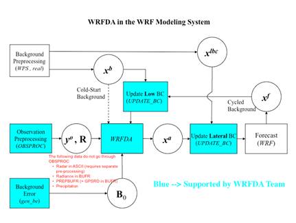
xb first guess, either from a previous WRF forecast or from WPS/REAL output.
xlbc lateral boundary from WPS/REAL output.
xa analysis from the WRFDA data assimilation system.
xf WRF forecast output.
yo observations processed by OBSPROC. (note: PREPBUFR input, radar, radiance, and rainfall data don’t go through OBSPROC)
B0 background error statistics from generic BE data (CV3) or gen_be.
R observational and representative error statistics.
In this chapter, you will learn how to install and run the various components of the WRFDA system. For training purposes, you are supplied with a test case, including the following input data:
· an observation file (which must be processed through OBSPROC),
· a netCDF background file (WPS/REAL output, the first guess of the analysis)
· background error statistics (estimate of errors in the background file).
This tutorial dataset can be downloaded from the WRFDA Users Page (http://www2.mmm.ucar.edu/wrf/users/wrfda/download/testdata.html), and will be described later in more detail. In your own work, however, you will have to create all these input files yourself. See the section Running Observation Preprocessor for creating your observation files. See the section Running gen_be for generating your background error statistics file, if you want to use cv_options=5 or cv_options=6.
Before using your own data, we suggest that you start by running through the WRFDA- related programs using the supplied test case. This serves two purposes: First, you can learn how to run the programs with data we have tested ourselves, and second you can test whether your computer is capable of running the entire modeling system. After you have done the tutorial, you can try running other, more computationally intensive, case studies and experimenting with some of the many namelist variables.
WARNING: It is impossible to test every permutation of computer, compiler, number of processors, case, namelist option, etc. for every WRFDA release. The “namelist” options that are supported are indicated in the “WRFDA/var/README.namelist”, and these are the default options.
Hopefully, our test cases will prepare you for the variety of ways in which you may wish to run your own WRFDA experiments. Please inform us about your experiences.
As a professional courtesy, we request that you include the following references in any publication that uses any component of the community WRFDA system:
Barker, D.M., W. Huang, Y.R. Guo, and Q.N. Xiao., 2004: A
Three-Dimensional (3DVAR) Data Assimilation System For Use With MM5:
Implementation and Initial Results. Mon.
Wea. Rev., 132, 897-914.
Huang, X.Y., Q. Xiao, D.M. Barker, X. Zhang, J. Michalakes,
W. Huang, T. Henderson, J. Bray, Y. Chen, Z. Ma, J. Dudhia, Y. Guo, X. Zhang,
D.J. Won, H.C. Lin, and Y.H. Kuo, 2009: Four-Dimensional Variational Data
Assimilation for WRF: Formulation and Preliminary Results. Mon. Wea. Rev., 137,
299–314.
Running WRFDA requires a Fortran 90 compiler. We have tested the WRFDA on the following platforms: IBM (XLF), SGI Altix (INTEL), PC/Linux (PGI, INTEL, GFORTRAN), and Apple (G95/PGI). Please let us know if this does not meet your requirements, and we will attempt to add other machines to our list of supported architectures, as resources allow. Although we are interested in hearing about your experiences in modifying compiler options, we do not recommend making changes to the configure file used to compile WRFDA.
Installing WRFDA for 3D-Var Run
a. Obtaining
WRFDA Source Code
Users can download the WRFDA
source code from http://www2.mmm.ucar.edu/wrf/users/wrfda/download/get_source.html.
Note: WRF compiles with the –r4 option while WRFDA compiles with –r8. For this reason, WRF and WRFDA cannot reside and be compiled under the same directory.
After the tar file is unzipped (gunzip WRFDAV3.4.TAR.gz) and untarred (tar -xf WRFDAV3.4.TAR), the directory WRFDA should be created. This directory contains the WRFDA source, external libraries, and fixed files. The following is a list of the system components and content for each subdirectory:
|
Directory Name |
Content |
|
var/da |
WRFDA source code |
|
var/run |
Fixed input files required by WRFDA,
such as background error covariance, |
|
var/external |
Library needed by WRFDA, includes CRTM, BUFR, LAPACK, BLAS |
|
var/obsproc |
OBSPROC source code, namelist, and observation error file. |
|
var/gen_be |
Source code of generated background error |
|
var/build |
Builds all .exe files. |
b.
Compile WRFDA and Libraries
Some external libraries (e.g.,
LAPACK, BLAS, and NCEP BUFR) are included in the WRFDA tar file. To compile the
WRFDA code, it is necessary to have installed the netCDF library, which is the
only mandatory library if only conventional observational data in LITTLE_R
format are to be used.
> setenv NETCDF your_netcdf_path
If observational data in the PREPBUFR format are to be used, the NCEP BUFR library must be compiled, and BUFR-related WRFDA code must be generated and compiled after configure/compile. To do this, set the environment variable BUFR before configuring:
>
setenv BUFR 1
If satellite radiance data are to be used, in addition to the NCEP BUFR library, a Radiative Transfer Model (RTM) is required. The current RTM versions that WRFDA uses are CRTM V2.0.2 and RTTOV V10. WRFDA can be compiled with either of these, or both together, but note than only one may be used in each individual run.
Starting with V3.2.1, CRTM V2.0.2
is included in the WRFDA tar file. To have the CRTM library compiled and the
CRTM-related WRFDA code generated and compiled, set the environment variable
CRTM:
>
setenv CRTM 1
If the user wishes to use RTTOV, download and install the RTTOV v10 library before compiling WRFDA. This library can be downloaded from http://research.metoffice.gov.uk/research/interproj/nwpsaf/rtm. After using the RTTOV documentation to compile the library, set the RTTOV environment variable to the path where the lib directory resides. For example, if the library files can be found in /usr/local/rttov10/pgi/lib/librttov10.2.0_*.a, you should set RTTOV as:
> setenv RTTOV /usr/local/rttov10/pgi
Note: Make sure the required libraries were all compiled using the same compiler that will be used to build WRFDA, since the libraries produced by one compiler may not be compatible with code compiled with another.
Assuming all required libraries are available and the WRFDA source code is ready, start to build WRFDA using the following steps:
Set your WRFDA directory as the environment variable WRFDA_DIR. For instance, if your WRFDAV3 directory was unpacked in /usr/local:
>
setenv WRFDA_DIR /usr/local/WRFDAV3
To configure WRFDA, enter the WRFDA directory and run the configure script
> cd
$WRFDA_DIR
> ./configure wrfda
A list of configuration options should appear. Each option combines a compiler type and a parallelism option. Since the configuration script doesn’t check which compilers are actually installed on your system, be sure to select only among the options that are available on your system. The available parallelism options are a single-processor compilation (serial), shared-memory parallel compilation (smpar), distributed-memory parallel compilation (dmpar), and distributed-memory with shared-memory parallel compilation (sm+dm). For example, on a Macintosh computer, the above steps will look similar to the following:
> ./configure wrfda
checking
for perl5... no
checking
for perl... found /usr/bin/perl (perl)
Will use
NETCDF in dir: /users/noname/work/external/g95/netcdf-3.6.1
PHDF5 not
set in environment. Will configure WRF for use without.
$JASPERLIB
or $JASPERINC not found in environment, configuring to build without grib2
I/O...
------------------------------------------------------------------------
Please
select from among the following supported platforms.
1.
Darwin (MACOS) PGI compiler with pgcc
(serial)
2. Darwin (MACOS) PGI compiler with pgcc (smpar)
3.
Darwin (MACOS) PGI compiler with pgcc
(dmpar)
4.
Darwin (MACOS) PGI compiler with pgcc
(dm+sm)
5.
Darwin (MACOS) intel compiler with icc
(serial)
6.
Darwin (MACOS) intel compiler with icc
(smpar)
7.
Darwin (MACOS) intel compiler with icc
(dmpar)
8.
Darwin (MACOS) intel compiler with icc
(dm+sm)
9.
Darwin (MACOS) intel compiler with cc
(serial)
10.
Darwin (MACOS) intel compiler with cc
(smpar)
11.
Darwin (MACOS) intel compiler with cc
(dmpar)
12.
Darwin (MACOS) intel compiler with cc
(dm+sm)
13.
Darwin (MACOS) g95 with gcc
(serial)
14.
Darwin (MACOS) g95 with gcc
(dmpar)
15.
Darwin (MACOS) xlf (serial)
16.
Darwin (MACOS) xlf (dmpar)
Enter
selection [1-10] : 13
------------------------------------------------------------------------
Compile
for nesting? (0=no nesting, 1=basic, 2=preset moves, 3=vortex following)
[default 0]:
Configuration
successful. To build the model type compile .
……
After running the configuration script and choosing a compilation option, a configure.wrf file will be created. Because of the variety of ways that a computer can be configured, if the WRFDA build ultimately fails, there is a chance that minor modifications to the configure.wrf file may be needed.
Hint: It is helpful to start with something simple, such as the serial build. If it is successful, move on to build dmpar code. Remember to type ‘clean –a’ between each build.
To compile the code, type
>
./compile all_wrfvar >&! compile.out
Successful compilation will produce 43 executables: 42 of which are in the var/build directory and linked in the var/da directory, with the 43rd, obsproc.exe, in the var/obsproc/src directory. You can list these executables by issuing the command:
>ls -l
var/build/*exe var/obsproc/src/obsproc.exe
-rwxr-xr-x
1 users 457145 Mar 19 12:18
var/build/da_advance_time.exe
-rwxr-xr-x
1 users 664481 Mar 19 12:18
var/build/da_bias_airmass.exe
-rwxr-xr-x
1 users 503364 Mar 19 12:18 var/build/da_bias_scan.exe
-rwxr-xr-x
1 users 472964 Mar 19 12:18
var/build/da_bias_sele.exe
-rwxr-xr-x
1 users 483459 Mar 19 12:18
var/build/da_bias_verif.exe
-rwxr-xr-x
1 users 109773 Mar 19 12:18
var/build/da_rad_diags.exe
-rwxr-xr-x
1 users 544457 Mar 19 12:18
var/build/da_tune_obs_desroziers.exe
-rwxr-xr-x
1 users 729502 Mar 19 12:18 var/build/da_tune_obs_hollingsworth1.exe
-rwxr-xr-x
1 users 684831 Mar 19 12:18
var/build/da_tune_obs_hollingsworth2.exe
-rwxr-xr-x
1 users 161834 Mar 19 12:18 var/build/da_update_bc_ad.exe
-rwxr-xr-x
1 users 190117 Mar 19 12:18
var/build/da_update_bc.exe
-rwxr-xr-x
1 users 263431 Mar 19 12:18
var/build/da_verif_grid.exe
-rwxr-xr-x
1 users 119380 Mar 19 12:27
var/build/da_verif_obs.exe
-rwxr-xr-x
1 users 12224600 Mar 19 12:30 var/build/da_wrfvar.exe
-rwxr-xr-x
1 users 784425 Mar 19 12:18
var/build/gen_be_cov2d3d_contrib.exe
-rwxr-xr-x
1 users 779660 Mar 19 12:18
var/build/gen_be_cov2d.exe
-rwxr-xr-x
1 users 785577 Mar 19 12:18
var/build/gen_be_cov3d2d_contrib.exe
-rwxr-xr-x
1 users 783375 Mar 19 12:18
var/build/gen_be_cov3d3d_bin3d_contrib.exe
-rwxr-xr-x
1 users 786698 Mar 19 12:18
var/build/gen_be_cov3d3d_contrib.exe
-rwxr-xr-x
1 users 775564 Mar 19 12:18
var/build/gen_be_cov3d.exe
-rwxr-xr-x
1 users 771468 Mar 19 12:18
var/build/gen_be_diags.exe
-rwxr-xr-x
1 users 785285 Mar 19 12:18
var/build/gen_be_diags_read.exe
-rwxr-xr-x
1 users 781914 Mar 19 12:18
var/build/gen_be_ensmean.exe
-rwxr-xr-x
1 users 792143 Mar 19 12:18
var/build/gen_be_ensrf.exe
-rwxr-xr-x
1 users 820618 Mar 19 12:27
var/build/gen_be_ep1.exe
-rwxr-xr-x
1 users 813823 Mar 19 12:27
var/build/gen_be_ep2.exe
-rwxr-xr-x
1 users 818134 Mar 19 12:27
var/build/gen_be_etkf.exe
-rwxr-xr-x
1 users 783755 Mar 19 12:18
var/build/gen_be_hist.exe
-rwxr-xr-x
1 users 843676 Mar 19 12:27
var/build/gen_be_stage0_gsi.exe
-rwxr-xr-x
1 users 830544 Mar 19 12:27
var/build/gen_be_stage0_wrf.exe
-rwxr-xr-x
1 users 808339 Mar 19 12:27
var/build/gen_be_stage1_1dvar.exe
-rwxr-xr-x
1 users 796045 Mar 19 12:27
var/build/gen_be_stage1.exe
-rwxr-xr-x
1 users 808574 Mar 19 12:27
var/build/gen_be_stage1_gsi.exe
-rwxr-xr-x
1 users 940428 Mar 19 12:27
var/build/gen_be_stage2_1dvar.exe
-rwxr-xr-x
1 users 783758 Mar 19 12:27
var/build/gen_be_stage2a.exe
-rwxr-xr-x
1 users 791949 Mar 19 12:27
var/build/gen_be_stage2.exe
-rwxr-xr-x
1 users 573097 Mar 19 12:18
var/build/gen_be_stage2_gsi.exe
-rwxr-xr-x
1 users 791949 Mar 19 12:27
var/build/gen_be_stage3.exe
-rwxr-xr-x
1 users 775572 Mar 19 12:27
var/build/gen_be_stage4_global.exe
-rwxr-xr-x
1 users 796971 Mar 19 12:18
var/build/gen_be_stage4_regional.exe
-rwxr-xr-x
1 users 776963 Mar 19 12:27
var/build/gen_be_vertloc.exe
-rwxr-xr-x
1 users 849562 Mar 19 12:27
var/build/gen_mbe_stage2.exe
-rwxr-xr-x
1 users 880049 Mar 19 12:30
var/obsproc/src/obsproc.exe
The main executable for running WRFDA is da_wrfvar.exe. Make sure it has been created after the compilation: it is possible that all other utilities may get successfully compiled, while the main da_wrfvar.exe fails. If this occurs, please check the compilation log file carefully for any errors.
The basic gen_be utility for the regional model consists of gen_be_stage0_wrf.exe, gen_be_stage1.exe, gen_be_stage2.exe, gen_be_stage2a.exe, gen_be_stage3.exe, gen_be_stage4_regional.exe, and gen_be_diags.exe.
da_updated_bc.exe is used for updating the WRF lower and lateral boundary conditions before and after a new WRFDA analysis is generated.
da_advance_time.exe is a very handy and useful tool for date/time manipulation. Type $WRFDA_DIR/var/build/da_advance_time.exe to see its usage instruction.
obsproc.exe is the executable
for preparing conventional data for WRFDA.
If you specified that BUFR or CRTM libraries were needed, check $WRFDA_DIR/var/external/bufr and $WRFDA_DIR/var/external/crtm to check if the libbufr.a and libcrtm.a were generated.
c.
Clean
Compilation
To remove all object files and executables, type:
clean
To remove all build files, including configure.wrfda, type:
clean -a
The clean –a command is recommended if compilation fails or the configuration file is changed.
Installing WRFPLUS and WRFDA for 4D-Var Run
If you intend to run WRF 4D-Var, it is necessary to have WRFPLUS installed. WRFPLUS contains the adjoint and tangent linear models based on a simplified WRF model, which only includes a few simplified physics packages, such as surface drag, large scale condensation and precipitation, cumulus precipitation. As of V3.4, WRF 4D-Var can be compiled to be run in parallel.
To install WRFPLUS V3.4:
- Get the WRFPLUS zipped tar file from http://www2.mmm.ucar.edu/wrf/users/wrfda/download/wrfplus.html
- Unzip and untar the file for WRFPLUS, then run the configure script
> gunzip
WRFPLUSV3.4.TAR.gz
> tar -xf
WRFPLUSV3.4.TAR
> cd
WRFPLUSV3
> ./configure
wrfplus
As with 3D-Var, “serial” means single-processor, and “dmpar” means Distributed Memory Parallel (MPI)
- Compile WRFPLUS
> ./compile
em_real
> ls -ls
main/*.exe
You should see the following files:
-rwxr-xr-x
1 user users 23179920 Apr 3 15:22
main/ndown.exe
-rwxr-xr-x
1 user users 22947466 Apr 3 15:22
main/nup.exe
-rwxr-xr-x
1 user users 23113961 Apr 3 15:22
main/real.exe
-rwxr-xr-x
1 user users 22991725 Apr 3 15:22
main/tc.exe
-rwxr-xr-x
1 user users 32785447 Apr 3 15:20
main/wrf.exe
Finally, set the environment variable WRFPLUS_DIR to the appropriate directory:
>setenv
WRFPLUS_DIR ${your_source_code_dir}/WRFPLUSV3
To install WRFDA for the 4D-Var run:
- If you intend to use observational data in the PREPBUFR format, or if you intend to assimilate satellite radiance data, you need to set environment variables for BUFR, CRTM, and/or RTTOV. See the previous 3D-Var section for instructions.
>./configure 4dvar >& compile.out
Note: As of V3.4, WRFDA 4D-Var may be compiled to run in parallel mode.
>./compile
all_wrfvar
>ls -ls var/build/*.exe var/obsproc/*.exe
You should see the same 43 executables as
are listed in the above 3D-Var section, including da_wrfvar.exe
Running Observation Preprocessor (OBSPROC)
The OBSPROC program reads observations in LITTLE_R format (a legendary ASCII format, in use since the MM5 era). The LITTLE_R format is also used in the OBSGRID program. Please refer to the documentation in Chapter 7 of this User’s Guide for the LITTLE_R format description. For your applications, besides those observations provided for the tutorial case, you will have to prepare your own observation files. Please see http://www2.mmm.ucar.edu/wrf/users/wrfda/download/free_data.html for the sources of some freely-available observations. Because the raw observation data files have many possible formats, such as ASCII, BUFR, PREPBUFR, MADIS, and HDF, the free data site also contains instructions for converting the observations to LITTLE_R format. To make the WRFDA system as general as possible, the LITTLE_R format was adopted as an intermediate observation data format for the WRFDA system, however, the conversion of the user-specific source data to the LITTLE_R format observation data file is the user’s task. A more complete description of the LITTLE_R format and conventional observation data sources for WRFDA can be found by reading the tutorial found at http://www2.mmm.ucar.edu/wrf/users/wrfda/Tutorials/2010_Aug/tutorial_presentation_summer_2010.html.
The purposes of OBSPROC are to:
· Remove observations outside the specified temporal and spatial domains
· Re-order and merge duplicate (in time and location) data reports
· Retrieve pressure or height based on observed information using the hydrostatic assumption
· Check multi-level observations for vertical consistency and super adiabats
· Assign observational errors based on a pre-specified error file
· Write out the observation file to be used by WRFDA in ASCII or BUFR format
The OBSPROC program (obsproc.exe) should be found under the directory $WRFDA_DIR/var/obsproc/src if “compile all_wrfvar” completed successfully.
a. Prepare observational data for 3D-Var
As an example, to prepare the observation file at the analysis time (0h for 3D-Var), all the observations in the range ±1h will be processed, which means that the observations between 23h and 1h are treated as the observations at 0h. This is illustrated in the following figure:
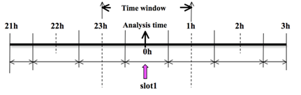
Before running obsproc.exe, create the required namelist file namelist.obsproc (see $WRFDA_DIR/var/obsproc/README.namelist, or the section Description of Namelist Variables for details.
For your reference, the example file namelist_obsproc.3dvar.wrfvar-tut has been provided in the var/obsproc directory. Thus, proceed as follows.
> cd
$WRFDA_DIR/var/obsproc
> cp namelist.obsproc.3dvar.wrfvar-tut namelist.obsproc
Next, edit the namelist file, namelist.obsproc, to accommodate your experiments. You will likely only need to change variables listed under records 1, 2, 6, 7, and 8. See the section Description of Namelist Variables for details; you should pay special attention to NESTIX and NESTJX.
If you are running the tutorial case, you should copy or link the sample observation file (ob/2008020512/obs.2008020512) to the obsproc directory. Alternatively, you can edit the namelist variable obs_gts_filename to point to the observation file’s full path.
To run OBSPROC, type
> obsproc.exe >&! obsproc.out
Once obsproc.exe has completed successfully, you will see an observation data file, with the name formatted obs_gts_YYYY-MM-DD_HH:NN:SS.3DVAR, in the obsproc directory. For the tutorial case, this will be obs_gts_2008-02-05_12:00:00.3DVAR. This is the input observation file to WRFDA. It is an ASCII file that contains a header section (listed below) followed by observations. The meanings and format of observations in the file are described in the last six lines of the header section.
TOTAL
= 9066, MISS. =-888888.,
SYNOP
= 757, METAR = 2416, SHIP
= 145, BUOY =
250, BOGUS = 0, TEMP =
86,
AMDAR
= 19, AIREP = 205, TAMDAR= 0, PILOT = 85, SATEM = 106, SATOB = 2556,
GPSPW
= 187, GPSZD = 0, GPSRF = 3, GPSEP = 0, SSMT1 = 0, SSMT2 = 0,
TOVS =
0, QSCAT = 2190, PROFL = 61, AIRSR = 0, OTHER = 0,
PHIC =
40.00, XLONC = -95.00, TRUE1 =
30.00, TRUE2 = 60.00, XIM11
= 1.00, XJM11 = 1.00,
base_temp=
290.00, base_lapse= 50.00, PTOP =
1000., base_pres=100000., base_tropo_pres= 20000., base_strat_temp= 215.,
IXC =
60, JXC = 90, IPROJ = 1, IDD
= 1, MAXNES= 1,
NESTIX= 60,
NESTJX= 90,
NUMC =
1,
DIS =
60.00,
NESTI
= 1,
NESTJ
= 1,
INFO = PLATFORM, DATE, NAME, LEVELS, LATITUDE,
LONGITUDE, ELEVATION, ID.
SRFC = SLP, PW (DATA,QC,ERROR).
EACH = PRES, SPEED, DIR, HEIGHT, TEMP, DEW PT,
HUMID (DATA,QC,ERROR)*LEVELS.
INFO_FMT
= (A12,1X,A19,1X,A40,1X,I6,3(F12.3,11X),6X,A40)
SRFC_FMT
= (F12.3,I4,F7.2,F12.3,I4,F7.3)
EACH_FMT
= (3(F12.3,I4,F7.2),11X,3(F12.3,I4,F7.2),11X,3(F12.3,I4,F7.2))
#------------------------------------------------------------------------------#
……
observations ………
Before running WRFDA, you may find it useful to learn more about various types of data that will be processed to WRFDA (e.g., their geographical distribution). This file is in ASCII format and so you can easily view it. For a graphical view of the file's content, use the MAP_plot utility to see the data distribution for each type of observation. To use this utility, proceed to the MAP_plot directory, then compile by typing “make”.
If the build fails, it is likely
due to an improper configuration file. By viewing the contents of the MAP_plot
directory, you will see we have prepared some
configure.user.ibm/OS
files (where OS is the type of operating system) for some platforms. When “make” is typed, the Makefile uses one of them to determine the
compiler and compiler option. Modify the Makefile
and configure.user.xxx
to accommodate the complier on your platform, then type “make” to attempt the compilation again. Successful
compilation will produce Map.exe.
The following instructions are for the tutorial case, but can easily be
configured for your own data by changing the appropriate dates and file names.
Note: The successful
compilation of Map.exe requires pre-installed NCARG Graphics libraries
under $(NCARG_ROOT)/lib.
Modify the script Map.csh to set the time window and full path of the input observation file (obs_gts_2008-02-05_12:00:00.3DVAR). You will need to set the following strings in this script as follows:
Map_plot
= $WRFDA_DIR/var/obsproc/MAP_plot
TIME_WINDOW_MIN
= ‘2008020511’
TIME_ANALYSIS = ‘2008020512’
TIME_WINDOW_MAX
= ‘2008020513’
OBSDATA
= ../obs_gts_2008-02-05_12:00:00.3DVAR
Next, type Map.csh
to run the script
When the job has completed, you
will have a gmeta file, gmeta.2008020512. This contains plots of data distribution for each
type of observation contained in the OBS data file: obs_gts_2008-02-05_12:00:00.3DVAR. To view
this, type
> idt
gmeta.2008020512
It will display a panel-by-panel geographical distribution of various types of data. The following graphic shows the geographic distribution of sonde observations for this case.
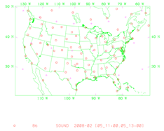
An alternative way to plot the observations is to use an NCL script (for more information on NCL, the NCAR Command Language, see http://www.ncl.ucar.edu/). In the WRFDA Tools package (can be downloaded at http://www2.mmm.ucar.edu/wrf/users/wrfda/download/tools.html), this script is located at $TOOLS_DIR/var/graphics/ncl/plot_ob_ascii_loc.ncl. With this method, however, you need to provide the first guess file to the NCL script, and have NCL installed in your system.
b. Prepare observational data for 4D-Var
To prepare the observation file, for example, at the analysis time 0h for 4D-Var, all observations from 0h to 6h will be processed and grouped in 7 sub-windows (slot1 through slot7) as illustrated in the following figure:
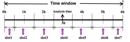
NOTE: The “Analysis time” in the above figure is not the actual analysis time (0h). It indicates the time_analysis setting in the namelist file and is set to three hours later than the actual analysis time. The actual analysis time is still 0h.
An example file (namelist_obsproc.4dvar.wrfvar-tut) has already been provided in the var/obsproc directory. Thus, proceed as follows:
> cd
$WRFDA_DIR/var/obsproc
> cp namelist.obsproc.4dvar.wrfvar-tut namelist.obsproc
In the namelist file, you need to change the following variables to accommodate your experiments. In this tutorial case, the actual analysis time is 2008-02-05_12:00:00, but in the namelist, the time_analysis should be set to 3 hours later. The different values of time_analysis, num_slots_past, and time_slots_ahead contribute to the actual times analyzed. For example, if you set time_analysis = 2008-02-05_16:00:00, and set the num_slots_past = 4 and time_slots_ahead=2, the final results will be the same as before.
Edit all the domain settings according to your own experiment. You should pay special attention to NESTIX and NESTJX, which is described in the section Description of Namelist Variables for details.
To run OBSPROC, type
>
obsproc.exe >&! obsproc.out
Once obsproc.exe has completed successfully, you
will see 7 observation data files, which for the tutorial case are named
obs_gts_2008-02-05_12:00:00.4DVAR
obs_gts_2008-02-05_13:00:00.4DVAR
obs_gts_2008-02-05_14:00:00.4DVAR
obs_gts_2008-02-05_15:00:00.4DVAR
obs_gts_2008-02-05_16:00:00.4DVAR
obs_gts_2008-02-05_17:00:00.4DVAR
obs_gts_2008-02-05_18:00:00.4DVAR
They are the input observation files to WRF 4D-Var. As with 3D-Var, you can use MAP_Plot to view the geographic distribution of different observations at different time slots.
Running WRFDA
a. Download Test Data
The WRFDA system requires three input files to run:
a) WRF first guess and boundary input files output from either WPS/real (cold-start) or WRF forecast (warm-start)
b) Observations (in ASCII format, PREPBUFR or BUFR for radiance)
c) A background error statistics file (containing background error covariance)
The following table summarizes the above info:
|
Input Data |
Format |
Created By |
|
First Guess |
NETCDF |
WRF Preprocessing System (WPS) and real.exe or WRF |
|
Observations |
ASCII (PREPBUFR also possible) |
Observation Preprocessor (OBSPROC) |
|
Background Error Statistics |
Binary |
or generic CV3 |
In the test case, you will store data in a directory defined by the environment variable $DAT_DIR. This directory can be in any location, and it should have read access. Type
> setenv DAT_DIR your_choice_of_dat_dir
Here, your_choice_of_dat_dir is the directory where the WRFDA input data is stored. If it does not exist, create this directory by typing
> mkdir $DAT_DIR
Download the test data for a the tutorial case, valid at 12 UTC 5th February 2008, from http://www2.mmm.ucar.edu/wrf/users/wrfda/download/testdata.html
Once you have downloaded the WRFDAV3.4-testdata.tar.gz file to $DAT_DIR, extract it by typing
> gunzip WRFDAV3.4-testdata.tar.gz
> tar -xvf WRFDAV3.4-testdata.tar
Now you should find the following
four files under “$DAT_DIR”
ob/2008020512/ob.2008020512 #
Observation data in “little_r” format
rc/2008020512/wrfinput_d01
# First guess file
rc/2008020512/wrfbdy_d01
# lateral boundary file
be/be.dat
#
Background error file
......
At this point you should have
three of the input files (first guess, observations from OBSPROC, and
background error statistics files in the directory $DAT_DIR) required to run WRFDA, and have successfully
downloaded and compiled the WRFDA code. If this is correct, you are ready to
learn how to run WRFDA.
b. Run the Case—3D-Var
The data for the tutorial case is valid at 12 UTC 5 February 2008. The first guess comes from the NCEP FNL (Final) Operational Global Analysis data, passed through the WRF-WPS and real programs.
To run WRF 3D-Var, first create and enter into a working directory (for example, $WRFDA_DIR/workdir), and set the environment variable WORK_DIR to this directory (e.g., setenv WORK_DIR $WRFDA_DIR/workdir). Then follow the steps below:
> cd $WORK_DIR
> cp
$WRFDA_DIR/var/test/tutorial/namelist.input .
> ln -sf $WRFDA_DIR/run/LANDUSE.TBL
.
> ln -sf
$DAT_DIR/rc/2008020512/wrfinput_d01 ./fg
> ln -sf $WRFDA_DIR/var/obsproc/obs_gts_2008-02-05_12:00:00.3DVAR
./ob.ascii (note the different name!)
> ln -sf $DAT_DIR/be/be.dat .
> ln -sf $WRFDA_DIR/var/da/da_wrfvar.exe
.
Now edit the file namelist.input, which is a very basic namelist for the tutorial test case, and is shown below.
&wrfvar1
var4d=false,
print_detail_grad=false,
/
&wrfvar2
/
&wrfvar3
ob_format=2,
/
&wrfvar4
/
&wrfvar5
/
&wrfvar6
max_ext_its=1,
ntmax=50,
orthonorm_gradient=true,
/
&wrfvar7
cv_options=5,
/
&wrfvar8
/
&wrfvar9
/
&wrfvar10
test_transforms=false,
test_gradient=false,
/
&wrfvar11
/
&wrfvar12
/
&wrfvar13
/
&wrfvar14
/
&wrfvar15
/
&wrfvar16
/
&wrfvar17
/
&wrfvar18
analysis_date="2008-02-05_12:00:00.0000",
/
&wrfvar19
/
&wrfvar20
/
&wrfvar21
time_window_min="2008-02-05_11:00:00.0000",
/
&wrfvar22
time_window_max="2008-02-05_13:00:00.0000",
/
&wrfvar23
/
&time_control
start_year=2008,
start_month=02,
start_day=05,
start_hour=12,
end_year=2008,
end_month=02,
end_day=05,
end_hour=12,
/
&fdda
/
&domains
e_we=90,
e_sn=60,
e_vert=41,
dx=60000,
dy=60000,
/
&dfi_control
/
&tc
/
&physics
mp_physics=3,
ra_lw_physics=1,
ra_sw_physics=1,
radt=60,
sf_sfclay_physics=1,
sf_surface_physics=1,
bl_pbl_physics=1,
cu_physics=1,
cudt=5,
num_soil_layers=5,
mp_zero_out=2,
co2tf=0,
/
&scm
/
&dynamics
/
&bdy_control
/
&grib2
/
&fire
/
&namelist_quilt
/
&perturbation
/
No edits should be needed if you are running the tutorial case without radiance data. If you plan to use the PREPBUFR format data, change the ob_format=1 in &wrfvar3 in namelist.input and link the data as ob.bufr,
> ln -fs
$DAT_DIR/ob/2008020512/gds1.t12.prepbufr.nr
ob.bufr
Please note: Although WRFDA does not include any physics packages listed in &physics, users still have to keep the namelist options in &physics the same as which in your firstguess (use “ncdump –h fg” to get the physics options the firstguess uses), as the WRFDA I/O utility decides which 4D variables will be output based on the physics options.
Once you have changed any other necessary namelist variables, run WRFDA 3D-Var:
>
da_wrfvar.exe >&! wrfda.log
The file wrfda.log (or rsl.out.0000, if run in distributed-memory mode) contains important WRFDA runtime log information. Always check the log after a WRFDA run:
*** VARIATIONAL ANALYSIS ***
DYNAMICS OPTION: Eulerian Mass Coordinate
alloc_space_field: domain 1, 606309816 bytes allocat
ed
WRF TILE
1 IS 1 IE 89 JS
1 JE 59
WRF NUMBER OF TILES = 1
Set up
observations (ob)
Using
ASCII format observation input
scan obs ascii
end scan obs ascii
Observation
summary
ob time
1
sound 86 global, 86 local
synop 757 global, 750 local
pilot 85 global, 85 local
satem 106 global, 105 local
geoamv 2556 global, 2499 local
polaramv 0 global, 0 local
airep 224 global,
221 local
gpspw 187 global, 187 local
gpsrf 3 global, 3 local
metar 2416 global, 2408 local
ships 145 global, 140 local
ssmi_rv
0 global, 0 local
ssmi_tb 0 global, 0 local
ssmt1 0 global, 0 local
ssmt2 0 global, 0 local
qscat 2190 global, 2126 local
profiler 61 global, 61 local
buoy 247 global, 247 local
bogus 0 global, 0 local
pseudo 0 global, 0 local
radar 0 global, 0 local
radiance 0 global, 0 local
airs retrieval 0 global, 0 local
sonde_sfc 86 global, 86 local
mtgirs 0 global, 0 local
tamdar 0 global, 0
local
Set up
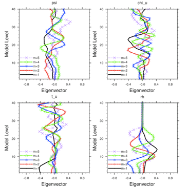
background errors for regional application for cv_options = 5
Using the averaged regression coefficients
for unbalanced part
WRF-Var dry control variables are:psi,
chi_u, t_u and ps_u
Humidity control variable is rh
Vertical
truncation for psi = 15(
99.00%)
Vertical
truncation for chi_u = 20(
99.00%)
Vertical
truncation for t_u = 29(
99.00%)
Vertical
truncation for rh = 22(
99.00%)
Scaling: var, len, ds: 0.100000E+01 0.100000E+01 0.600000E+05
Scaling: var, len, ds: 0.100000E+01 0.100000E+01 0.600000E+05
Scaling: var, len, ds: 0.100000E+01 0.100000E+01 0.600000E+05
Scaling: var, len, ds: 0.100000E+01 0.100000E+01 0.600000E+05
Scaling: var, len, ds: 0.100000E+01 0.100000E+01 0.600000E+05
Calculate
innovation vector(iv)
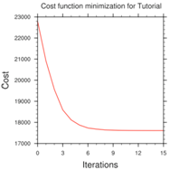
Minimize
cost function using CG method
Starting
outer iteration : 1
Starting
cost function: 2.53214888D+04,
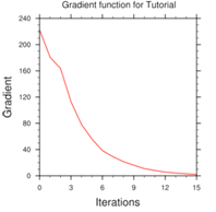
Gradient= 2.90675545D+02
For this
outer iteration gradient target is:
2.90675545D+00
----------------------------------------------------------
Iter Cost Function Gradient Step
1
2.32498037D+04
2.55571188D+02 4.90384516D-02
2
2.14988144D+04
2.22354203D+02 5.36154186D-02
3
2.01389088D+04
1.62537907D+02 5.50108123D-02
4
1.93433827D+04
1.26984567D+02 6.02247687D-02
5
1.88877194D+04
9.84565874D+01 5.65160951D-02
6
1.86297777D+04
7.49071361D+01 5.32184146D-02
7
1.84886755D+04
5.41516421D+01 5.02941363D-02
8
1.84118462D+04
4.68329312D+01 5.24003071D-02
9
1.83485166D+04
3.53595537D+01 5.77476335D-02
10
1.83191278D+04
2.64947070D+01 4.70109040D-02
11
1.82984221D+04
2.06996271D+01 5.89930206D-02
12
1.82875693D+04
1.56426527D+01 5.06578447D-02
13
1.82807224D+04
1.15892153D+01 5.59631997D-02
14
1.82773339D+04
8.74778514D+00 5.04582959D-02
15
1.82751663D+04
7.22150257D+00 5.66521675D-02
16
1.82736284D+04
4.81374868D+00 5.89786400D-02
17
1.82728636D+04
3.82286871D+00 6.60104384D-02
18
1.82724306D+04
3.16737517D+00 5.92526480D-02
19
1.82721735D+04
2.23392283D+00 5.12604438D-02
----------------------------------------------------------
Inner
iteration stopped after 19 iterations
Final: 19 iter, J= 1.98187399D+04, g= 2.23392283D+00
----------------------------------------------------------
Diagnostics
Final cost function J =
19818.74
Total number of obs. =
39800
Final value of J = 19818.73988
Final value of Jo =
16859.85861
Final value of Jb = 2958.88127
Final value of Jc = 0.00000
Final value of Je = 0.00000
Final value of Jp = 0.00000
Final value of Jl = 0.00000
Final J / total num_obs =
0.49796
Jb factor used(1) = 1.00000 1.00000 1.00000 1.00000 1.00000
1.00000 1.00000 1.00000 1.00000 1.00000
Jb factor used(2) = 1.00000 1.00000 1.00000 1.00000 1.00000
1.00000 1.00000 1.00000 1.00000 1.00000
Jb factor used(3) = 1.00000 1.00000 1.00000 1.00000 1.00000
1.00000 1.00000 1.00000 1.00000 1.00000
Jb factor used(4) = 1.00000 1.00000 1.00000 1.00000 1.00000
1.00000 1.00000 1.00000 1.00000 1.00000
Jb factor used(5) = 1.00000 1.00000 1.00000 1.00000 1.00000
1.00000 1.00000 1.00000 1.00000 1.00000
Jb factor used = 1.00000
Je factor used = 1.00000
VarBC factor used = 1.00000
*** WRF-Var completed successfully ***
The file namelist.output (which contains the complete namelist settings) will be generated after a successful run of da_wrfvar.exe. The settings appearing in namelist.output, but not specified in your namelist.input, are the default values from $WRFDA_DIR/Registry/Registry.wrfvar.
After successful completion, wrfvar_output (the WRFDA analysis file, i.e. the new initial condition for WRF) should appear in the working directory along with a number of diagnostic files. Various text diagnostics output files will be explained in the next section (WRFDA Diagnostics).
To understand the role of various important WRFDA options, try re-running WRFDA by changing different namelist options. For example, try making the WRFDA convergence criterion more stringent. This is achieved by reducing the value of “EPS” to e.g. 0.0001 by adding "EPS=0.0001" in the namelist.input record &wrfvar6. See the section (WRFDA additional exercises) for more namelist options.
c. Run the Case—4D-Var
To run WRF 4D-Var, first create and enter a working directory, such as $WRFDA_DIR/workdir. Set the WORK_DIR environment variable (e.g. setenv WORK_DIR $WRFDA_DIR/workdir)
For the tutorial case, the analysis date is 2008020512 and the test data directories are:
>
setenv DAT_DIR {directory where data is stored}
> ls
–lr $DAT_DIR
ob/2008020512
ob/2008020513
ob/2008020514
ob/2008020515
ob/2008020516
ob/2008020517
ob/2008020518
rc/2008020512
be
Note: WRFDA 4D-Var is able to assimilate conventional observational data, satellite radiance BUFR data, radar data, and precipitation data. The input data format can be PREPBUFR format data or observation data, processed by OBSPROC.
Now follow the steps below:
1) Link the executables.
> cd
$WORK_DIR
> ln
-fs $WRFDA_DIR/var/da/da_wrfvar.exe .
2) Link the observational data, first guess, BE and LANDUSE.TBL, etc.
> ln
-fs $DAT_DIR/ob/2008020512/ob.ascii+ ob01.ascii
> ln
-fs $DAT_DIR/ob/2008020513/ob.ascii
ob02.ascii
> ln
-fs $DAT_DIR/ob/2008020514/ob.ascii
ob03.ascii
> ln
-fs $DAT_DIR/ob/2008020515/ob.ascii
ob04.ascii
> ln
-fs $DAT_DIR/ob/2008020516/ob.ascii
ob05.ascii
> ln
-fs $DAT_DIR/ob/2008020517/ob.ascii
ob06.ascii
> ln
-fs $DAT_DIR/ob/2008020518/ob.ascii- ob07.ascii
> ln
-fs $DAT_DIR/rc/2008020512/wrfinput_d01 .
> ln
-fs $DAT_DIR/rc/2008020512/wrfbdy_d01 .
> ln
-fs wrfinput_d01 fg
> ln
-fs $DAT_DIR/be/be.dat .
> ln
-fs $WRFDA_DIR/run/LANDUSE.TBL .
> ln
-fs $WRFDA_DIR/run/GENPARM.TBL .
> ln
-fs $WRFDA_DIR/run/SOILPARM.TBL .
> ln
-fs $WRFDA_DIR/run/VEGPARM.TBL .
> ln
–fs $WRFDA_DIR/run/RRTM_DATA_DBL RRTM_DATA
3) Copy the sample namelist
> cp $WRFDA_DIR/var/test/4dvar/namelist.input
.
4) Edit necessary namelist variables, link optional files
Starting with V3.4, WRFDA 4D-Var has the capability to consider lateral boundary conditions as control variables as well during minimization. The namelist variable var4d_lbc=true turns on this capability. To enable this option, WRF 4D-Var needs not only the first guess at the beginning of the time window, but also the first guess at the end of the time window.
> ln -fs $DAT_DIR/rc/2008020518/wrfinput_d01 fg02
Please note: For WRFDA beginner, please don’t use this option
before you have a good understanding of the 4D-Var lateral boundary conditions control.
To disable this feature, make sure var4d_lbc in
namelist.input is set to false.
If you use PREPBUFR format data, set ob_format=1 in &wrfvar3 in namelist.input. Because 12UTC PREPBUFR data only includes the data from 9UTC to 15UTC, for 4D-Var you should include 18UTC PREPBUFR data as well:
> ln
-fs $DAT_DIR/ob/2008020512/gds1.t12.prepbufr.nr
ob01.bufr
> ln
-fs $DAT_DIR/ob/2008020518/gds1.t18.prepbufr.nr
ob02.bufr
Note: NCEP BUFR files downloaded from NCEP’s public ftp server (ftp://ftp.ncep.noaa.gov/pub/data/nccf/com/gfs/prod/gdas.${yyyymmddhh}) are Fortran-blocked on a big-endian machine and can be directly used on big-endian machines (for example, IBM). For most Linux clusters with Intel platforms, users need to download the byte-swapping code ssrc.c (http://www.dtcenter.org/com-GSI/users/support/faqs/index.php). The C code ssrc.c is located in the /utils directory of the GSI distribution. This code will convert a prepbufr file generated on an IBM platform to a prepbufr file that can be read on a Linux or Intel Mac platform. Compile ssrc.c with any c compiler (e.g., gcc -o ssrc.exe ssrc.c). To convert an IBM prepbufr file, take the executable (e.g. ssrc.exe), and run it as follows:
ssrc.exe <Big Endian
prepbufr file> Little Endian prepbufr file
Edit $WORK_DIR/namelist.input to match your experiment settings. The most important namelist variables related to 4D-Var are listed below. Please refer to README.namelist under the $WRFDA_DIR/var directory. Common mistakes users make are in the time information settings. The rules are: analysis_date, time_window_min and start_xxx in &time_control should always be equal to each other; time_window_max and end_xxx should always be equal to each other; and run_hours is the difference between start_xxx and end_xxx, which is the length of the 4D-Var time window.
&wrfvar1
var4d=true,
var4d_lbc=false,
var4d_bin=3600,
……
/
……
&wrfvar18
analysis_date="2008-02-05_12:00:00.0000",
/
……
&wrfvar21
time_window_min="2008-02-05_12:00:00.0000",
/
……
&wrfvar22
time_window_max="2008-02-05_18:00:00.0000",
/
……
&time_control
run_hours=6,
start_year=2008,
start_month=02,
start_day=05,
start_hour=12,
end_year=2008,
end_month=02,
end_day=05,
end_hour=18,
interval_seconds=21600,
debug_level=0,
/
……
5) Run WRF 4D-Var
> cd
$WORK_DIR
>
./da_wrfvar.exe >&! wrfda.log
Please note: If you utilize the lateral boundary conditions option (var4d_lbc=true), in addition to the analysis at the beginning of the time window (wrfvar_output), the analysis at the end of the time window will also be generated as ana02, which will be used in subsequent updating of boundary conditions before the forecast.
Radiance Data Assimilation in WRFDA
This section gives a brief description for various aspects
related to radiance assimilation in WRFDA. Each aspect is described mainly from
the viewpoint of usage, rather than more technical and scientific details,
which will appear in a separate technical report and scientific paper. Namelist
parameters controlling different aspects of radiance assimilation will be detailed
in the following sections. It should be noted that this section does not cover
general aspects of the assimilation process with WRFDA; these can be found in
other sections of chapter 6 of this user’s guide, or other WRFDA documentation.
a. Running WRFDA with radiances
In addition to the basic input files (LANDUSE.TBL, fg, ob.ascii, be.dat) mentioned in the “Running
WRFDA” section, the
following additional files are required for radiances: radiance data in NCEP
BUFR format, radiance_info files, VARBC.in,
and RTM (CRTM or RTTOV) coefficient files.
Edit namelist.input (Pay special attention to &wrfvar4, &wrfvar14, &wrfvar21, and
&wrfvar22 for radiance-related options. A
very basic namelist.input for running the radiance test case is provided in WRFDA/var/test/radiance/namelist.input)
> ln
-sf $DAT_DIR/gdas1.t00z.1bamua.tm00.bufr_d
./amsua.bufr
> ln
-sf $DAT_DIR/gdas1.t00z.1bamub.tm00.bufr_d
./amsub.bufr
> ln
-sf $WRFDA_DIR/var/run/radiance_info
./radiance_info # (radiance_info
is a directory)
> ln
-sf $WRFDA_DIR/var/run/VARBC.in
./VARBC.in
(CRTM
only) > ln -sf
WRFDA/var/run/crtm_coeffs ./crtm_coeffs
#(crtm_coeffs is a directory)
(RTTOV
only) > ln -sf your_RTTOV_path/rtcoef_rttov10/rttov7pred51L ./rttov_coeffs #
(rttov_coeffs is a directory)
See the following sections for more details on each aspect
of radiance assimilation.
b. Radiance Data Ingest
Currently, the ingest interface for NCEP BUFR radiance data
is implemented in WRFDA. The radiance data are available through NCEP’s public
ftp server (ftp://ftp.ncep.noaa.gov/pub/data/nccf/com/gfs/prod/gdas.${yyyymmddhh})
in near real-time (with a 6-hour delay) and can meet requirements for both
research purposes and some real-time applications.
As of Version 3.4, WRFDA can read data from the NOAA ATOVS
instruments (HIRS, AMSU-A, AMSU-B and MHS), the EOS Aqua instruments (AIRS,
AMSU-A) and DMSP instruments (SSMIS). Note that NCEP radiance BUFR files are
separated by instrument names (i.e., one file for each type of instrument), and
each file contains global radiance (generally converted to brightness
temperature) within a 6-hour assimilation window, from multi-platforms. For
running WRFDA, users need to rename NCEP corresponding BUFR files (table 1) to hirs3.bufr (including HIRS data from NOAA-15/16/17), hirs4.bufr (including HIRS data from NOAA-18/19, METOP-2), amsua.bufr (including AMSU-A data from NOAA-15/16/18/19, METOP-2), amsub.bufr (including AMSU-B data from NOAA-15/16/17), mhs.bufr (including MHS data from NOAA-18/19 and METOP-2), airs.bufr (including AIRS and AMSU-A data from EOS-AQUA) and ssmis.bufr (SSMIS data from DMSP-16, AFWA provided) for WRFDA
filename convention. Note that the airs.bufr file
contains not only AIRS data but also AMSU-A, which is collocated with AIRS
pixels (1 AMSU-A pixel collocated with 9 AIRS pixels). Users must place these
files in the working directory where the WRFDA executable is run. It should
also be mentioned that WRFDA reads these BUFR radiance files directly without
the use of any separate pre-processing program. All processing of radiance
data, such as quality control, thinning, bias correction, etc., is carried out
within WRFDA. This is different from conventional observation assimilation,
which requires a pre-processing package (OBSPROC) to generate WRFDA readable
ASCII files. For reading the radiance BUFR files, WRFDA must be compiled with
the NCEP BUFR library (see http://www.nco.ncep.noaa.gov/sib/decoders/BUFRLIB/).
Table 1: NCEP and WRFDA radiance BUFR file naming convention
|
NCEP BUFR file names |
WRFDA naming convention |
|
gdas1.t00z.1bamua.tm00.bufr_d |
amsua.bufr |
|
gdas1.t00z.1bamub.tm00.bufr_d |
amsub.bufr |
|
gdas1.t00z.1bhrs3.tm00.bufr_d |
hirs3.bufr |
|
gdas1.t00z.1bhrs4.tm00.bufr_d |
hirs4.bufr |
|
gdas1.t00z.1bmhs.tm00.bufr_d |
mhs.bufr |
|
gdas1.t00z.airsev.tm00.bufr_d |
airs.bufr |
Namelist parameters are used to control the reading of
corresponding BUFR files into WRFDA. For instance, USE_AMSUAOBS, USE_AMSUBOBS, USE_HIRS3OBS, USE_HIRS4OBS, USE_MHSOBS, USE_AIRSOBS, USE_EOS_AMSUAOBS and USE_SSMISOBS control whether or not
the respective file is read. These are logical parameters that are assigned to
.FALSE. by default; therefore they must be set to .TRUE. to read the respective observation file. Also note that
these parameters only control whether the data is read, not whether the data
included in the files is to be assimilated. This is controlled by other
namelist parameters explained in the next section.
NCEP BUFR files downloaded from NCEP’s public ftp server (ftp://ftp.ncep.noaa.gov/pub/data/nccf/com/gfs/prod/gdas.${yyyymmddhh})
are Fortran-blocked on a big-endian machine and can be directly used on
big-endian machines (for example, IBM). For most Linux clusters with Intel
platforms, users need to download the byte-swapping code ssrc.c (http://www.dtcenter.org/com-GSI/users/support/faqs/index.php). The C code ssrc.c is located in the /utils directory of
the GSI distribution, and will convert a PREPBUFR file generated on an IBM
platform to a PREPBUFR file that can be read on a Linux or Intel Mac platform.
Compile ssrc.c with any c compiler (e.g.,
gcc -o ssrc.exe ssrc.c). To convert an IBM PREPBUFR file, take the executable (e.g.
ssrc.exe),
and run it as follows:
ssrc.exe
< Big Endian prepbufr file> Little Endian prepbufr file
c. Radiative Transfer Model
The core component for direct radiance assimilation is to
incorporate a radiative transfer model (RTM) into the WRFDA system as one part
of observation operators. Two widely used RTMs in the NWP community, RTTOV
(developed by ECMWF and UKMET in Europe), and CRTM (developed by the Joint
Center for Satellite Data Assimilation (JCSDA) in US), are already implemented
in the WRFDA system with a flexible and consistent user interface. WRFDA is
designed to be able to compile with any combination of the two RTM libraries,
or without RTM libraries (for those not interested in radiance assimilation),
by the definition of environment variables “CRTM” and “RTTOV” (see the
“Installing WRFDA” section). Note, however, that at runtime the user must select
one of the two or neither, via the namelist parameter RTM_OPTION (1 for RTTOV, the default,
and 2 for CRTM).
Both RTMs can calculate radiances for almost all available
instruments aboard the various satellite platforms in orbit. An important
feature of the WRFDA design is that all data structures related to radiance
assimilation are dynamically allocated during running time, according to a
simple namelist setup. The instruments to be assimilated are controlled at
run-time by four integer namelist parameters: RTMINIT_NSENSOR (the total number
of sensors to be assimilated), RTMINIT_PLATFORM (the platforms IDs array to be assimilated with dimension
RTMINIT_NSENSOR, e.g., 1 for NOAA, 9 for EOS, 10 for METOP and 2 for DMSP), RTMINIT_SATID (satellite IDs array)
and RTMINIT_SENSOR (sensor IDs array, e.g., 0 for HIRS, 3 for AMSU-A, 4 for
AMSU-B, 15 for MHS, 10 for SSMIS, 11 for AIRS). An example configuration for
assimilating 14 of the sensors from 7 satellites is listed here:
RTMINIT_NSENSOR
= 14 # 6 AMSUA; 3 AMSUB; 3 MHS; 1 AIRS; 1 SSMIS
RTMINIT_PLATFORM
= 1, 1, 1, 1, 9, 10, 1, 1, 1, 1, 1, 10, 9, 2,
RTMINIT_SATID
= 15, 16, 18, 19, 2, 2, 15, 16, 17, 18,
19, 2, 2, 16
RTMINIT_SENSOR
= 3, 3, 3, 3, 3, 3, 4, 4, 4, 15, 15, 15,
11, 10,
The instrument triplets (platform, satellite, and sensor ID) in the namelist can be ranked in any order. More detail about the convention of instrument triples can be found on the web page http://research.metoffice.gov.uk/research/interproj/nwpsaf/rtm/rttov_description.html
or in tables 2
and 3 in the RTTOV v10 User’s Guide (research.metoffice.gov.uk/research/interproj/nwpsaf/rtm/docs_rttov10/users_guide_10_v1.5.pdf)
CRTM uses a different instrument-naming method, however, a
conversion routine inside WRFDA is implemented such that the user interface remains
the same for RTTOV and CRTM, using the same instrument triplet for both.
When running WRFDA with radiance assimilation switched on,
a set of RTM coefficient files need to be loaded. For the RTTOV option, RTTOV
coefficient files are to be copied or linked to a sub-directory rttov_coeffs/ under
the working directory. For the CRTM option, CRTM coefficient files are to be
copied or linked to a sub-directory crtm_coeffs/ under the working
directory. Only coefficients listed in the namelist are needed. Potentially
WRFDA can assimilate all sensors as long as the corresponding coefficient files
are provided. In addition, necessary developments on the corresponding data
interface, quality control, and bias correction are important to make radiance
data assimilate properly; however, a modular design of radiance relevant
routines already facilitates the addition of more instruments in WRFDA.
The RTTOV package is not distributed with WRFDA, due to
licensing and supporting issues. Users need to follow the instructions at http://research.metoffice.gov.uk/research/interproj/nwpsaf/rtm to download the RTTOV source code and supplement
coefficient files and the emissivity atlas dataset. Starting with version 3.3,
only RTTOV v10 can be used in WRFDA.
Since V3.2.1, the CRTM package is distributed with WRFDA,
which is located in $WRFDA_DIR/var/external/crtm. The CRTM code in WRFDA is basically the same as the
source code that users can download from ftp://ftp.emc.ncep.noaa.gov/jcsda/CRTM.
d. Channel Selection
Channel selection in WRFDA is controlled by radiance ‘info’
files, located in the sub-directory radiance_info, under the working
directory. These files are separated by satellites and sensors; e.g., noaa-15-amsua.info,
noaa-16-amsub.info, dmsp-16-ssmis.info and so on. An example of 5 channels from noaa-15-amsub.info
is shown below. The fourth column is used by WRFDA to control when to use a
corresponding channel. Channels with the value “-1” in the fourth column
indicate that the channel is “not assimilated,” while the value “1” means
“assimilated.” The sixth column is used by WRFDA to set the observation error
for each channel. Other columns are not used by WRFDA. It should be mentioned that
these error values might not necessarily be optimal for your applications. It
is the user’s responsibility to obtain the optimal error statistics for his/her
own applications.
Sensor channel IR/MW use idum varch polarization
(0:vertical;1:horizontal)
415 1 1 -1 0 0.5500000000E+01 0.0000000000E+00
415 2 1 -1 0 0.3750000000E+01 0.0000000000E+00
415 3 1
1 0 0.3500000000E+01 0.0000000000E+00
415 4 1 -1 0 0.3200000000E+01 0.0000000000E+00
415 5 1
1 0 0.2500000000E+01 0.0000000000E+00
e. Bias Correction
Satellite radiance is generally considered to be biased
with respect to a reference (e.g., background or analysis field in NWP
assimilation) due to systematic error of the observation itself, the reference
field, and RTM. Bias correction is a necessary step prior to assimilating radiance
data. There are two ways of performing bias correction in WRFDA. One is based
on the Harris and Kelly (2001) method, and is carried out using a set of coefficient
files pre-calculated with an off-line statistics package, which was applied to
a training dataset for a month-long period. The other is Variational Bias
Correction (VarBC). Only VarBC is introduced
here, and recommended for users because of its relative simplicity in usage.
f. Variational Bias Correction
Getting started with VarBC
To use VarBC, set the namelist option USE_VARBC to TRUE and have the VARBC.in file in
the working directory. VARBC.in is a VarBC setup file in ASCII format. A template is
provided with the WRFDA package ($WRFDA_DIR/var/run/VARBC.in).
Input and Output files
All VarBC input is passed through a single ASCII file
called VARBC.in. Once WRFDA has run with the VarBC option switched on, it
will produce a VARBC.out file in a similar ASCII format. This output file will then
be used as the input file for the next assimilation cycle.
Coldstart
Coldstarting means starting the VarBC from scratch; i.e.
when you do not know the values of the bias parameters.
The Coldstart is a routine in WRFDA. The bias predictor
statistics (mean and standard deviation) are computed automatically and will be
used to normalize the bias parameters. All coldstart bias parameters are set to
zero, except the first bias parameter (= simple offset), which is set to the
mode (=peak) of the distribution of the (uncorrected) innovations for the given
channel.
A threshold of a number of observations can be set through
the namelist option VARBC_NOBSMIN (default = 10), under which it is considered that not
enough observations are present to keep the Coldstart values (i.e. bias
predictor statistics and bias parameter values) for the next cycle. In this
case, the next cycle will do another Coldstart.
Background Constraint for the bias
parameters
The background constraint controls the inertia you want to
impose on the predictors (i.e. the smoothing in the predictor time series). It
corresponds to an extra term in the WRFDA cost function.
It is defined through an integer number in the VARBC.in file. This
number is related to a number of observations; the bigger the number, the more
inertia constraint. If these numbers are set to zero, the predictors can evolve
without any constraint.
Scaling factor
The VarBC uses a specific preconditioning, which can be
scaled through the namelist option VARBC_FACTOR (default = 1.0).
Offline bias correction
The analysis of the VarBC parameters can be performed
"offline" ; i.e. independently from the main WRFDA analysis. No extra
code is needed. Just set the following MAX_VERT_VAR* namelist variables
to be 0, which will disable the standard control variable and only keep the
VarBC control variable.
MAX_VERT_VAR1=0.0
MAX_VERT_VAR2=0.0
MAX_VERT_VAR3=0.0
MAX_VERT_VAR4=0.0
MAX_VERT_VAR5=0.0
Freeze VarBC
In certain circumstances, you might want to keep the VarBC
bias parameters constant in time (="frozen"). In this case, the bias
correction is read and applied to the innovations, but it is not updated during
the minimization. This can easily be achieved by setting the namelist options:
USE_VARBC=false
FREEZE_VARBC=true
Passive observations
Some observations are useful for preprocessing (e.g.
Quality Control, Cloud detection) but you might not want to assimilate them. If
you still need to estimate their bias correction, these observations need to go
through the VarBC code in the minimization. For this purpose, the VarBC uses a
separate threshold on the QC values, called "qc_varbc_bad". This
threshold is currently set to the same value as "qc_bad", but can
easily be changed to any ad hoc value.
g. Other namelist variables to control
radiance assimilation
RAD_MONITORING (30)
Integer array of dimension RTMINIT_NSENSER, 0 for
assimilating mode, 1 for monitoring mode (only calculates innovation).
THINNING
Logical, TRUE will perform thinning on radiance data.
THINNING_MESH (30)
Real array with dimension RTMINIT_NSENSOR, values indicate
thinning mesh (in km) for different sensors.
QC_RAD
Logical, controls if quality control is performed, always
set to TRUE.
WRITE_IV_RAD_ASCII
Logical, controls whether to output
observation-minus-background (O-B) files, which are in ASCII format, and
separated by sensors and processors.
WRITE_OA_RAD_ASCII
Logical, controls whether to output
observation-minus-analysis (O-A) files (including also O-B information), which
are in ASCII format, and separated by sensors and processors.
USE_ERROR_FACTOR_RAD
Logical, controls use of a radiance error tuning factor
file
(radiance_error.factor) which is created with empirical values, or generated
using a variational tuning method (Desroziers and Ivanov, 2001).
ONLY_SEA_RAD
Logical, controls whether only assimilating radiance over
water.
TIME_WINDOW_MIN
String, e.g., "2007-08-15_03:00:00.0000", start
time of assimilation time window
TIME_WINDOW_MAX
String, e.g., "2007-08-15_09:00:00.0000", end
time of assimilation time window
USE_ANTCORR (30)
Logical array with dimension RTMINIT_NSENSER, controls if
performing Antenna Correction in CRTM.
AIRS_WARMEST_FOV
Logical, controls whether using the observation brightness
temperature for AIRS Window channel #914 as criterium for GSI thinning.
USE_CRTM_KMATRIX
Logical, controls whether using the CRTM K matrix rather than calling CRTM TL and AD routines for gradient calculation.
USE_RTTOV_KMATRIX
Logical, controls whether using the RTTOV K matrix rather than calling RTTOV TL and AD routines for gradient calculation.
RTTOV_EMIS_ATLAS_IR
Integer, controls the use of the IR emissivity atlas.
Emissivity atlas data (should be downloaded separately from the RTTOV web site) need to be copied or linked under a sub-directory of the working directory (emis_data) if RTTOV_EMIS_ATLAS_IR is set to 1.
RTTOV_EMIS_ATLAS_MW
Integer, controls the use of the MW emissivity atlas.
Emissivity atlas data (should be downloaded separately from the RTTOV web site) need to be copied or linked under a sub-directory of the working directory (emis_data) if RTTOV_EMIS_ATLAS_MW is set to 1 or 2.
h. Diagnostics and Monitoring
(1) Monitoring capability within WRFDA
Run WRFDA with the rad_monitoring
namelist parameter in record wrfvar14 in namelist.input.
0 means assimilating mode. Innovations (O minus B) are
calculated and data are used in minimization.
1 means monitoring mode: innovations are calculated for
diagnostics and monitoring. Data are not used in minimization.
The value of rad_monitoring should correspond
to the value of rtminit_nsensor. If rad_monitoring is not set, then
the default value of 0 will be used for all sensors.
(2) Outputting radiance diagnostics from WRFDA
Run WRFDA with the following namelist options in record wrfvar14 in namelist.input.
write_iv_rad_ascii
Logical. TRUE to write out (observation-background, etc.)
diagnostics information in plain-text files with the prefix ‘inv,’ followed by
the instrument name and the processor id. For example,
01_inv_noaa-17-amsub.0000 (01 is outerloop index, 0000 is processor index)
write_oa_rad_ascii
Logical. TRUE to write out (observation-background,
observation-analysis, etc.) diagnostics information in plain-text files with
the prefix ‘oma,’ followed by the instrument name and the processor id. For example,
01_oma_noaa-18-mhs.0001
Each processor writes out the information for one
instrument in one file in the WRFDA working directory.
(3) Radiance diagnostics data processing
A Fortran90 program is used to collect the 01_inv* or 01_oma* files and write them out
in netCDF format (one instrument in one file with prefix diags followed by
the instrument name, analysis date, and the suffix .nc) for easier data viewing, handling and plotting with
netCDF utilities and NCL scripts.
(4) Radiance diagnostics plotting
Two NCL scripts (available as part of the WRFDA Tools
package, which can be downloaded at http://www2.mmm.ucar.edu/wrf/users/wrfda/download/tools.html) are used for plotting: $TOOLS_DIR/var/graphics/ncl/plot_rad_diags.ncl and $TOOLS_DIR/var/graphics/ncl/advance_cymdh.ncl. The NCL scripts can be run from a shell script, or run
alone with an interactive ncl command (the NCL script and set the plot options must be edited, and
the path of advance_cymdh.ncl, a
date-advancing script loaded in the main NCL plotting script, may need to be
modified).
Steps (3) and (4) can be done by running a single ksh
script (also in the WRFDA Tools package: $TOOLS_DIR/var/scripts/da_rad_diags.ksh) with proper settings. In addition to the settings of
directories and what instruments to plot, there are some useful plotting
options, explained below.
|
setenv
OUT_TYPE=ncgm |
ncgm or pdf pdf will be much slower than ncgm and generate huge output if plots are not split. But pdf has higher resolution than ncgm. |
|
setenv
PLOT_STATS_ONLY=false |
true or false true: only statistics of OMB/OMA vs channels and OMB/OMA vs dates will be plotted. false: data coverage, scatter plots (before and after bias correction), histograms (before and after bias correction), and statistics will be plotted. |
|
setenv
PLOT_OPT=sea_only |
all, sea_only, land_only |
|
setenv
PLOT_QCED=false |
true or false true: plot only quality-controlled data false: plot all data |
|
setenv
PLOT_HISTO=false |
true or false: switch for histogram plots |
|
setenv
PLOT_SCATT=true |
true or false: switch for scatter plots |
|
setenv
PLOT_EMISS=false |
true or false: switch for emissivity plots |
|
setenv
PLOT_SPLIT=false |
true or false true: one frame in each file false: all frames in one file |
|
setenv
PLOT_CLOUDY=false |
true or false true: plot cloudy data. Cloudy data to be plotted are defined by PLOT_CLOUDY_OPT (si or clwp), CLWP_VALUE, SI_VALUE settings. |
|
setenv
PLOT_CLOUDY_OPT=si |
si or clwp clwp: cloud liquid water path from model si: scatter index from obs, for amsua, amsub and mhs only |
|
setenv
CLWP_VALUE=0.2 |
only plot points with clwp >= clwp_value (when clwp_value > 0) clwp > clwp_value (when clwp_value = 0) |
|
setenv
SI_VALUE=3.0 |
|
(5) Evolution of
VarBC parameters
NCL scripts (also in the WRFDA Tools package: $TOOLS_DIR/var/graphics/ncl/plot_rad_varbc_param.ncl and $TOOLS_DIR/var/graphics/ncl/advance_cymdh.ncl) are used for plotting the evolution of VarBC parameters.
Precipitation Data Assimilation in WRFDA 4D-Var
The assimilation of precipitation observations in WRFDA 4D-Var is described in this section. Currently, WRFPLUS has already included the adjoint and tangent linear codes of large-scale condensation and cumulus scheme, therefore precipitation data can be assimilated directly in 4D-Var. Users who are interested in the scientific detail of 4D-Var assimilation of precipitation should refer to related scientific papers, as this section is only a basic guide to running WRFDA Precipitation Assimilation. This section instructs users on data processing, namelist variable settings, and how to run WRFDA 4D-Var with precipitation observations.
a. Prepare precipitation observations for
4D-Var
As of version 3.4,
WRFDA 4D-Var can assimilate NCEP Stage IV radar and gauge precipitation data.
NCEP Stage IV archived data are available on the NCAR CODIAC web page at: http://data.eol.ucar.edu/codiac/dss/id=21.093
(for more information, please see the NCEP Stage IV Q&A Web page at http://www.emc.ncep.noaa.gov/mmb/ylin/pcpanl/QandA/).
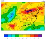
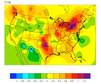
The
original precipitation data are at 4-km resolution on a polar-stereographic
grid. Hourly, 6-hourly and 24-hourly analyses are available. The following image
shows the accumulated 6-h precipitation for the tutorial case.
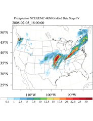
It should be mentioned that the NCEP Stage IV archived data is in GRIB1
format and it cannot be ingested into the WRFDA directly. A tool “CONVERTER” is provided to
reformat GRIB1 observations into the WRFDA-readable ASCII format. It can be
downloaded from the WRFDA users page at http://www2.mmm.ucar.edu/wrf/users/wrfda/download/CONVERTER.gz. The NCEP GRIB libraries, w3 and g2 are required to compile the
CONVERTER. These libraries are available for download from NCEP at http://www.nco.ncep.noaa.gov/pmb/codes/GRIB2/. The output file to the CONVERTER is named in the format ob.rain.yyyymmddhh.xxh; The 'yyyymmddhh' in the file
name is the ending hour of the accumulation period, and 'xx' (=01,06 or 24)
is the accumulating time period.
For users wishing to use their own observations instead of NCEP Stage IV, it is the user’s responsibility to write a Fortran main program and call subroutine writerainobs (in write_rainobs.f90) to generate their own precipitation data. For more information please refer to the README file in the CONVERTER directory.
b. Running WRFDA 4D-Var with precipitation
observations
WRFDA 4D-Var is
able to assimilate hourly, 3-hourly and 6-hourly precipitation data. According to experiments
and related scientific papers, 6-hour precipitation accumulations are the ideal observations to be
assimilated, as this leads to better results than directly assimilating hourly
data.
The tutorial example is for assimilating 6-hour accumulated precipitation. In your working directory, link all the necessary files as follows,
> ln
-fs $WRFDA_DIR/var/da/da_wrfvar.exe .
> ln
-fs $DAT_DIR/rc/2008020512/wrfinput_d01 .
> ln
-fs $DAT_DIR/rc/2008020512/wrfbdy_d01 .
> ln
-fs wrfinput_d01 fg
> ln
-fs $DAT_DIR/be/be.dat .
> ln
-fs $WRFDA_DIR/run/LANDUSE.TBL ./LANDUSE.TBL
> ln
-fs $DAT_DIR/ob/2008020518/ob.rain.2008020518.06h ob07.rain
Note: The reason why the observation ob.rain.2008020518.06h is linked as ob07.rain will be explained in section d.
Edit namelist.input and pay special attention to &wrfvar1 and &wrfvar4 for precipitation-related options.
&wrfvar1
var4d=true,
var4d_lbc=true,
var4d_bin=3600,
var4d_bin_rain=21600,
……
/
……
&wrfvar4
use_rainobs=true,
thin_rainobs=true,
thin_mesh_conv=30*20.,
/
Then, run 4D-Var in serial or parallel mode,
>./da_wrfvar.exe >&! wrfda.log
c. Namelist variables to control
precipitation assimilation
var4d_bin_rain
Precipitation
observation sub-window length for 4D-Var. It does not need to be consistent with
var4d_bin.
thin_rainobs
Logical, TRUE will perform thinning on precipitation data.
thin_mesh_conv
Specify thinning mesh size (in km)
d. Properly linking observation files
In section b, ob.rain.2008020518.06h is linked as ob07.rain. The number 07 is assigned according to the following rule:
x=i*(var4d_bin_rain/var4d_bin)+1,
Here, i is the sequence number of the observation.
for x<10,
the observation file should be renamed as ob0x.rain;
for x>=10, it should be renamed as obx.rain
In the example above, 6-hour accumulated precipitation data is assimilated in 6-hour time window. In the namelist, values should be set at var4d_bin=3600 and var4d_bin_rain=21600, and there is one observation file (i.e., i=1) in the time window, Thus the value of x is 7. The file ob.rain.2008020518.06h should be renamed as ob07.rain.
Let us take another example for how to rename observation files for 3-hourly precipitation data in 6-hour time window. The sample namelist is as follows,
&wrfvar1
var4d=true,
var4d_lbc=true,
var4d_bin=3600,
var4d_bin_rain=10800,
……
/
There are two observation files, ob.rain.2008020515.03h and ob.rain.2008020518.03h. For the first file (i=1) ob.rain.2008020515.03h, it should be renamed as ob04.rain,and the second file (i=2) renamed as ob07.rain.
Updating WRF Boundary Conditions
There are three input files: WRFDA analysis, wrfinput, and wrfbdy files from WPS/real.exe, and a namelist file: parame.in for running da_update_bc.exe for domain-1. Before running an NWP forecast using the WRF-model with WRFDA analysis, update the values and tendencies for each predicted variable in the first time period, in the lateral boundary condition file. Domain-1 (wrfbdy_d01) must be updated to be consistent with the new WRFDA initial condition (analysis). This is absolutely essential. Moreover, in the cycling-run mode (warm-start), the lower boundary in the WRFDA analysis file also needs to be updated based on the information from the wrfinput file, generated by WPS/real.exe at analysis time.
For nested domains, domain-2, domain-3, etc., the lateral boundaries are provided by their parent domains, so no lateral boundary update is needed for these domains; but the low boundaries in each of the nested domains’ WRFDA analysis files still need to be updated. In these cases, you must set the namelist variable, domain_id > 1 (default is 1 for domain-1), and no wrfbdy_d01file needs to be provided to the namelist variable wrf_bdy_file.
This procedure is performed by the WRFDA utility called da_updated_bc.exe, and is located in $WRFDA_DIR/var/build.
To run da_update_bc.exe, follow the steps below:
> cd
$WRFDA_DIR/var/test/update_bc
> cp
–p $DAT_DIR/rc/2008020512/wrfbdy_d01 .
(IMPORTANT: make a copy of wrfbdy_d01, as the wrf_bdy_file will be overwritten by da_update_bc.exe)
> vi
parame.in
&control_param
da_file = './wrfvar_output'
da_file_02 =
‘./ana02’
wrf_bdy_file = './wrfbdy_d01'
wrf_input =
'$DAT_DIR/rc/2008020512/wrfinput_d01'
domain_id = 1
cycling = .false. (set to .true. if first guess comes from a previous WRF forecast.)
debug =
.true.
low_bdy_only = .false.
update_lsm = .false.
var4d_lbc =
.false.
/
> ln
–sf $WRFDA_DIR/var/da/da_update_bc.exe .
>
./da_update_bc.exe
At this stage, you should have the files wrfvar_output and wrfbdy_d01 in your WRFDA working directory. They are the WRFDA updated initial condition and boundary condition for any subsequent WRF model runs. To use, link a copy of wrfvar_output and wrfbdy_d01 to wrfinput_d01 and wrfbdy_d01, respectively, in your WRF working directory.
If you activate the var4d_lbc option in a WRF 4D-Var run, you should also
copy/link the ana02 file from the WRFDA working directory to the da_update_bc working directory and set the var4d_lbc variable to TRUE in parame.in.
Starting with V3.2, some changes
were made to da_update_bc to address some issues related to
sea-ice and snow change during cycling runs, and radiance data assimilation.
The new settings in parame.in are introduced as follows:
Note: for backward compatibility, the pre-V3.2 parame.in, mentioned above, still works with V3.2+ da_update_bc.
&control_param
da_file = '../tutorial/wrfvar_output'
da_file_02
= ‘./ana02’
wrf_bdy_file = './wrfbdy_d01'
wrf_input =
'$DAT_DIR/rc/2008020512/wrfinput_d01'
domain_id = 1
debug = .true.
update_lateral_bdy = .true.
update_low_bdy = .true.
update_lsm = .false.
iswater = 16
var4d_lbc = .false.
/
update_lateral_bdy is required only for domain 1.
update_low_bdy is needed for
all domains if running in cycling mode.
iswater (water point index) is 16 for USGS
LANDUSE and 17 for MODIS LANDUSE.
If in cycling mode (especially if you are doing radiance data assimilation and there are
SEA ICE and SNOW in your domain), it is recommended that before you run WRFDA, you run da_update_bc.exe with the
following namelist options:
update_lateral_bdy = .false.
update_low_bdy = .true.
This creates a lower-boundary updated first guess (da_file will be overwritten by da_update_bc). Then, after WRFDA has finished, run da_update_bc.exe again with the following namelist options:
update_lateral_bdy = .true.
update_low_bdy = .false.
This updates the lateral boundary
conditions (wrf_bdy_file will be overwritten by da_update_bc).
Running gen_be
Starting with WRFDA version 3.1, users have three choices to define the background error covariance (BE). We call them CV3, CV5, and CV6 . With CV3 and CV5, the background errors are applied to the same set of the control variables, stream function, unbalanced potential velocity, unbalanced temperature, unbalanced surface pressure, and pseudo-relative-humidity. However, for CV6 the moisture control variable is the unbalanced part of pseudo-relative-humidity. With CV3, the control variables are in physical space while with CV5 and CV6, the control variables are in eigenvector space. The major difference between these two kinds of BE is the vertical covariance; CV3 uses the vertical recursive filter to model the vertical covariance but CV5 and CV6 use an empirical orthogonal function (EOF) to represent the vertical covariance. The recursive filters to model the horizontal covariance are also different with these BEs. We have not conducted the systematic comparison of the analyses based on these BEs. However, CV3 (a BE file provided with our WRFDA system) is a global BE and can be used for any regional domain, while CV5 and CV6 BE’s are domain-dependent, which should be generated based on the forecast data from the same domain. At this time, it is hard to tell which BE is better; the impact on analysis may vary from case to case.
CV3 is the NCEP background error covariance. It is estimated in grid space by what has become known as the NMC method (Parrish and Derber 1992) . The statistics are estimated with the differences of 24 and 48-hour GFS forecasts with T170 resolution, valid at the same time for 357 cases, distributed over a period of one year. Both the amplitudes and the scales of the background error have to be tuned to represent the forecast error in the estimated fields. The statistics that project multivariate relations among variables are also derived from the NMC method.
The variance of each variable, and the variance of its second derivative, are used to estimate its horizontal scales. For example, the horizontal scales of the stream function can be estimated from the variance of the vorticity and stream function.
The vertical scales are estimated with the vertical correlation of each variable. A table is built to cover the range of vertical scales for the variables. The table is then used to find the scales in vertical grid units. The filter profile and the vertical correlation are fitted locally. The scale of the best fit from the table is assigned as the scale of the variable at that vertical level for each latitude. Note that the vertical scales are locally defined so that the negative correlation further away, in the vertical direction, is not included.
Theoretically, CV3 BE is a generic background error statistics file, which can be used for any case. It is quite straightforward to use CV3 in your own case. To use the CV3 BE file in your case, set cv_options=3 in &wrfvar7 in namelist.input in your working directory, and use the be.dat is located in WRFDA/var/run/be.dat.cv3.
To use CV5 or CV6 background error covariance, it is necessary to generate your domain-specific background error statistics with the gen_be utility. The background error statistics file, supplied with the tutorial test case, can NOT be used for your applications.
The Fortran main programs for gen_be can be found in WRFDA/var/gen_be. The executables of gen_be should have been created when you compiled the WRFDA code (as described earlier). The scripts to run these codes are in WRFDA/var/scripts/gen_be.
The input data for gen_be are WRF forecasts, which are used to generate model perturbations, used as a proxy for estimates of forecast error. For the NMC-method, the model perturbations are differences between forecasts (e.g. T+24 minus T+12 is typical for regional applications, T+48 minus T+24 for global) valid at the same time. Climatological estimates of background error may then be obtained by averaging these forecast differences over a period of time (e.g. one month). Given input from an ensemble prediction system (EPS), the inputs are the ensemble forecasts, and the model perturbations created are the transformed ensemble perturbations. The gen_be code has been designed to work with either forecast difference or ensemble-based perturbations. The former is illustrated in this tutorial example.
It is important to include forecast differences, from at least 00Z and 12Z through the period, to remove the diurnal cycle (i.e. do not run gen_be using just 00Z or 12Z model perturbations alone).
The inputs to gen_be are netCDF WRF forecast output ("wrfout") files at specified forecast ranges. To avoid unnecessary large single data files, it is assumed that all forecast ranges are output to separate files. For example, if we wish to calculate BE statistics using the NMC-method with (T+24)-(T+12) forecast differences (default for regional) then by setting the WRF namelist.input options history_interval=720, and frames_per_outfile=1 we get the necessary output datasets. Then the forecast output files should be arranged as follows: directory name is the forecast initial time, time info in the file name is the forecast valid time. 2008020512/wrfout_d01_2008-02-06_00:00:00 means a 12-hour forecast valid at 2008020600, initialized at 2008020512.
Example dataset for a test case (90 x 60 x 41 gridpoints) can be downloaded from http://www2.mmm.ucar.edu/wrf/users/wrfda/download/testdata.html. Untar the gen_be_forecasts_20080205.tar.gz file. You will have:
>ls $FC_DIR
-rw-r--r-- 1
users 11556492
2008020512/wrfout_d01_2008-02-06_00:00:00
-rw-r--r-- 1
users 11556492
2008020512/wrfout_d01_2008-02-06_12:00:00
-rw-r--r-- 1
users 11556492
2008020600/wrfout_d01_2008-02-06_12:00:00
-rw-r--r-- 1
users 11556492
2008020600/wrfout_d01_2008-02-07_00:00:00
-rw-r--r-- 1
users 11556492
2008020612/wrfout_d01_2008-02-07_00:00:00
-rw-r--r-- 1
users 11556492
2008020612/wrfout_d01_2008-02-07_12:00:00
In the above example, only 1 day (12Z 05 Feb to 12Z 06 Feb. 2002) of forecasts, every 12 hours is supplied to gen_be_wrapper to estimate forecast error covariance. It is only for demonstration. The minimum number of forecasts required depends on the application, number of grid points, etc. Month-long (or longer) datasets are typical for the NMC-method. Generally, at least a 1-month dataset should be used.
Under WRFDA/var/scripts/gen_be, gen_be_wrapper.ksh is used to generate the BE data. The following variables need to be set to fit your case:
export
WRFVAR_DIR=/users/noname/work/code/trunk/phoenix_g95_opt/WRFDA
export
START_DATE=2008020612 # the first
perturbation valid date
export
END_DATE=2008020700 # the last
perturbation valid date
export
NUM_LEVELS=40 # e_vert - 1
export
BIN_TYPE=5
export FC_DIR=/users/noname/work/exps/friendlies/expt/fc
# where wrf forecasts are
export
RUN_DIR=/users/noname/work/exps/friendlies/gen_be${BIN_TYPE}
Note: The START_DATE and END_DATE are perturbation valid dates. As shown in the forecast list above, when you have 24-hour and 12-hour forecasts initialized at 2008020512, through 2008020612, the first and final forecast difference valid dates are 2008020612 and 2008020700, respectively.
Note: The forecast dataset should be located in $FC_DIR. Then type:
>
gen_be_wrapper.ksh
Once the gen_be_wrapper.ksh run is completed, the be.dat can be found under the $RUN_DIR directory.
To get a clear idea about what is included in be.dat, the script gen_be_plot_wrapper.ksh may be used. This plots various data in be.dat; for example: