Chapter 6: WRFDA

Chapter 6: WRF Data Assimilation

Introduction
Installing WRFDA for 3D-Var Run
Installing WRFPLUS and WRFDA for 4D-Var Run
Running Observation Preprocessor (OBSPROC)
Running WRFDA
Radiance Data Assimilation in WRFDA
Radar Data Assimilation in WRFDA
Precipitation Data Assimilation in WRFDA 4D-Var
Updating WRF Boundary Conditions
Background Error and running GEN_BE
Additional WRFDA Exercises
WRFDA Diagnostics
Generating ensembles with RANDOMCV
Hybrid Data Assimilation
ETKF Data Assimilation
Description of Namelist Variables

Introduction

Data assimilation is the technique by which observations are combined with an NWP product (the first guess or background forecast) and their respective error statistics to provide an improved estimate (the analysis) of the atmospheric (or oceanic, Jovian, etc.) state. Variational (Var) data assimilation achieves this through the iterative minimization of a prescribed cost (or penalty) function. Differences between the analysis and observations/first guess are penalized (damped) according to their perceived error. The difference between three-dimensional (3D-Var) and four-dimensional (4D-Var) data assimilation is the use of a numerical forecast model in the latter.

The MMM Laboratory of NCAR supports a unified (global/regional, multi-model, 3/4D-Var) model-space data assimilation system (WRFDA) for use by the NCAR staff and collaborators, and is also freely available to the general community, together with further documentation, test results, plans etc., from the WRFDA web-page (http://www2.mmm.ucar.edu/wrf/users/wrfda/index.html).

Various components of the WRFDA system are shown in blue in the sketch below, together with their relationship with the rest of the WRF system.

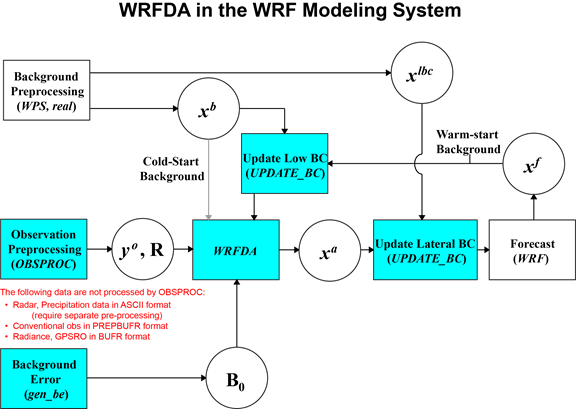
x^b first guess, either from a previous WRF forecast or from WPS/real.exe output.

x^lbc lateral boundary from WPS/real.exe output.

x^a analysis from the WRFDA data assimilation system.

x^f WRF forecast output.

y^o observations processed by OBSPROC. (note: PREPBUFR input, radar, radiance, and rainfall data do not go through OBSPROC)

B₀ background error statistics from generic BE data (CV3) or gen_be.

R observational and representative error statistics.

In this chapter, you will learn how to install and run the various components of the WRFDA system. For training purposes, you are supplied with a test case, including the following input data:

· observation files,

· a netCDF background file (WPS/real.exe output, the first guess of the analysis)

· background error statistics (estimate of errors in the background file).

This tutorial dataset can be downloaded from the WRFDA Users Page (http://www2.mmm.ucar.edu/wrf/users/wrfda/download/testdata.html), and will be described later in more detail. In your own work, however, you will have to create all these input files yourself. See the section “Running Observation Preprocessor” for creating your observation files. See the section “Background Error and running GEN_BE” for generating your background error statistics file, if you want to use cv_options=5, 6, or 7.

Before using your own data, we suggest that you start by running through the WRFDA- related programs using the supplied test case. This serves two purposes: First, you can learn how to run the programs with data we have tested ourselves, and second you can test whether your computer is capable of running the entire data assimilation system. After you have done the tutorial, you can try running other, more computationally intensive case studies, and experimenting with some of the many namelist variables.

WARNING: It is impossible to test every permutation of computer, compiler, number of processors, case, namelist option, etc. for every WRFDA release. The namelist options that are supported are indicated in the “WRFDA/var/README.namelist”, and these are the default options.

Hopefully, our test cases will prepare you for the variety of ways in which you may wish to run your own WRFDA experiments. Please inform us about your experiences.

As a professional courtesy, we request that you include the following references in any publication that uses any component of the community WRFDA system:

Barker, D.M., W. Huang, Y.R. Guo, and Q.N. Xiao., 2004: A Three-Dimensional (3DVAR) Data Assimilation System For Use With MM5: Implementation and Initial Results. Mon. Wea. Rev., 132, 897-914.

Huang, X.Y., Q. Xiao, D.M. Barker, X. Zhang, J. Michalakes, W. Huang, T. Henderson, J. Bray, Y. Chen, Z. Ma, J. Dudhia, Y. Guo, X. Zhang, D.J. Won, H.C. Lin, and Y.H. Kuo, 2009: Four-Dimensional Variational Data Assimilation for WRF: Formulation and Preliminary Results. Mon. Wea. Rev., 137, 299–314.

Barker, D., X.-Y. Huang, Z. Liu, T. Auligné, X. Zhang, S. Rugg, R. Ajjaji, A. Bourgeois, J. Bray, Y. Chen, M. Demirtas, Y.-R. Guo, T. Henderson, W. Huang, H.-C. Lin, J. Michalakes, S. Rizvi, and X. Zhang, 2012: The Weather Research and Forecasting Model's Community Variational/Ensemble Data Assimilation System: WRFDA. Bull. Amer. Meteor. Soc., 93, 831–843.

Running WRFDA requires a Fortran 90 compiler. The WRFDA system can be compiled on the following platforms: Linux (ifort, gfortran, pgf90), Macintosh (gfortran, ifort), IBM (xlf), and SGI Altix (ifort). Please let us know if this does not meet your requirements, and we will attempt to add other machines to our list of supported architectures, as resources allow. Although we are interested in hearing about your experiences in modifying compiler options, we do not recommend making changes to the configure file used to compile WRFDA.

Installing WRFDA for 3D-Var Run

a. Obtaining WRFDA Source Code

Users can download the WRFDA source code from http://www2.mmm.ucar.edu/wrf/users/wrfda/download/get_source.html.

Note: Although the WRFDA package also contains the WRF source code, they can not be built together. WRF should be downloaded and compiled separately.

After the tar file is unzipped (gunzip WRFDAV3.8.TAR.gz) and untarred (tar -xf WRFDAV3.8.TAR), the directory WRFDA should be created. This directory contains the WRFDA source, external libraries, and fixed files. The following is a list of the system components and content for each subdirectory:

Directory Name	Content
var/da	WRFDA source code
var/run	Fixed input files required by WRFDA, such as background error covariance, radiance-related files, CRTM coefficients and VARBC.in
var/external	Libraries needed by WRFDA, includes CRTM, BUFR, LAPACK, BLAS
var/obsproc	OBSPROC source code, namelist, and observation error files
var/gen_be	Source code of gen_be, the utility to create background error statistics files
var/build	Builds all .exe files.

b. Compile WRFDA and Libraries

Some external libraries (e.g., LAPACK, BLAS, and NCEP BUFR) are included in the WRFDA tar file. To compile the WRFDA code, the only mandatory library is the netCDF library. You should set an environment variable NETCDF to point to the directory where your netCDF library is installed

> setenv NETCDF your_netcdf_path

The source code for BUFRLIB 10.2.3 (with minor modifications) is included in the WRFDA tar file, and is compiled automatically. This library will be used for assimilating files in PREPBUFR and NCEP BUFR format.

Starting with WRFDA version 3.8, AMSR2 data can be assimilated in HDF5 format, which requires the use of HDF5 libraries. If you wish to make use of this capability, you should ensure that HDF5 libraries are installed on your system (or download and install them yourself; the source code is available from https://www.hdfgroup.org/HDF5/). To use HDF5 in WRFDA, you should set the environment variable “HDF5” to the parent path of your HDF5 build:

> setenv HDF5 your_hdf5_path

The HDF5 path should contain the directories “include” and “lib”.

For some platforms, you may have to also add the HDF5 “lib” directory to your environment variable LD_LIBRARY_PATH:

> setenv LD_LIBRARY_PATH ${LD_LIBRARY_PATH}:your_hdf5_path/lib

If satellite radiance data are to be used, a Radiative Transfer Model (RTM) is required. The current RTM versions that WRFDA supports are CRTM V2.1.3 and RTTOV V11.1–11.3 .

The CRTM V2.1.3 source code is included in the WRFDA tar file. To compile the CRTM libraries, set the “CRTM” environment variable:

> setenv CRTM 1

If the user wishes to use RTTOV, download and install the RTTOV v11 library before compiling WRFDA. This library can be downloaded from http://nwpsaf.eu/deliverables/rtm/index.html. The RTTOV libraries must be compiled with the “emis_atlas” option in order to work with WRFDA; see the RTTOV “readme.txt” for instructions on how to do this. After compiling RTTOV (see the RTTOV documentation for detailed instructions), set the “RTTOV” environment variable to the path where the lib directory resides. For example, if the library files can be found in /usr/local/rttov11/gfortran/lib/librttov11.*.a, you should set RTTOV as:

> setenv RTTOV /usr/local/rttov11/gfortran

Note: Make sure the required libraries were all compiled using the same compiler that will be used to build WRFDA, since the libraries produced by one compiler may not be compatible with code compiled with another.

Assuming all required libraries are available and the WRFDA source code is ready, you can start to build WRFDA using the following steps:

Enter the WRFDA directory and run the configure script:

> cd WRFDA
> ./configure wrfda

A list of configuration options should appear. Each option combines an operating system, a compiler type, and a parallelism option. Since the configuration script doesn’t check which compilers are actually installed on your system, be sure to select only among the options that you have available to you. The available parallelism options are single-processor (serial), shared-memory parallel (smpar), distributed-memory parallel (dmpar), and distributed-memory with shared-memory parallel (sm+dm). However, shared-memory (smpar and sm+dm) options are not supported as of WRFDA Version 3.8, so we do not recommend selecting any of these options.

For example, on a Linux machine such as NCAR’s Yellowstone, the above steps will look similar to the following:

checking for perl5... no

checking for perl... found /usr/bin/perl (perl)

Will use NETCDF in dir: /glade/apps/opt/netcdf/4.3.0/gnu/4.8.2/

Will use HDF5 in dir: /glade/u/apps/opt/hdf5/1.8.12/gnu/4.8.2/

PHDF5 not set in environment. Will configure WRF for use without.

Will use 'time' to report timing information

$JASPERLIB or $JASPERINC not found in environment, configuring to build without grib2 I/O...

------------------------------------------------------------------------

Please select from among the following Linux x86_64 options:

1. (serial) 2. (smpar) 3. (dmpar) 4. (dm+sm) PGI (pgf90/gcc)

5. (serial) 6. (smpar) 7. (dmpar) 8. (dm+sm) PGI (pgf90/pgcc): SGI MPT

9. (serial) 10. (smpar) 11. (dmpar) 12. (dm+sm) PGI (pgf90/gcc): PGI accelerator

13. (serial) 14. (smpar) 15. (dmpar) 16. (dm+sm) INTEL (ifort/icc)

17. (dm+sm) INTEL (ifort/icc): Xeon Phi (MIC architecture)

18. (serial) 19. (smpar) 20. (dmpar) 21. (dm+sm) INTEL (ifort/icc): Xeon (SNB with AVX mods)

22. (serial) 23. (smpar) 24. (dmpar) 25. (dm+sm) INTEL (ifort/icc): SGI MPT

26. (serial) 27. (smpar) 28. (dmpar) 29. (dm+sm) INTEL (ifort/icc): IBM POE

30. (serial) 31. (dmpar) PATHSCALE (pathf90/pathcc)

32. (serial) 33. (smpar) 34. (dmpar) 35. (dm+sm) GNU (gfortran/gcc)

36. (serial) 37. (smpar) 38. (dmpar) 39. (dm+sm) IBM (xlf90_r/cc_r)

40. (serial) 41. (smpar) 42. (dmpar) 43. (dm+sm) PGI (ftn/gcc): Cray XC CLE

44. (serial) 45. (smpar) 46. (dmpar) 47. (dm+sm) CRAY CCE (ftn/cc): Cray XE and XC

48. (serial) 49. (smpar) 50. (dmpar) 51. (dm+sm) INTEL (ftn/icc): Cray XC

52. (serial) 53. (smpar) 54. (dmpar) 55. (dm+sm) PGI (pgf90/pgcc)

56. (serial) 57. (smpar) 58. (dmpar) 59. (dm+sm) PGI (pgf90/gcc): -f90=pgf90

60. (serial) 61. (smpar) 62. (dmpar) 63. (dm+sm) PGI (pgf90/pgcc): -f90=pgf90

64. (serial) 65. (smpar) 66. (dmpar) 67. (dm+sm) INTEL (ifort/icc): HSW/BDW

68. (serial) 69. (smpar) 70. (dmpar) 71. (dm+sm) INTEL (ifort/icc): KNL MIC

Enter selection [1-71] : 34

------------------------------------------------------------------------

Configuration successful!

------------------------------------------------------------------------

... ...

After entering the option that corresponds to your machine/compiler combination, the configure script should print the message “Configuration successful!” followed by a large amount of configuration information. Depending on your system, you may see a warning message mentioning that some Fortran 2003 features have been removed: this message is normal and can be ignored. However, if you see a message “One of compilers testing failed! Please check your compiler”, configuration has probably failed, and you should make sure you have selected the correct option.

After running the configuration script and choosing a compilation option, a configure.wrf file will be created. Because of the variety of ways that a computer can be configured, if the WRFDA build ultimately fails, there is a chance that minor modifications to the configure.wrf file may be needed.

To compile WRFDA, type

> ./compile all_wrfvar >& compile.out

Successful compilation will produce 44 executables: 43 of which are in the var/build directory and linked in the var/da directory, with the 44th, obsproc.exe, found in the var/obsproc/src directory. You can list these executables by issuing the command:

>ls -l var/build/*exe var/obsproc/src/obsproc.exe

-rwxr-xr-x 1 user 885143 Apr 4 17:22 var/build/da_advance_time.exe

-rwxr-xr-x 1 user 1162003 Apr 4 17:24 var/build/da_bias_airmass.exe

-rwxr-xr-x 1 user 1143027 Apr 4 17:23 var/build/da_bias_scan.exe

-rwxr-xr-x 1 user 1116933 Apr 4 17:23 var/build/da_bias_sele.exe

-rwxr-xr-x 1 user 1126173 Apr 4 17:23 var/build/da_bias_verif.exe

-rwxr-xr-x 1 user 1407973 Apr 4 17:23 var/build/da_rad_diags.exe

-rwxr-xr-x 1 user 1249431 Apr 4 17:22 var/build/da_tune_obs_desroziers.exe

-rwxr-xr-x 1 user 1186368 Apr 4 17:24 var/build/da_tune_obs_hollingsworth1.exe

-rwxr-xr-x 1 user 1083862 Apr 4 17:24 var/build/da_tune_obs_hollingsworth2.exe

-rwxr-xr-x 1 user 1193390 Apr 4 17:24 var/build/da_update_bc_ad.exe

-rwxr-xr-x 1 user 1245842 Apr 4 17:23 var/build/da_update_bc.exe

-rwxr-xr-x 1 user 1492394 Apr 4 17:24 var/build/da_verif_grid.exe

-rwxr-xr-x 1 user 1327002 Apr 4 17:24 var/build/da_verif_obs.exe

-rwxr-xr-x 1 user 26031927 Apr 4 17:31 var/build/da_wrfvar.exe

-rwxr-xr-x 1 user 1933571 Apr 4 17:23 var/build/gen_be_addmean.exe

-rwxr-xr-x 1 user 1944047 Apr 4 17:24 var/build/gen_be_cov2d3d_contrib.exe

-rwxr-xr-x 1 user 1927988 Apr 4 17:24 var/build/gen_be_cov2d.exe

-rwxr-xr-x 1 user 1945213 Apr 4 17:24 var/build/gen_be_cov3d2d_contrib.exe

-rwxr-xr-x 1 user 1941439 Apr 4 17:24 var/build/gen_be_cov3d3d_bin3d_contrib.exe

-rwxr-xr-x 1 user 1947331 Apr 4 17:24 var/build/gen_be_cov3d3d_contrib.exe

-rwxr-xr-x 1 user 1931820 Apr 4 17:24 var/build/gen_be_cov3d.exe

-rwxr-xr-x 1 user 1915177 Apr 4 17:24 var/build/gen_be_diags.exe

-rwxr-xr-x 1 user 1947942 Apr 4 17:24 var/build/gen_be_diags_read.exe

-rwxr-xr-x 1 user 1930465 Apr 4 17:24 var/build/gen_be_ensmean.exe

-rwxr-xr-x 1 user 1951511 Apr 4 17:24 var/build/gen_be_ensrf.exe

-rwxr-xr-x 1 user 1994167 Apr 4 17:24 var/build/gen_be_ep1.exe

-rwxr-xr-x 1 user 1996438 Apr 4 17:24 var/build/gen_be_ep2.exe

-rwxr-xr-x 1 user 2001400 Apr 4 17:24 var/build/gen_be_etkf.exe

-rwxr-xr-x 1 user 1942988 Apr 4 17:24 var/build/gen_be_hist.exe

-rwxr-xr-x 1 user 2021659 Apr 4 17:24 var/build/gen_be_stage0_gsi.exe

-rwxr-xr-x 1 user 2012035 Apr 4 17:24 var/build/gen_be_stage0_wrf.exe

-rwxr-xr-x 1 user 1973193 Apr 4 17:24 var/build/gen_be_stage1_1dvar.exe

-rwxr-xr-x 1 user 1956835 Apr 4 17:24 var/build/gen_be_stage1.exe

-rwxr-xr-x 1 user 1963314 Apr 4 17:24 var/build/gen_be_stage1_gsi.exe

-rwxr-xr-x 1 user 1975042 Apr 4 17:24 var/build/gen_be_stage2_1dvar.exe

-rwxr-xr-x 1 user 1938468 Apr 4 17:24 var/build/gen_be_stage2a.exe

-rwxr-xr-x 1 user 1952538 Apr 4 17:24 var/build/gen_be_stage2.exe

-rwxr-xr-x 1 user 1202392 Apr 4 17:22 var/build/gen_be_stage2_gsi.exe

-rwxr-xr-x 1 user 1947836 Apr 4 17:24 var/build/gen_be_stage3.exe

-rwxr-xr-x 1 user 1928353 Apr 4 17:24 var/build/gen_be_stage4_global.exe

-rwxr-xr-x 1 user 1955622 Apr 4 17:24 var/build/gen_be_stage4_regional.exe

-rwxr-xr-x 1 user 1924416 Apr 4 17:24 var/build/gen_be_vertloc.exe

-rwxr-xr-x 1 user 2057673 Apr 4 17:24 var/build/gen_mbe_stage2.exe

-rwxr-xr-x 1 user 2110993 Apr 4 17:32 var/obsproc/src/obsproc.exe

The main executable for running WRFDA is da_wrfvar.exe. Make sure it has been created after the compilation: it is fairly common that all the executables will be successfully compiled except this main executable. If this occurs, please check the compilation log file carefully for any errors.

The basic gen_be utility for the regional model consists of gen_be_stage0_wrf.exe, gen_be_stage1.exe, gen_be_stage2.exe, gen_be_stage2a.exe, gen_be_stage3.exe, gen_be_stage4_regional.exe, and gen_be_diags.exe.

da_update_bc.exe is used for updating the WRF lower and lateral boundary conditions before and after a new WRFDA analysis is generated. This is detailed in the section on Updating WRF Boundary Conditions.

da_advance_time.exe is a very handy and useful tool for date/time manipulation. Type $WRFDA_DIR/var/build/da_advance_time.exe to see its usage instructions.

obsproc.exe is the executable for preparing conventional observations for assimilation by WRFDA. Its use is detailed in the section on Running Observation Preprocessor.

If you set the environment variable to compile CRTM for radiance assimilation, check $WRFDA_DIR/var/external/crtm_2.1.3/libsrc to ensure that libCRTM.a was generated.

c. Clean Compilation

To remove all object files and executables, type:

./clean

To remove all build files, including configure.wrf, type:

./clean -a

The clean –a command is recommended if your compilation fails, or if the configuration file has been changed and you wish to restore the default settings.

Installing WRFPLUS and WRFDA for 4D-Var Run

If you intend to run WRFDA 4DVAR, it is necessary to have WRFPLUS installed. WRFPLUS contains the adjoint and tangent linear models based on a simplified WRF model, which includes a few simplified physics packages, such as surface drag, large scale condensation and precipitation, and cumulus parameterization.

Note: if you intend to run both 3DVAR and 4DVAR experiments, it is not necessary to compile the code twice. The da_wrfvar.exe executable compiled for 4DVAR can be used for both 3DVAR and 4DVAR assimilation.

To install WRFPLUS:

Get the WRFPLUS zipped tar file from http://www2.mmm.ucar.edu/wrf/users/wrfda/download/wrfplus.html
Unzip and untar the WRFPLUS file, then run the configure script

> gunzip WRFPLUSV3.8.tar.gz

> tar -xf WRFPLUSV3.8.tar

> cd WRFPLUSV3

> ./configure wrfplus

As with 3D-Var, “serial” means single-processor, and “dmpar” means Distributed Memory Parallel (MPI). Be sure to select the same option for WRFPLUS as you will use for WRFDA.

Compile WRFPLUS

> ./compile wrf >& compile.out

> ls -ls main/*.exe

If compilation was successful, you should see the WRFPLUS executable (named wrf.exe):

53292 -rwxr-xr-x 1 user man 54513254 Apr 6 22:43 main/wrf.exe

Finally, set the environment variable WRFPLUS_DIR to the appropriate directory:

>setenv WRFPLUS_DIR ${your_source_code_dir}/WRFPLUSV3

To install WRFDA for the 4D-Var run:

If you intend to use RTTOV to assimilate radiance data, you will need to set the appropriate environment variable at compile time. See the previous 3D-Var section for instructions.

>./configure 4dvar

>./compile all_wrfvar >& compile.out

>ls -ls var/build/*.exe var/obsproc/*.exe

You should see the same 44 executables as are listed in the above 3D-Var section, including da_wrfvar.exe

Running Observation Preprocessor (OBSPROC)

The OBSPROC program reads observations in LITTLE_R format (a text-based format, in use since the MM5 era). We have provided observations for the tutorial case, but for your own applications, you will have to prepare your own observation files. Please see http://www2.mmm.ucar.edu/wrf/users/wrfda/download/free_data.html for the sources of some freely-available observations. Because the raw observation data files have many possible formats, such as ASCII, BUFR, PREPBUFR, MADIS (note: a converter for MADIS data to LITTLE_R is available on the WRFDA website: http://www2.mmm.ucar.edu/wrf/users/wrfda/download/madis.html), and HDF, the free data site also contains instructions for converting the observations to LITTLE_R format. To make the WRFDA system as general as possible, the LITTLE_R format was adopted as an intermediate observation data format for the WRFDA system, however, the conversion of the user-specific source data to LITTLE_R format is the user’s task. A more complete description of the LITTLE_R format, as well as conventional observation data sources for WRFDA, can be found by reading the “Observation Pre-processing” tutorial found at http://www2.mmm.ucar.edu/wrf/users/wrfda/Tutorials/2015_Aug/tutorial_presentations_summer_2015.html, or by referencing Chapter 7 of this User’s Guide.

The purpose of OBSPROC is to:

· Remove observations outside the specified temporal and spatial domains

· Re-order and merge duplicate (in time and location) data reports

· Retrieve pressure or height based on observed information using the hydrostatic assumption

· Check multi-level observations for vertical consistency and superadiabatic conditions

· Assign observation errors based on a pre-specified error file

· Write out the observation file to be used by WRFDA in ASCII or BUFR format

The OBSPROC program (obsproc.exe) should be found under the directory $WRFDA_DIR/var/obsproc/src if “compile all_wrfvar” completed successfully.

If you haven’t already, you should download the tutorial case, which contains example files for all the exercises in this User’s Guide. The case can be found at the WRFDA website (http://www2.mmm.ucar.edu/wrf/users/wrfda/download/testdata.html).

a. Prepare observational data for 3D-Var

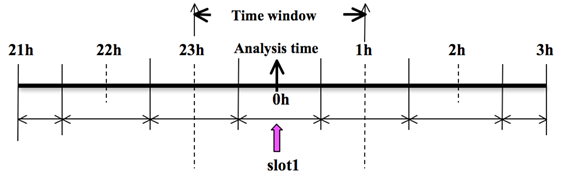
As an example, to prepare the observation file at the analysis time, all the observations in the range ±1h will be processed, which means that (in the example case) the observations between 23h and 1h are treated as the observations at 0h. This is illustrated in the following figure:

OBSPROC requires at least 3 files to run successfully:

· A namelist file (namelist.obsproc)

· An observation error file (obserr.txt)

· One or more observation files

· Optionally, a table for specifying the elevation information for marine observations over the US Great Lakes (msfc.tbl)

The files obserr.txt and msfc.tbl are included in the source code under var/obsproc. To create the required namelist file, we have provided an example file (namelist_obsproc.3dvar.wrfvar-tut) in the var/obsproc directory. Thus, proceed as follows.

> cd $WRFDA_DIR/var/obsproc
> cp namelist.obsproc.3dvar.wrfvar-tut namelist.obsproc

Next, edit the namelist file, namelist.obsproc, to accommodate your experiments. You will likely only need to change variables listed under records 1, 2, 6, 7, and 8. See $WRFDA_DIR/var/obsproc/README.namelist, or the section Description of Namelist Variables for details. You should pay special attention to the record 7 and record 8 variables: these will determine the domain for which observations will be written to the output observation file. Alternatively, if you do not wish to filter the observations spatially, you can set domain_check_h = .false. under &record4.

If you are running the tutorial case, you should copy or link the sample observation file (ob/2008020512/obs.2008020512) to the obsproc directory. Alternatively, you can edit the namelist variable obs_gts_filename to point to the observation file’s full path.

To run OBSPROC, type

> ./obsproc.exe >& obsproc.out

Once obsproc.exe has completed successfully, you will see an observation data file, with the name formatted obs_gts_YYYY-MM-DD_HH:NN:SS.3DVAR, in the obsproc directory. For the tutorial case, this will be obs_gts_2008-02-05_12:00:00.3DVAR. This is the input observation file to WRFDA. It is an ASCII file that contains a header section (listed below) followed by observations. The meanings and format of observations in the file are described in the last six lines of the header section.

TOTAL = 9066, MISS. =-888888.,

SYNOP = 757, METAR = 2416, SHIP = 145, BUOY = 250, BOGUS = 0, TEMP = 86,

AMDAR = 19, AIREP = 205, TAMDAR= 0, PILOT = 85, SATEM = 106, SATOB = 2556,

GPSPW = 187, GPSZD = 0, GPSRF = 3, GPSEP = 0, SSMT1 = 0, SSMT2 = 0,

TOVS = 0, QSCAT = 2190, PROFL = 61, AIRSR = 0, OTHER = 0,

PHIC = 40.00, XLONC = -95.00, TRUE1 = 30.00, TRUE2 = 60.00, XIM11 = 1.00, XJM11 = 1.00,

base_temp= 290.00, base_lapse= 50.00, PTOP = 1000., base_pres=100000., base_tropo_pres= 20000., base_strat_temp= 215.,

IXC = 60, JXC = 90, IPROJ = 1, IDD = 1, MAXNES= 1,

NESTIX= 60,

NESTJX= 90,

NUMC = 1,

DIS = 60.00,

NESTI = 1,

NESTJ = 1,

INFO = PLATFORM, DATE, NAME, LEVELS, LATITUDE, LONGITUDE, ELEVATION, ID.

SRFC = SLP, PW (DATA,QC,ERROR).

EACH = PRES, SPEED, DIR, HEIGHT, TEMP, DEW PT, HUMID (DATA,QC,ERROR)*LEVELS.

INFO_FMT = (A12,1X,A19,1X,A40,1X,I6,3(F12.3,11X),6X,A40)

SRFC_FMT = (F12.3,I4,F7.2,F12.3,I4,F7.3)

EACH_FMT = (3(F12.3,I4,F7.2),11X,3(F12.3,I4,F7.2),11X,3(F12.3,I4,F7.2))

#------------------------------------------------------------------------------#

…… observations ………

Before running WRFDA, you may find it useful to learn more about various types of data that will be processed (e.g., their geographical distribution). This file is in ASCII format and so you can easily view it. For a graphical view of the file's content, there are NCL scripts available which can display the distribution and type of observations. In the WRFDA Tools package (can be downloaded at http://www2.mmm.ucar.edu/wrf/users/wrfda/download/tools.html), the relevant script is located at $TOOLS_DIR/var/graphics/ncl/plot_ob_ascii_loc.ncl. You will need to have NCL installed in your system to use this script; for more information on NCL, the NCAR Command Language, see http://www.ncl.ucar.edu/.

b. Prepare observational data for 4D-Var

To prepare the observation file, for example, at the analysis time 0h for 4D-Var, all observations from 0h to 6h will be processed and grouped in 7 sub-windows (slot1 through slot7) as illustrated in the following figure:

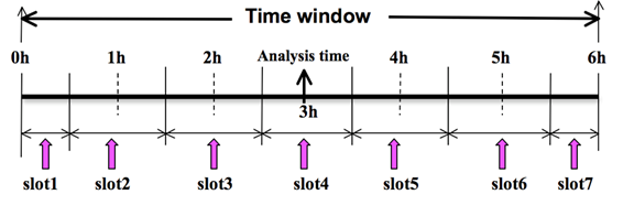
NOTE: The “Analysis time” in the above figure is not the actual analysis time (0h). It indicates the time_analysis setting in the namelist file, which in this example is three hours later than the actual analysis time. The actual analysis time is still 0h.

An example namelist (namelist_obsproc.4dvar.wrfvar-tut) has already been provided in the var/obsproc directory. Thus, proceed as follows:

> cd $WRFDA_DIR/var/obsproc
> cp namelist.obsproc.4dvar.wrfvar-tut namelist.obsproc

In the namelist file, you need to change the following variables to accommodate your experiments. In this tutorial case, the actual analysis time is 2008-02-05_12:00:00, but in the namelist, time_analysis should be set to 3 hours later. The different values of time_analysis, num_slots_past, and time_slots_ahead contribute to the actual times analyzed. For example, if you set time_analysis = 2008-02-05_16:00:00, and set the num_slots_past = 4 and time_slots_ahead=2, the final results will be the same as before.

Edit all the domain settings according to your own experiment; a full list of namelist options and descriptions can be found in the section Description of Namelist Variables. You should pay special attention to the record 7 and record 8 variables: these will determine the domain for which observations will be written to the output observation file. Alternatively, if you do not wish to filter the observations spatially, you can set domain_check_h = .false. under &record4.

To run OBSPROC, type

> obsproc.exe >& obsproc.out

Once obsproc.exe has completed successfully, you will see 7 observation data files, which for the tutorial case are named

obs_gts_2008-02-05_12:00:00.4DVAR

obs_gts_2008-02-05_13:00:00.4DVAR

obs_gts_2008-02-05_14:00:00.4DVAR

obs_gts_2008-02-05_15:00:00.4DVAR

obs_gts_2008-02-05_16:00:00.4DVAR

obs_gts_2008-02-05_17:00:00.4DVAR

obs_gts_2008-02-05_18:00:00.4DVAR

They are the input observation files to WRF 4D-Var.

Running WRFDA

a. Download Test Data

The WRFDA system requires three input files to run:

a) WRF first guess file, output from either WPS/real.exe (cold-start) or a WRF forecast (warm-start)

b) Observations (in ASCII format, PREPBUFR or BUFR for radiance)

c) A background error statistics file (containing background error covariance)

The following table summarizes the above info:

Input Data	Format	Created By
First Guess	NETCDF	WRF Preprocessing System (WPS) and real.exe or WRF
Observations	ASCII (PREPBUFR also possible)	Observation Preprocessor (OBSPROC)
Background Error Statistics	Binary	WRFDA gen_be utility or generic CV3

In the test case, you will store data in a directory defined by the environment variable $DAT_DIR. This directory can be in any location, and it should have read access. Type

> setenv DAT_DIR your_choice_of_dat_dir

Here, your_choice_of_dat_dir is the directory where the WRFDA input data is stored.

If you have not already done so, download the sample data for the tutorial case, valid at 12 UTC 5^thFebruary 2008, from http://www2.mmm.ucar.edu/wrf/users/wrfda/download/testdata.html

Once you have downloaded the WRFDAV3.8-testdata.tar.gz file to $DAT_DIR, extract it by typing

> gunzip WRFDAV3.8-testdata.tar.gz
> tar -xvf WRFDAV3.8-testdata.tar

Now you should find the following four files under “$DAT_DIR”

ob/2008020512/ob.2008020512      # Observation data in “little_r” format
rc/2008020512/wrfinput_d01       # First guess file
rc/2008020512/wrfbdy_d01         # lateral boundary file
be/be.dat                        # Background error file

......

At this point you should have three of the input files (first guess, observations from OBSPROC, and background error statistics files in the directory $DAT_DIR) required to run WRFDA, and have successfully downloaded and compiled the WRFDA code. If this is correct, you are ready to run WRFDA.

b. Run the Case—3D-Var

The data for the tutorial case is valid at 12 UTC 5 February 2008. The first guess comes from the NCEP FNL (Final) Operational Global Analysis data, passed through the WRF-WPS and real.exe programs.

To run WRF 3D-Var, first create and enter into a working directory (for example, $WRFDA_DIR/workdir), and set the environment variable WORK_DIR to this directory (e.g., setenv WORK_DIR $WRFDA_DIR/workdir). Then follow the steps below:

> cd $WORK_DIR

> cp $DAT_DIR/namelist.input.3dvar namelist.input

> ln -sf $WRFDA_DIR/run/LANDUSE.TBL .

> ln -sf $DAT_DIR/rc/2008020512/wrfinput_d01 ./fg

> ln -sf $DAT_DIR/ob/2008020512/obs_gts_2008-02-05_12:00:00.3DVAR ./ob.ascii (note the different name!)

> ln -sf $DAT_DIR/be/be.dat .

> ln -sf $WRFDA_DIR/var/da/da_wrfvar.exe .

Now edit the file namelist.input, which is a very basic namelist for the tutorial test case, and is shown below.

&wrfvar1

var4d=false,

print_detail_grad=false,

&wrfvar2

&wrfvar3

ob_format=2,

&wrfvar4

&wrfvar5

&wrfvar6

max_ext_its=1,

ntmax=50,

orthonorm_gradient=true,

&wrfvar7

cv_options=5,

&wrfvar8

&wrfvar9

&wrfvar10

test_transforms=false,

test_gradient=false,

&wrfvar11

&wrfvar12

&wrfvar13

&wrfvar14

&wrfvar15

&wrfvar16

&wrfvar17

&wrfvar18

analysis_date="2008-02-05_12:00:00.0000",

&wrfvar19

&wrfvar20

&wrfvar21

time_window_min="2008-02-05_11:00:00.0000",

&wrfvar22

time_window_max="2008-02-05_13:00:00.0000",

&time_control

start_year=2008,

start_month=02,

start_day=05,

start_hour=12,

end_year=2008,

end_month=02,

end_day=05,

end_hour=12,

&fdda

&domains

e_we=90,

e_sn=60,

e_vert=41,

dx=60000,

dy=60000,

&dfi_control

&tc

&physics

mp_physics=3,

ra_lw_physics=1,

ra_sw_physics=1,

radt=60,

sf_sfclay_physics=1,

sf_surface_physics=1,

bl_pbl_physics=1,

cu_physics=1,

cudt=5,

num_soil_layers=5,

mp_zero_out=2,

co2tf=0,

&scm

&dynamics

&bdy_control

&grib2

&fire

&namelist_quilt

&perturbation

No edits should be needed if you are running the tutorial case without radiance data. If you plan to use the PREPBUFR-format data, change the ob_format=1 in &wrfvar3 in namelist.input and link the data as ob.bufr,

> ln -fs $DAT_DIR/ob/2008020512/gdas1.t12z.prepbufr.nr ob.bufr

Once you have changed any other necessary namelist variables, run WRFDA 3D-Var:

> da_wrfvar.exe >& wrfda.log

The file wrfda.log (or rsl.out.0000, if run in distributed-memory mode) contains important WRFDA runtime log information. Always check the log after a WRFDA run:

*** VARIATIONAL ANALYSIS ***

DYNAMICS OPTION: Eulerian Mass Coordinate

alloc_space_field: domain 1 , 419050728 bytes allocated

Tile Strategy is not specified. Assuming 1D-Y

WRF TILE 1 IS 1 IE 89 JS 1 JE 59

WRF NUMBER OF TILES = 1

Set up observations (ob)

Using ASCII format observation input

Observation summary

ob time 1

sound 86 global, 86 local

synop 750 global, 750 local

pilot 85 global, 85 local

satem 105 global, 105 local

geoamv 2499 global, 2499 local

airep 216 global, 216 local

gpspw 187 global, 187 local

gpsrf 3 global, 3 local

metar 2408 global, 2408 local

ships 135 global, 135 local

qscat 2126 global, 2126 local

profiler 61 global, 61 local

buoy 247 global, 247 local

sonde_sfc 86 global, 86 local

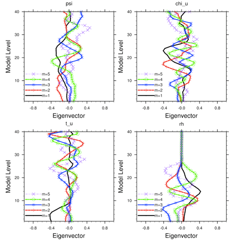
Set up background errors for regional application for cv_options = 5

Using the averaged regression coefficients for unbalanced part

WRFDA dry control variables are: psi, chi_u, t_u and ps_u

Humidity control variable is rh

Vertical truncation for psi = 16( 99.00%)

Vertical truncation for chi_u = 21( 99.00%)

Vertical truncation for t_u = 28( 99.00%)

Vertical truncation for rh = 21( 99.00%)

Scaling: var, len, ds: 0.100000E+01 0.100000E+01 0.600000E+05

Calculate innovation vector(iv)

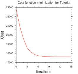
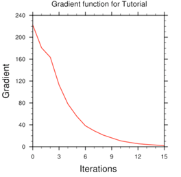
Minimize cost function using CG method

Starting outer iteration : 1

Starting cost function: 2.899074954207616D+04, Gradient= 4.257569431368675D+02

For this outer iteration gradient target is: 4.257569431368675D+00

----------------------------------------------------------

Iter Cost Function Gradient Step

1 2.771806953835228D+04 3.839443040010825D+02 1.404189554585295D-02

2 2.607328843808729D+04 3.776030549295726D+02 2.231524424457818D-02

3 2.472259943260248D+04 3.222689578709167D+02 1.894586166646225D-02

4 2.386086652415530D+04 2.434640871750135D+02 1.659455934972616D-02

5 2.327265820675138D+04 2.263256490947211D+02 1.984683869146577D-02

6 2.288387097811670D+04 1.972809202546574D+02 1.518009315679554D-02

7 2.253852621449510D+04 1.766242834719637D+02 1.774649948213140D-02

8 2.219417744229300D+04 1.618922878245313D+02 2.207637224768432D-02

9 2.192368221682242D+04 1.229826464959493D+02 2.064131105434926D-02

10 2.177234151876604D+04 1.098452932230578D+02 2.001234860476772D-02

11 2.165515456004121D+04 9.038821333939826D+01 1.942434459905811D-02

12 2.154905449070163D+04 6.171712290037125D+01 2.597299664471773D-02

13 2.148634583759935D+04 5.900027652146414D+01 3.292654210894269D-02

14 2.144348889336520D+04 5.558586880547042D+01 2.462312123702110D-02

15 2.141094656736842D+04 4.328574339190531D+01 2.106443384244755D-02

16 2.138841979319319D+04 4.623858932948649D+01 2.404580052377259D-02

17 2.137137039364308D+04 2.944845359103514D+01 1.594887052142258D-02

18 2.135801077614940D+04 2.703119452870921D+01 3.081052025436094D-02

19 2.134790283741255D+04 2.000068983535672D+01 2.766700323513679D-02

20 2.134243403434521D+04 1.895724733612341D+01 2.734212914523067D-02

21 2.133743668978750D+04 1.371809418862918D+01 2.781113653579010D-02

22 2.133439013371656D+04 1.232859989163032D+01 3.237811866762183D-02

23 2.133175083687751D+04 9.696878152742697D+00 3.472887512091716D-02

24 2.133033618679966D+04 7.719188785704023D+00 3.008951215120560D-02

25 2.132937372961099D+04 6.171750208439374D+00 3.230487696342357D-02

26 2.132880381311464D+04 5.055452490576116D+00 2.992433741464962D-02

27 2.132819634377840D+04 4.267442341035473D+00 4.753727571760313D-02

28 2.132795798122098D+04 3.559547648716643D+00 2.617777365464800D-02

----------------------------------------------------------

Inner iteration stopped after 28 iterations

Final: 28 iter, J= 2.132795798122041D+04, g= 3.559547648716685D+00

----------------------------------------------------------

Diagnostics

Final cost function J = 21327.96

Total number of obs. = 39820

Final value of J = 21327.95798

Final value of Jo = 18771.08660

Final value of Jb = 2556.87138

Final value of Jc = 0.00000

Final value of Je = 0.00000

Final value of Jp = 0.00000

Final value of Jl = 0.00000

Final J / total num_obs = 0.53561

Jb factor used(1) = 1.00000

Jb factor used(2) = 1.00000

Jb factor used(3) = 1.00000

Jb factor used(4) = 1.00000

Jb factor used(5) = 1.00000

Jb factor used = 1.00000

Je factor used = 1.00000

VarBC factor used = 1.00000

*** WRF-Var completed successfully ***

The file namelist.output.da (which contains the complete namelist settings) will be generated after a successful run of da_wrfvar.exe. The settings appearing in namelist.output.da, but not specified in your namelist.input, are the default values from $WRFDA_DIR/Registry/registry.var.

After successful completion, wrfvar_output (the WRFDA analysis file, i.e. the new initial condition for WRF) should appear in the working directory along with a number of diagnostic files. Text files containing various diagnostics will be explained in the WRFDA Diagnostics section.

To understand the role of various important WRFDA options, try re-running WRFDA by changing different namelist options. For example, try making the WRFDA convergence criterion more stringent. This is achieved by reducing the value of “EPS” to e.g. 0.0001 by adding "EPS=0.0001" in the namelist.input record &wrfvar6. See the section Additional WRFDA exercises for more namelist options.

c. Run the Case—4D-Var

To run WRF 4D-Var, first create and enter a working directory, such as $WRFDA_DIR/workdir. Set the WORK_DIR environment variable (e.g. setenv WORK_DIR $WRFDA_DIR/workdir)

For the tutorial case, the analysis date is 2008020512 and the test data directories are:

> setenv DAT_DIR {directory where data is stored}

> ls –lr $DAT_DIR

ob/2008020512

ob/2008020513

ob/2008020514

ob/2008020515

ob/2008020516

ob/2008020517

ob/2008020518

rc/2008020512

Note: WRFDA 4D-Var is able to assimilate conventional observational data, satellite radiance BUFR data, and precipitation data. The input data format can be PREPBUFR format data or ASCII observation data, processed by OBSPROC.

Now follow the steps below:

1) Link the executable file

> cd $WORK_DIR

> ln -fs $WRFDA_DIR/var/da/da_wrfvar.exe .

2) Link the observational data, first guess, BE and LANDUSE.TBL, etc.

> ln -fs $DAT_DIR/ob/2008020512/ob01.ascii ob01.ascii

> ln -fs $DAT_DIR/ob/2008020513/ob02.ascii ob02.ascii

> ln -fs $DAT_DIR/ob/2008020514/ob03.ascii ob03.ascii

> ln -fs $DAT_DIR/ob/2008020515/ob04.ascii ob04.ascii

> ln -fs $DAT_DIR/ob/2008020516/ob05.ascii ob05.ascii

> ln -fs $DAT_DIR/ob/2008020517/ob06.ascii ob06.ascii

> ln -fs $DAT_DIR/ob/2008020518/ob07.ascii ob07.ascii

> ln -fs $DAT_DIR/rc/2008020512/wrfinput_d01 .

> ln -fs $DAT_DIR/rc/2008020512/wrfbdy_d01 .

> ln -fs wrfinput_d01 fg

> ln -fs $DAT_DIR/be/be.dat .

> ln -fs $WRFDA_DIR/run/LANDUSE.TBL .

> ln -fs $WRFDA_DIR/run/GENPARM.TBL .

> ln -fs $WRFDA_DIR/run/SOILPARM.TBL .

> ln -fs $WRFDA_DIR/run/VEGPARM.TBL .

> ln –fs $WRFDA_DIR/run/RRTM_DATA_DBL RRTM_DATA

3) Copy the sample namelist

> cp $DAT_DIR/namelist.input.4dvar namelist.input

4) Edit necessary namelist variables, link optional files

WRFDA 4D-Var has the capability to consider lateral boundary conditions as control variables as well during minimization. The namelist variable var4d_lbc=true turns on this capability. To enable this option, WRF 4D-Var needs not only the first guess at the beginning of the time window, but also the first guess at the end of the time window.

> ln -fs $DAT_DIR/rc/2008020518/wrfinput_d01 fg02

Please note: WRFDA beginners should not use this option until you have a good understanding of the 4D-Var lateral boundary conditions control. To disable this feature, make sure var4d_lbc in namelist.input is set to false.

If you use PREPBUFR format data, set ob_format=1 in &wrfvar3 in namelist.input. Because 12UTC PREPBUFR data only includes the data from 9UTC to 15UTC, for 4D-Var you should include 18UTC PREPBUFR data as well:

> ln -fs $DAT_DIR/ob/2008020512/gdas1.t12z.prepbufr.nr ob01.bufr

> ln -fs $DAT_DIR/ob/2008020518/gdas1.t18z.prepbufr.nr ob02.bufr

Edit namelist.input to match your experiment settings. The most important namelist variables related to 4D-Var are listed below. Please refer to README.namelist under the $WRFDA_DIR/var directory. A common mistake users make is in the time information settings. The rules are: analysis_date, time_window_min and start_xxx in &time_control should always be equal to each other; time_window_max and end_xxx should always be equal to each other; and run_hours is the difference between start_xxx and end_xxx, which is the length of the 4D-Var time window.

&wrfvar1

var4d=true,

var4d_lbc=false,

var4d_bin=3600,

……
/

……

&wrfvar18

analysis_date="2008-02-05_12:00:00.0000",

……

&wrfvar21

time_window_min="2008-02-05_12:00:00.0000",

……

&wrfvar22

time_window_max="2008-02-05_18:00:00.0000",

……

&time_control

run_hours=6,

start_year=2008,

start_month=02,

start_day=05,

start_hour=12,

end_year=2008,

end_month=02,

end_day=05,

end_hour=18,

interval_seconds=21600,

debug_level=0,

……

5) Run WRF 4D-Var

> cd $WORK_DIR

> ./da_wrfvar.exe >& wrfda.log

4DVAR is much more computationally expensive than 3DVAR, so running may take a while; you can set ntmax to a lower value so that WRFDA uses fewer minimization steps. You can also MPI with multiple processors to speed up the execution:

> mpirun –np 4 ./da_wrfvar.exe >& wrfda.log &

The “mpirun” command may be different depending on your machine. The output logs will be found in files named rsl.out.#### and rsl.error.#### for MPI runs.

Please note: If you utilize the lateral boundary conditions option (var4d_lbc=true), in addition to the analysis at the beginning of the time window (wrfvar_output), the analysis at the end of the time window will also be generated as ana02, which will be used in subsequent updating of boundary conditions before the forecast.

Radiance Data Assimilation in WRFDA

This section gives a brief description for various aspects related to radiance assimilation in WRFDA. Each aspect is described mainly from the viewpoint of usage, rather than more technical and scientific details, which will appear in a separate technical report and scientific paper. Namelist parameters controlling different aspects of radiance assimilation will be detailed in the following sections. It should be noted that this section does not cover general aspects of the assimilation process with WRFDA; these can be found in other sections of chapter 6 of this user’s guide, or other WRFDA documentation.

a. Running WRFDA with radiances

In addition to the basic input files (LANDUSE.TBL, fg, ob.ascii, be.dat) mentioned in the “Running WRFDA” section, the following additional files are required for radiances: radiance data (typically in NCEP BUFR format), radiance_info files, VARBC.in (if you plan on using variational bias correction VARBC, as described in the section on bias correction), and RTM (CRTM or RTTOV) coefficient files.

Edit namelist.input (Pay special attention to &wrfvar4, &wrfvar14, &wrfvar21, and &wrfvar22 for radiance-related options. A very basic namelist.input for running the radiance test case is provided in WRFDA/var/test/radiance/namelist.input)

> ln -sf $DAT_DIR/gdas1.t00z.1bamua.tm00.bufr_d ./amsua.bufr

> ln -sf $DAT_DIR/gdas1.t00z.1bamub.tm00.bufr_d ./amsub.bufr

> ln -sf $WRFDA_DIR/var/run/radiance_info ./radiance_info # (radiance_info is a directory)

> ln -sf $WRFDA_DIR/var/run/VARBC.in ./VARBC.in

(CRTM only) > ln -sf WRFDA/var/run/crtm_coeffs ./crtm_coeffs #(crtm_coeffs is a directory)

(RTTOV only) > ln -sf your_RTTOV_path/rtcoef_rttov11/rttov7pred54L ./rttov_coeffs # (rttov_coeffs is a directory)

Note: You can also specify the path of the “ crtm_coeffs” directory via the namelist; see the following section for more details

See the following sections for more details on each aspect of radiance assimilation.

b. Radiance Data Ingest

Currently, the ingest interface for NCEP BUFR radiance data is implemented in WRFDA. The radiance data are available through NCEP’s public ftp server (ftp://ftp.ncep.noaa.gov/pub/data/nccf/com/gfs/prod/gdas.${yyyymmddhh}) in near real-time (with a 6-hour delay) and can meet requirements for both research purposes and some real-time applications.

As of Version 3.8, WRFDA can read data from NOAA ATOVS instruments (HIRS, AMSU-A, AMSU-B and MHS), EOS Aqua instruments (AIRS, AMSU-A), DMSP instruments (SSMIS), METOP instruments (HIRS, AMSU-A, MHS, IASI), Meteosat instruments (SEVIRI), and JAXA instruments (GCOM-W1). Note that NCEP radiance BUFR files are separated by instrument names (i.e., one file for each type of instrument), and each file contains global radiance (generally converted to brightness temperature) within a 6-hour assimilation window, from multi-platforms. For running WRFDA, users need to rename NCEP corresponding BUFR files (table 1) to hirs3.bufr (including HIRS data from NOAA-15/16/17), hirs4.bufr (including HIRS data from NOAA-18/19, METOP-2), amsua.bufr (including AMSU-A data from NOAA-15/16/18/19, METOP-1 and -2), amsub.bufr (including AMSU-B data from NOAA-15/16/17), mhs.bufr (including MHS data from NOAA-18/19 and METOP-1 and -2), airs.bufr (including AIRS and AMSU-A data from EOS-AQUA) ssmis.bufr (SSMIS data from DMSP-16, AFWA provided) iasi.bufr (IASI data from METOP-1 and -2) and seviri.bufr (SEVIRI data from Meteosat 8-10) for WRFDA filename convention. Note that the airs.bufr file contains not only AIRS data but also AMSU-A, which is collocated with AIRS pixels (1 AMSU-A pixel collocated with 9 AIRS pixels). Users must place these files in the working directory where the WRFDA executable is run. It should also be mentioned that WRFDA reads these BUFR radiance files directly without the use of any separate pre-processing program. All processing of radiance data, such as quality control, thinning, bias correction, etc., is carried out within WRFDA. This is different from conventional observation assimilation, which requires a pre-processing package (OBSPROC) to generate WRFDA readable ASCII files. For reading the radiance BUFR files, WRFDA must be compiled with the NCEP BUFR library (see http://www.nco.ncep.noaa.gov/sib/decoders/BUFRLIB/).

Table 1: NCEP and WRFDA radiance BUFR file naming convention

NCEP BUFR file names	WRFDA naming convention
gdas1.t00z.airsev.tm00.bufr_d	airs.bufr
gdas1.t00z.1bamua.tm00.bufr_d	amsua.bufr
gdas1.t00z.1bamub.tm00.bufr_d	amsub.bufr
gdas1.t00z.atms.tm00.bufr_d	atms.bufr
gdas1.t00z.1bhrs3.tm00.bufr_d	hirs3.bufr
gdas1.t00z.1bhrs4.tm00.bufr_d	hirs4.bufr
gdas1.t00z.mtiasi.tm00.bufr_d	iasi.bufr
gdas1.t00z.1bmhs.tm00.bufr_d	mhs.bufr
gdas1.t00z.sevcsr.tm00.bufr_d	seviri.bufr

Namelist parameters are used to control the reading of corresponding BUFR files into WRFDA. For instance, USE_AMSUAOBS, USE_AMSUBOBS, USE_HIRS3OBS, USE_HIRS4OBS, USE_MHSOBS, USE_AIRSOBS, USE_EOS_AMSUAOBS, USE_SSMISOBS, USE_ATMSOBS, USE_IASIOBS, and USE_SEVIRIOBS control whether or not the respective file is read. These are logical parameters that are assigned to .FALSE. by default; therefore they must be set to .TRUE. to read the respective observation file. Also note that these parameters only control whether the data is read, not whether the data included in the files is to be assimilated. This is controlled by other namelist parameters explained in the next section.

Sources for downloading these and other data can be found on the WRFDA website: http://www2.mmm.ucar.edu/wrf/users/wrfda/download/free_data.html.

Other data formats

Most of the above paragraphs describe NCEP BUFR data, but some of the satellite data supported by WRFDA are in alternate formats. Level-1R AMSR2 data from the JAXA GCOM-W1 satellite are available in HDF5 format, which requires compiling WRFDA with HDF5 libraries, as described in the “Compile WRFDA and Libraries” section.

HDF5 file naming conventions are different than those for BUFR files. For AMSR2 data, WRFDA will look for two files: L1SGRTBR.h5 (brightness temperature) and L2SGCLWLD.h5 (cloud liquid water). Only the brightness temperature file is mandatory. If you have multiple data files for your assimilation window, you should name them L1SGRTBR-01.h5, L1SGRTBR-02.h5, etc. and L2SGCLWLD-01.h5, L2SGCLWLD-02.h5, etc.

c. Radiative Transfer Model

The core component for direct radiance assimilation is to incorporate a radiative transfer model (RTM) into the WRFDA system as one part of observation operators. Two widely used RTMs in the NWP community, RTTOV (developed by ECMWF and UKMET in Europe), and CRTM (developed by the Joint Center for Satellite Data Assimilation (JCSDA) in US), are already implemented in the WRFDA system with a flexible and consistent user interface. WRFDA is designed to be able to compile with or without CRTM or RTTOV by the definition of environment variables “CRTM” and “RTTOV” respectively at compile time (see the “Compile WRFDA and Libraries” section). At runtime the user must select which RTM they intend to use via the namelist parameter RTM_OPTION (1 for RTTOV, the default, and 2 for CRTM).

Both RTMs can calculate radiances for almost all available instruments aboard the various satellite platforms in orbit. An important feature of the WRFDA design is that all data structures related to radiance assimilation are dynamically allocated during running time, according to a simple namelist setup. The instruments to be assimilated are controlled at run-time by four integer namelist parameters: RTMINIT_NSENSOR (the total number of sensors to be assimilated), RTMINIT_PLATFORM (the platforms IDs array to be assimilated with dimension RTMINIT_NSENSOR, e.g., 1 for NOAA, 9 for EOS, 10 for METOP and 2 for DMSP), RTMINIT_SATID (satellite IDs array) and RTMINIT_SENSOR (sensor IDs array, e.g., 0 for HIRS, 3 for AMSU-A, 4 for AMSU-B, etc.). The full list of instrument triplets can be found in the table below:

Instrument	Satellite	Format	(PLATFORM, SATID, SENSOR)
AIRS	EOS-Aqua	BUFR	(9,2,11)
AMSR2	GCOM-W1	HDF5	(29,1,63)
AMSU-A	EOS-Aqua	BUFR	(9,2,3)
AMSU-A	METOP-A	BUFR	(10,2,3)
AMSU-A	NOAA 15–19	BUFR	(1,15–19,3)
AMSU-B	NOAA 15–17	BUFR	(1,15–17,4)
ATMS	Suomi-NPP	BUFR	(17,0,19)
HIRS-3	NOAA 15–17	BUFR	(1,15–17,0)
HIRS-4	METOP-A	BUFR	(10,2,0)
HIRS-4	NOAA 18–19	BUFR	(1,18–19,0)
IASI	METOP-A	BUFR	(10,2,16)
MHS	METOP-A	BUFR	(10,2,15)
MHS	NOAA 18–19	BUFR	(1,18–19,15)
MWHS	FY-3A–FY-3B	Binary	(23,1–2,41)
MWTS	FY-3A–FY-3B	Binary	(23,1–2,40)
SEVIRI	Meteosat 8–10	BUFR	(12,1–3,21)
SSMIS	DMSP 16–18	BUFR	(2,16–18,10)

Here’s an example of this section of the namelist for a user assimilating AMSU-A from NOAA 18–19 and EOS-Aqua, MHS from NOAA 18–19, and AIRS from EOS-Aqua, utilizing CRTM as their RTM:

&wrfvar14

rtminit_nsensor = 6

rtminit_platform = 1, 1, 9, 1, 1,

rtminit_satid = 18, 19, 2, 18, 19, 2

rtminit_sensor = 3, 3, 3, 15, 15, 11

rtm_option = 2,

The instrument triplets (platform, satellite, and sensor ID) in the namelist can be ranked in any order. More detail about the convention of instrument triples can be found in tables 2 and 3 in the RTTOV v11 User’s Guide (http://nwpsaf.eu/deliverables/rtm/docs_rttov11/users_guide_11_v1.4.pdf)

CRTM uses a different instrument-naming method, however, a conversion routine inside WRFDA is implemented such that the user interface remains the same for RTTOV and CRTM, using the same instrument triplet for both.

When running WRFDA with radiance assimilation switched on, a set of RTM coefficient files need to be loaded. For the RTTOV option, RTTOV coefficient files are to be copied or linked to a sub-directory rttov_coeffs/ under the working directory. For the CRTM option, CRTM coefficient files are to be copied or linked to a sub-directory crtm_coeffs/ under the working directory, or the location of this directory can be specified in the namelist:

&wrfvar14

crtm_coef_path = WRFDA/var/run/crtm_coeffs (Can be a relative or absolute path)

Only coefficients for instruments listed in the namelist are needed. Potentially WRFDA can assimilate all sensors as long as the corresponding coefficient files are provided. In addition, necessary developments on the corresponding data interface, quality control, and bias correction are important to make radiance data assimilate properly; however, a modular design of radiance relevant routines already facilitates the addition of more instruments in WRFDA.

The RTTOV package is not distributed with WRFDA, due to licensing restrictions. Users need to follow the instructions at http://nwpsaf.eu/site/software/rttov/ to download the RTTOV source code and supplement coefficient files and the emissivity atlas dataset. Only RTTOV v11 (11.1—11.3) can be used in WRFDA version 3.8, so if you have an older version of RTTOV you must upgrade.

As mentioned in a previous paragraph, the CRTM package is distributed with WRFDA, and is located in $WRFDA_DIR/var/external/crtm_2.1.3. The CRTM code in WRFDA is the same as the source code that users can download from ftp://ftp.emc.ncep.noaa.gov/jcsda/CRTM, with only minor modifications (mainly for ease of compilation).

To use one or both of the above radiative transfer models, you will have to set the appropriate environment variable(s) at compile time. See the section “Compile WRFDA and Libraries” for details.

d. Channel Selection

Channel selection in WRFDA is controlled by radiance ‘info’ files, located in the sub-directory radiance_info, under the working directory. These files are separated by satellites and sensors; e.g., noaa-15-amsua.info, noaa-16-amsub.info, dmsp-16-ssmis.info and so on. An example of 5 channels from noaa-15-amsub.info is shown below. The fourth column is used by WRFDA to control when to use a corresponding channel. Channels with the value “-1” in the fourth column indicate that the channel is “not assimilated,” while the value “1” means “assimilated.” The sixth column is used by WRFDA to set the observation error for each channel. Other columns are not used by WRFDA. It should be mentioned that these error values might not necessarily be optimal for your applications. It is the user’s responsibility to obtain the optimal error statistics for his/her own applications.

Sensor channel IR/MW use idum varch polarization(0:vertical;1:horizontal)

415 1 1 -1 0 0.5500000000E+01 0.0000000000E+00

415 2 1 -1 0 0.3750000000E+01 0.0000000000E+00

415 3 1 1 0 0.3500000000E+01 0.0000000000E+00

415 4 1 -1 0 0.3200000000E+01 0.0000000000E+00

415 5 1 1 0 0.2500000000E+01 0.0000000000E+00

e. Bias Correction

Satellite radiance is generally considered to be biased with respect to a reference (e.g., background or analysis field in NWP assimilation) due to systematic error of the observation itself, the reference field, and RTM. Bias correction is a necessary step prior to assimilating radiance data. There are two ways of performing bias correction in WRFDA. One is based on the Harris and Kelly (2001) method, and is carried out using a set of coefficient files pre-calculated with an off-line statistics package, which was applied to a training dataset for a month-long period. The other is Variational Bias Correction (VarBC). Only VarBC is introduced here, and recommended for users because of its relative simplicity in usage.

Variational Bias Correction

To use VarBC, set the namelist option USE_VARBC to TRUE and have the VARBC.in file in the working directory. VARBC.in is a VarBC setup file in ASCII format. A template is provided with the WRFDA package ($WRFDA_DIR/var/run/VARBC.in).

All VarBC input is passed through a single ASCII file called VARBC.in. Once WRFDA has run with the VarBC option switched on, it will produce a VARBC.out file in a similar ASCII format. This output file will then be used as the input file for the next assimilation cycle.

VarBC Coldstart

Coldstarting means starting the VarBC from scratch; i.e. when you do not know the values of the bias parameters.

The Coldstart is a routine in WRFDA. The bias predictor statistics (mean and standard deviation) are computed automatically and will be used to normalize the bias parameters. All coldstart bias parameters are set to zero, except the first bias parameter (= simple offset), which is set to the mode (=peak) of the distribution of the (uncorrected) innovations for the given channel.

A threshold of a number of observations can be set through the namelist option VARBC_NOBSMIN (default = 10), under which it is considered that not enough observations are present to keep the Coldstart values (i.e. bias predictor statistics and bias parameter values) for the next cycle. In this case, the next cycle will do another Coldstart.

Background constraint for bias parameters

The background constraint controls the inertia you want to impose on the predictors (i.e. the smoothing in the predictor time series). It corresponds to an extra term in the WRFDA cost function.

It is defined in the namelist via the option VARBC_NBGERR; the default value is 5000. This number is related to a number of observations; the bigger the number, the more inertia constraint. If these numbers are set to zero, the predictors can evolve without any constraint.

Scaling factor

The VarBC uses a specific preconditioning, which can be scaled through the namelist option VARBC_FACTOR (default = 1.0).

Offline bias correction

The analysis of the VarBC parameters can be performed "offline" ; i.e. independently from the main WRFDA analysis. No extra code is needed. Just set the following MAX_VERT_VAR* namelist variables to be 0, which will disable the standard control variable and only keep the VarBC control variable.

MAX_VERT_VAR1=0.0

MAX_VERT_VAR2=0.0

MAX_VERT_VAR3=0.0

MAX_VERT_VAR4=0.0

MAX_VERT_VAR5=0.0

Freeze VarBC

In certain circumstances, you might want to keep the VarBC bias parameters constant in time (="frozen"). In this case, the bias correction is read and applied to the innovations, but it is not updated during the minimization. This can easily be achieved by setting the namelist options:

USE_VARBC=false

FREEZE_VARBC=true

Passive observations

Some observations are useful for preprocessing (e.g. Quality Control, Cloud detection) but you might not want to assimilate them. If you still need to estimate their bias correction, these observations need to go through the VarBC code in the minimization. For this purpose, the VarBC uses a separate threshold on the QC values, called "qc_varbc_bad". This threshold is currently set to the same value as "qc_bad", but can easily be changed to any ad hoc value.

f. Other namelist variables to control radiance assimilation

RAD_MONITORING (30)

Integer array of dimension RTMINIT_NSENSOR, 0 for assimilating mode, 1 for monitoring mode (only calculates innovation).

THINNING

Logical, TRUE will perform thinning on radiance data.

THINNING_MESH (30)

Real array with dimension RTMINIT_NSENSOR, values indicate thinning mesh (in km) for different sensors.

QC_RAD

Logical, controls if quality control is performed, always set to TRUE.

WRITE_IV_RAD_ASCII

Logical, controls whether to output observation-minus-background (O-B) files, which are in ASCII format, and separated by sensors and processors.

WRITE_OA_RAD_ASCII

Logical, controls whether to output observation-minus-analysis (O-A) files (including also O-B information), which are in ASCII format, and separated by sensors and processors.

USE_ERROR_FACTOR_RAD

Logical, controls use of a radiance error tuning factor file
(radiance_error.factor) which is created with empirical values, or generated using a variational tuning method (Desroziers and Ivanov, 2001).

ONLY_SEA_RAD

Logical, controls whether only assimilating radiance over water.

TIME_WINDOW_MIN

String, e.g., "2007-08-15_03:00:00.0000", start time of assimilation time window

TIME_WINDOW_MAX

String, e.g., "2007-08-15_09:00:00.0000", end time of assimilation time window

USE_ANTCORR (30)

Logical array with dimension RTMINIT_NSENSOR, controls if performing Antenna Correction in CRTM.

USE_CLDDET_MMR

Logical, controls whether using the MMR scheme to conduct cloud detection for infrared radiance.

USE_CLDDET_ECMWF

Logical, controls whether using the ECMWF scheme to conduct cloud detection for infrared radiance.

AIRS_WARMEST_FOV

Logical, controls whether using the observation brightness temperature for AIRS Window channel #914 as criterion for GSI thinning.

USE_CRTM_KMATRIX

Logical, controls whether using the CRTM K matrix rather than calling CRTM TL and AD routines for gradient calculation.

USE_RTTOV_KMATRIX

Logical, controls whether using the RTTOV K matrix rather than calling RTTOV TL and AD routines for gradient calculation.

RTTOV_EMIS_ATLAS_IR

Integer, controls the use of the IR emissivity atlas.

Emissivity atlas data (should be downloaded separately from the RTTOV web site) need to be copied or linked under a sub-directory of the working directory (emis_data) if RTTOV_EMIS_ATLAS_IR is set to 1.

RTTOV_EMIS_ATLAS_MW

Integer, controls the use of the MW emissivity atlas.

g. Diagnostics and Monitoring

Monitoring capability within WRFDA

Run WRFDA with the rad_monitoring namelist parameter in record wrfvar14 in namelist.input.

0 means assimilating mode. Innovations (O minus B) are calculated and data are used in minimization.

1 means monitoring mode: innovations are calculated for diagnostics and monitoring. Data are not used in minimization.

The value of rad_monitoring should correspond to the value of rtminit_nsensor. If rad_monitoring is not set, then the default value of 0 will be used for all sensors.

Outputting radiance diagnostics from WRFDA

Run WRFDA with the following namelist options in record wrfvar14 in namelist.input.

write_iv_rad_ascii

Logical. TRUE to write out (observation-background, etc.) diagnostics information in plain-text files with the prefix ‘inv,’ followed by the instrument name and the processor id. For example, 01_inv_noaa-17-amsub.0000 (01 is outerloop index, 0000 is processor index)

write_oa_rad_ascii

Logical. TRUE to write out (observation-background, observation-analysis, etc.) diagnostics information in plain-text files with the prefix ‘oma,’ followed by the instrument name and the processor id. For example, 01_oma_noaa-18-mhs.0001

Each processor writes out the information for one instrument in one file in the WRFDA working directory.

Radiance diagnostics data processing

One of the 44 executables compiled as part of the WRFDA system is the file da_rad_diags.exe. This program can be used to collect the 01_inv* or 01_oma* files and write them out in netCDF format (one instrument in one file with prefix diags followed by the instrument name, analysis date, and the suffix .nc) for easier data viewing, handling and plotting with netCDF utilities and NCL scripts. See WRFDA/var/da/da_monitor/README for information on how to use this program.

Radiance diagnostics plotting

Two NCL scripts (available as part of the WRFDA Tools package, which can be downloaded at http://www2.mmm.ucar.edu/wrf/users/wrfda/download/tools.html) are used for plotting: $TOOLS_DIR/var/graphics/ncl/plot_rad_diags.ncl and $TOOLS_DIR/var/graphics/ncl/advance_cymdh.ncl. The NCL scripts can be run from a shell script, or run alone with an interactive ncl command (the NCL script and set the plot options must be edited, and the path of advance_cymdh.ncl, a date-advancing script loaded in the main NCL plotting script, may need to be modified).

Steps (3) and (4) can be done by running a single ksh script (also in the WRFDA Tools package: $TOOLS_DIR/var/scripts/da_rad_diags.ksh) with proper settings. In addition to the settings of directories and what instruments to plot, there are some useful plotting options, explained below.

setenv OUT_TYPE=ncgm	ncgm or pdf pdf will be much slower than ncgm and generate huge output if plots are not split. But pdf has higher resolution than ncgm.
setenv PLOT_STATS_ONLY=false	true or false true: only statistics of OMB/OMA vs channels and OMB/OMA vs dates will be plotted. false: data coverage, scatter plots (before and after bias correction), histograms (before and after bias correction), and statistics will be plotted.
setenv PLOT_OPT=sea_only	all, sea_only, land_only
setenv PLOT_QCED=false	true or false true: plot only quality-controlled data false: plot all data
setenv PLOT_HISTO=false	true or false: switch for histogram plots
setenv PLOT_SCATT=true	true or false: switch for scatter plots
setenv PLOT_EMISS=false	true or false: switch for emissivity plots
setenv PLOT_SPLIT=false	true or false true: one frame in each file false: all frames in one file
setenv PLOT_CLOUDY=false	true or false true: plot cloudy data. Cloudy data to be plotted are defined by PLOT_CLOUDY_OPT (si or clwp), CLWP_VALUE, SI_VALUE settings.
setenv PLOT_CLOUDY_OPT=si	si or clwp clwp: cloud liquid water path from model si: scatter index from obs, for amsua, amsub and mhs only
setenv CLWP_VALUE=0.2	only plot points with clwp >= clwp_value (when clwp_value > 0) clwp > clwp_value (when clwp_value = 0)
setenv SI_VALUE=3.0

Evolution of VarBC parameters

NCL scripts (also in the WRFDA Tools package: $TOOLS_DIR/var/graphics/ncl/plot_rad_varbc_param.ncl and $TOOLS_DIR/var/graphics/ncl/advance_cymdh.ncl) are used for plotting the evolution of VarBC parameters.

Radar Data Assimilation in WRFDA

WRFDA has the ability to assimilate Doppler radar data, either for 3DVAR or 4DVAR assimilation. Both Doppler velocity and reflectivity can be assimilated, and there are several different reflectivity operator options available.

a. Preparing radar observations

Radar observations are read by WRFDA in a text-based format. This format is described in the radar tutorial presentation available on the WRFDA website (http://www2.mmm.ucar.edu/wrf/users/wrfda/Tutorials/2015_Aug/docs/WRFDA_Radar.pdf). Because radar data comes in a variety of different formats, it is the user’s responsibility to convert their data into this format. For 3DVAR, these observations should be placed in a file named ob.radar. For 4DVAR, they should be placed in files named ob01.radar, ob02.radar, etc., with one observation file per time slot, as described in the earlier 4DVAR section.

b. Running WRFDA for radar assimilation

Once your observations are prepared, you can run WRFDA the same as you would normally (see the previous sections on how to run either 3DVAR or 4DVAR). For guidance, there is an example 3DVAR case available for download at http://www2.mmm.ucar.edu/wrf/users/wrfda/download/V38/wrfda_radar_testdata.tar.gz.

Edit namelist.input and pay special attention to the radar options under &wrfvar4:

&wrfvar4

use_radarobs = .true. ; radar obs will be read by WRFDA

use_radar_rv = .true. ; Assimilate radar velocity observations

use_radar_rf = .true. ; Assimilate radar reflectivity using original reflectivity operator (total mixing ratio)

use_radar_rqv = .false. ; Assimilate radar reflectivity using estimated humidity from radar reflectivity

use_radar_rhv = .false. ; Assimilate radar reflectivity using rainwater and ice mixing ratios

use_3dvar_phy = .true. ; Partition hydrometeors via the moist explicit scheme (warm rain process)

Starting with Version 3.7, WRFDA has an improved radar data assimilation capability: there are now two different options for assimilating radar reflectivity data. The first (use_radar_rf) directly assimilates the observed reflectivity using a reflectivity operator to convert the model rainwater mixing ratio into reflectivity and the total mixing ratio as the control variable, as described in Xiao et al., 2007 (http://journals.ametsoc.org/doi/full/10.1175/JAM2439.1); this is the only option available in previous versions of WRFDA. For this option, the hydrometeor partition using a warm rain scheme described in the above reference can be turned on (use_3dvar_phy = .true.). The second (use_radar_rhv) is a scheme described in Wang et al, 2013 (http://journals.ametsoc.org/doi/full/10.1175/JAMC-D-12-0120.1), which assimilates rainwater mixing ratio that is estimated from radar reflectivity, described as an “indirect method” in the paper. This second option also includes an option (use_radar_rqv) that allows the assimilation of in-cloud humidity estimated from reflectivity using a method described in Wang et al, 2013. It also includes the assimilation of snow and graupel converted from reflectivity using formulas as described in Gao and Stensrud, 2012 (http://journals.ametsoc.org/doi/abs/10.1175/JAS-D-11-0162.1).

c. CLOUD_CV option

To take full advantage of the use_radar_rhv option, you must compile WRFDA in a specific way. Prior to running the configure script, set the environment variable “CLOUD_CV=1”. This will enable the extra moisture control variables for this option. Default values are used for the background error statistics for the extra moisture control variables, so no extra BE input is necessary. We do not recommend compiling with this option for other methods of data assimilation at this time, and it will not work with cv_options=3.

Precipitation Data Assimilation in WRFDA 4D-Var

The assimilation of precipitation observations in WRFDA 4D-Var is described in this section. Currently, WRFPLUS has already included the adjoint and tangent linear codes of large-scale condensation and cumulus scheme, therefore precipitation data can be assimilated directly in 4D-Var. Users who are interested in the scientific detail of 4D-Var assimilation of precipitation should refer to related scientific papers, as this section is only a basic guide to running WRFDA Precipitation Assimilation. This section instructs users on data processing, namelist variable settings, and how to run WRFDA 4D-Var with precipitation observations.

a. Preparing precipitation observations for 4D-Var

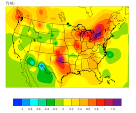
WRFDA 4D-Var can assimilate NCEP Stage IV radar and gauge precipitation data. NCEP Stage IV archived data are available on the NCAR CODIAC web page at: http://data.eol.ucar.edu/codiac/dss/id=21.093 (for more information, please see the NCEP Stage IV Q&A Web page at http://www.emc.ncep.noaa.gov/mmb/ylin/pcpanl/QandA/). The original precipitation data are at 4-km resolution on a polar-stereographic grid. Hourly, 6-hourly and 24-hourly analyses are available. The following image shows the accumulated 6-h precipitation for the tutorial case.

2008020518

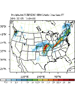
It should be mentioned that the NCEP Stage IV archived data is in GRIB1 format and it cannot be ingested into the WRFDA directly. A tool “precip_converter” is provided to reformat GRIB1 observations into the WRFDA-readable ASCII format. It can be downloaded from the WRFDA users page at http://www2.mmm.ucar.edu/wrf/users/wrfda/download/precip_converter.tar.gz. The NCEP GRIB libraries, w3 and g2 are required to compile the precip_converter utility. These libraries are available for download from NCEP at http://www.nco.ncep.noaa.gov/pmb/codes/GRIB2/. The output file to the precip_converter utility is named in the format ob.rain.yyyymmddhh.xxh; The 'yyyymmddhh' in the file name is the ending hour of the accumulation period, and 'xx' (=01,06 or 24) is the accumulating time period.

For users wishing to use their own observations instead of NCEP Stage IV, it is the user’s responsibility to write a Fortran main program and call subroutine writerainobs (in write_rainobs.f90) to generate their own precipitation data. For more information please refer to the README file in the precip_converter directory.

b. Running WRFDA 4D-Var with precipitation observations

WRFDA 4D-Var is able to assimilate hourly, 3-hourly and 6-hourly precipitation data. According to experiments and related scientific papers, 6-hour precipitation accumulations are the ideal observations to be assimilated, as this leads to better results than directly assimilating hourly data.

The tutorial example is for assimilating 6-hour accumulated precipitation. In your working directory, link all the necessary files as follows,

> ln -fs $WRFDA_DIR/var/da/da_wrfvar.exe .

> ln -fs $DAT_DIR/rc/2008020512/wrfinput_d01 .

> ln -fs $DAT_DIR/rc/2008020512/wrfbdy_d01 .

> ln -fs $DAT_DIR/rc/2008020518/wrfinput_d01 fg02 (only necessary for var4d_lbc=true)

> ln -fs wrfinput_d01 fg

> ln -fs $DAT_DIR/be/be.dat .

> ln -fs $WRFDA_DIR/run/LANDUSE.TBL .

> ln -fs $WRFDA_DIR/run/RRTM_DATA_DBL ./RRTM_DATA

> ln -fs $DAT_DIR/ob/2008020518/ob.rain.2008020518.06h ob07.rain

Note: The reason why the observation ob.rain.2008020518.06h is linked as ob07.rain will be explained in section d.

Edit namelist.input (you can start with the same namelist as for the 4dvar tutorial case) and pay special attention to &wrfvar1 and &wrfvar4 for precipitation-related options.

&wrfvar1

var4d=true,

var4d_lbc=true,

var4d_bin=3600,

var4d_bin_rain=21600,

……
/

……

&wrfvar4

use_rainobs=true,

thin_rainobs=true,

thin_mesh_conv=28*20.,

Then, run 4D-Var in serial or parallel mode,

>./da_wrfvar.exe >& wrfda.log

c. Namelist variables to control precipitation assimilation

var4d_bin_rain

Precipitation observation sub-window length for 4D-Var. It does not need to be consistent with var4d_bin.

thin_rainobs

Logical, TRUE will perform thinning on precipitation data.

thin_mesh_conv

Specify thinning mesh size (in km)

d. Properly linking observation files

In section b, ob.rain.2008020518.06h is linked as ob07.rain. The number 07 is assigned according to the following rule:

x=i*(var4d_bin_rain/var4d_bin)+1,

Here, i is the sequence number of the observation.

for x<10, the observation file should be renamed as ob0x.rain;

for x>=10, it should be renamed as obx.rain

In the example above, 6-hour accumulated precipitation data is assimilated in 6-hour time window. In the namelist, values should be set at var4d_bin=3600 and var4d_bin_rain=21600, and there is one observation file (i.e., i=1) in the time window, Thus the value of x is 7. The file ob.rain.2008020518.06h should be renamed as ob07.rain.

Let us take another example for how to rename observation files for 3-hourly precipitation data in 6-hour time window. The sample namelist is as follows,

&wrfvar1

var4d=true,

var4d_lbc=true,

var4d_bin=3600,

var4d_bin_rain=10800,

……
/

There are two observation files, ob.rain.2008020515.03h and ob.rain.2008020518.03h. For the first file (i=1) ob.rain.2008020515.03h, it should be renamed as ob04.rain,and the second file (i=2) renamed as ob07.rain.

Updating WRF Boundary Conditions

a. Lateral boundary conditions

When using WRFDA output to run a WRF forecast, it is essential that you update the WRF lateral boundary conditions (contained in the file wrfbdy_01, created by real.exe) to match your new analysis. Domain-1 (wrfbdy_d01) must be updated to be consistent with the new WRFDA initial condition (analysis). This is absolutely essential. For nested domains, domain-2, domain-3, etc., the lateral boundary conditions are provided by their parent domains, so no lateral boundary update is needed for these domains. The update procedure is performed by the WRFDA utility called da_update_bc.exe, and after compilation can be found in $WRFDA_DIR/var/build.

da_update_bc.exe requires three input files: the WRFDA analysis (wrfvar_output), the wrfbdy file from real.exe, and a namelist file: parame.in. To run da_update_bc.exe to update lateral boundary conditions, follow the steps below:

> cd $WRFDA_DIR/var/test/update_bc

> cp –p $DAT_DIR/rc/2008020512/wrfbdy_d01 .

(IMPORTANT: make a copy of wrfbdy_d01, as the wrf_bdy_file will be overwritten by da_update_bc.exe)

> vi parame.in

&control_param

da_file = '../tutorial/wrfvar_output'

wrf_bdy_file = './wrfbdy_d01'

domain_id = 1

debug = .true.

update_lateral_bdy = .true.

update_low_bdy = .false.

update_lsm = .false.

iswater = 16

var4d_lbc = .false.

> ln –sf $WRFDA_DIR/var/da/da_update_bc.exe .

> ./da_update_bc.exe

At this stage, you should have the files wrfvar_output and wrfbdy_d01 in your WRFDA working directory. They are the WRFDA updated initial and boundary condition files for any subsequent WRF model runs. To use, link a copy of wrfvar_output and wrfbdy_d01 to wrfinput_d01 and wrfbdy_d01, respectively, in your WRF working directory.

You should also see two additional output files: fort.11 and fort.12. These contain information about the changes made to wrfbdy_01.

b. Cycling with WRF and WRFDA (warm-start)

In cycling mode (warm-start), the lower boundary in the first guess file also needs to be updated based on the information from the wrfinput file, generated by WPS/real.exe at analysis time. If in cycling mode (especially if you are doing radiance data assimilation and there are SEA ICE or SNOW in your domain), it is recommended that before you run WRFDA, you run da_update_bc.exe with the following namelist options:

da_file = './fg'

wrf_input = './wrfinput_d01'

update_lateral_bdy = .false.

update_low_bdy = .true.

iswater = 16

Note: “iswater” (water point index) is 16 for USGS LANDUSE and 17 for MODIS LANDUSE.

This creates a lower-boundary updated first guess (da_file will be overwritten by da_update_bc with updated lower boundary conditions from wrf_input). Then, after WRFDA has finished, run da_update_bc.exe again with the following namelist options:

da_file = './wrfvar_output'

wrf_bdy_file = './wrfbdy_d01'

update_lateral_bdy = .true.

update_low_bdy = .false.

This updates the lateral boundary conditions (wrf_bdy_file will be overwritten by da_update_bc with lateral boundary conditions from da_file).

As mentioned previously, lateral boundary conditions for child domains (wrfinput_02, wrfinput_03, etc.) come from the respective parent domains, so update_bc is not necessary after running WRFDA. However, in a cycling procedure, the lower boundaries in each of the nested domains’ WRFDA analysis files still need to be updated. In these cases, you must set the namelist variable, domain_id > 1 (default is 1 for domain-1) and provide the appropriate wrfinput file (wrf_input = './wrfinput_d02' for domain 2, for instance).

c. WRFDA 4DVAR with lateral boundary conditions as control variables

If you activate the var4d_lbc option in a WRF 4D-Var run, in addition to the above-mentioned files you will also need the ana02 file from the WRFDA working directory. In parame.in, set var4d_lbc to TRUE and use “da_file_02” to point to the location of the ana02 file.

da_file_02 = './ana02'

var4d_lbc = .true.

Background Error and running GEN_BE

Users have four choices to define the background error covariance (BE). We call them CV3, CV5, CV6, and CV7. Each of these has different properties, which are outlined in the table below:

CV option	Data source	Control variables	cv_options =
CV3	Provided be.dat file	ψ, χ_u, T_u, q, P_s,u	3
CV5	GEN_BE	ψ, χ_u, T_u, RH_s, P_s,u	5
CV6	GEN_BE	ψ, χ_u, T_u, RH_s,u, P_s,u	6
CV7	GEN_BE	u, v, T, RH_s, P_s	7

With CV3, the control variables are in physical space while with CV5, CV6, and CV7, the control variables are in eigenvector space. The major difference between these two kinds of BE is the vertical covariance; CV3 uses the vertical recursive filter to model the vertical covariance but the others use an empirical orthogonal function (EOF) to represent the vertical covariance. The recursive filters to model the horizontal covariance are also different with these BEs. We have not conducted the systematic comparison of the analyses based on these BEs. However, CV3 (a BE file provided with our WRFDA system) is a global BE and can be used for any regional domain, while CV5, CV6, and CV7 BE’s are domain-dependent, and so should be generated based on forecast or ensemble data from the same domain.

As summarized in the above table, CV5, CV6, and CV7 differ in the control variables they use. CV5 utilizes streamfunction (ψ), unbalanced velocity potential (χ_u), unbalanced temperature (T_u), pseudo relative humidity (RH_s), and unbalanced surface pressure (P_s,u). The pseudo relative humidity is defined as Q/Q_b,s, where Q_b,sis the saturated specific humidity from the background field. For CV6 the moisture control variable is the unbalanced portion of the pseudo relative humidity (RH_s,u). Additionally, CV6 introduces six additional correlation coefficients in the definition of the balanced part of analysis control variables. See the section GEN_BE for CV6 for more details on this option. Finally, CV7 uses a different set of control variables: u, v, temperature, pseudo relative humidity (RH_s), and surface pressure (P_s).

Generic BE option: CV3

CV3 is the NCEP background error covariance. It is estimated in grid space by what has become known as the NMC method (Parrish and Derber 1992) . The statistics are estimated with the differences of 24 and 48-hour GFS forecasts with T170 resolution, valid at the same time for 357 cases, distributed over a period of one year. Both the amplitudes and the scales of the background error have to be tuned to represent the forecast error in the estimated fields. The statistics that project multivariate relations among variables are also derived from the NMC method.

The variance of each variable, and the variance of its second derivative, are used to estimate its horizontal scales. For example, the horizontal scales of the stream function can be estimated from the variance of the vorticity and stream function.

The vertical scales are estimated with the vertical correlation of each variable. A table is built to cover the range of vertical scales for the variables. The table is then used to find the scales in vertical grid units. The filter profile and the vertical correlation are fitted locally. The scale of the best fit from the table is assigned as the scale of the variable at that vertical level for each latitude. Note that the vertical scales are locally defined so that the negative correlation further away, in the vertical direction, is not included.

Theoretically, CV3 BE is a generic background error statistics file which can be used for any case. It is quite straightforward to use CV3 in your own case. To use the CV3 BE file in your case, set cv_options=3 in &wrfvar7 in namelist.input in your working directory, and use the be.dat is located in WRFDA/var/run/be.dat.cv3.

Modifying CV3 length scales and variance

Because CV3 is a generic background error option, it is necessary to tune the default background error scale length and variance values for each experiment. These can be controlled at run time with a series of namelist variables described below.

The scaling factors for CV3 are stored as an array of values for each individual control

variable:

as1: stream function

as2: unbalanced velocity potential

as3: unbalanced temperature

as4: pseudo relative humidity

as5: unbalanced surface pressure

These variables are all 3-element vectors. The first element is the variance scaling factor. The second is the horizontal length scale factor. The third is the vertical length scale factor. So setting the default values in your namelist would look like this:

&wrfvar7

cv_options = 3,

as1 = 0.25, 1.00, 1.50,

as2 = 0.25, 1.00, 1.50,

as3 = 0.25, 1.00, 1.50,

as4 = 0.25, 1.00, 1.50,

as5 = 0.25, 1.00, 1.50,

The first column is the variance, the second is the horizontal length scale factor, and the third is the vertical length scale factor.

For multiple outer loops, the next 3 elements of each vector must be filled in. So for 2 outer loops (max_ext_its=2), to use the default values, the namelist should look like this:

&wrfvar7

cv_options = 3,

as1 = 0.25, 1.00, 1.50, 0.25, 1.00, 1.50,

as2 = 0.25, 1.00, 1.50, 0.25, 1.00, 1.50,

as3 = 0.25, 1.00, 1.50, 0.25, 1.00, 1.50,

as4 = 0.25, 1.00, 1.50, 0.25, 1.00, 1.50,

as5 = 0.25, 1.00, 1.50, 0.25, 1.00, 1.50,

Again, the first column is the variance, the second is the horizontal length scale factor, and the third is the vertical length scale factor for the first outer loop. The fourth column is the variance, the fifth is the horizontal length scale factor, and the sixth is the vertical length scale factor for the second outer loop.

Continue in this manner for more outer loops. The values listed above are the default values, but can be adjusted for each individual experiment.

Domain-specific background error options: Running GEN_BE

To use CV5, CV6 or CV7 background error covariance, it is necessary to generate your domain-specific background error statistics with the gen_be utility. The default CV3 background error statistics file, supplied with the WRFDA source code, can NOT be used with these control variable options.

The main source code for the various gen_be stages can be found in WRFDA/var/gen_be. The executables of gen_be should have been created when you compiled the WRFDA code (as described earlier). The scripts to run these codes are in WRFDA/var/scripts/gen_be.

The input data for gen_be are WRF forecasts, which are used to generate model perturbations, used as a proxy for estimates of forecast error. For the NMC-method, the model perturbations are differences between forecasts (e.g. T+24 minus T+12 is typical for regional applications, T+48 minus T+24 for global) valid at the same time. Climatological estimates of background error may then be obtained by averaging these forecast differences over a period of time (e.g. one month). Given input from an ensemble prediction system (EPS), the inputs are the ensemble forecasts, and the model perturbations created are the transformed ensemble perturbations. The gen_be code has been designed to work with either forecast difference or ensemble-based perturbations. The former is illustrated in this tutorial example.

It is important to include forecast differences, from at least 00Z and 12Z through the period, to remove the diurnal cycle (i.e. do not run gen_be using model perturbations valid for a single time each day).

The inputs to gen_be are netCDF WRF forecast output ("wrfout") files at specified forecast ranges. To avoid unnecessary large single data files, it is assumed that all forecast ranges are output to separate files. For example, if we wish to calculate BE statistics using the NMC-method with (T+24)-(T+12) forecast differences (default for regional) then by setting the WRF namelist.input options history_interval=720, and frames_per_outfile=1 we get the necessary output datasets. Then the forecast output files should be arranged as follows: directory name is the forecast initial time, time info in the file name is the forecast valid time. 2008020512/wrfout_d01_2008-02-06_00:00:00 means a 12-hour forecast valid at 2008020600, initialized at 2008020512.

Example dataset for a test case (90 x 60 x 41 gridpoints) can be downloaded from http://www2.mmm.ucar.edu/wrf/users/wrfda/download/testdata.html. Untar the gen_be_forecasts_20080205.tar.gz file. You will have:

>ls $FC_DIR

-rw-r--r-- 1 users 11556492 2008020512/wrfout_d01_2008-02-06_00:00:00

-rw-r--r-- 1 users 11556492 2008020512/wrfout_d01_2008-02-06_12:00:00

-rw-r--r-- 1 users 11556492 2008020600/wrfout_d01_2008-02-06_12:00:00

-rw-r--r-- 1 users 11556492 2008020600/wrfout_d01_2008-02-07_00:00:00

-rw-r--r-- 1 users 11556492 2008020612/wrfout_d01_2008-02-07_00:00:00

-rw-r--r-- 1 users 11556492 2008020612/wrfout_d01_2008-02-07_12:00:00

In the above example, only 1 day (12Z 05 Feb to 12Z 06 Feb. 2008) of forecasts, every 12 hours is supplied to gen_be_wrapper to estimate forecast error covariance. It is only for demonstration. The minimum number of forecasts required depends on the application, number of grid points, etc. Month-long (or longer) datasets are typical for the NMC-method. Generally, at least a 1-month dataset should be used.

Under WRFDA/var/scripts/gen_be, gen_be_wrapper.ksh is used to generate the BE data. The following variables need to be set to fit your case:

export WRFVAR_DIR=/glade/p/work/wrfhelp/PRE_COMPILED_CODE/WRFDA

export NL_CV_OPTIONS=5 # 5 for CV5, 7 for CV7

export START_DATE=2008020612 # the first perturbation valid date

export END_DATE=2008020700 # the last perturbation valid date

export NUM_LEVELS=40 # e_vert - 1

export BIN_TYPE=5 # How data is binned for calculating statistics

export FC_DIR=/glade/p/work/wrfhelp/WRFDA_DATA/fc # where wrf forecasts are

export RUN_DIR=`pwd`/gen_be # Where GEN_BE will run and output files

Note: The START_DATE and END_DATE are perturbation valid dates. As shown in the forecast list above, when you have 24-hour and 12-hour forecasts initialized at 2008020512, through 2008020612, the first and final forecast difference valid dates are 2008020612 and 2008020700, respectively.

Note: The forecast dataset should be located in $FC_DIR. Then type:

> gen_be_wrapper.ksh

Once the gen_be_wrapper.ksh run is completed, the be.dat can be found under the $RUN_DIR directory.

To get a clear idea about what is included in be.dat, the script gen_be_plot_wrapper.ksh may be used. This plots various data in be.dat; for example:

Note: Make sure that you remove the first two lines (header) in cost_fn and grad_fn before you plot. You also need to specify the directory name for these two files.

gts_omb_oma_01: It contains (in ASCII format) information on all of the observations used by the WRFDA run. Each observation has its observed value, quality flag, observation error, observation minus background (OMB), and observation minus analysis (OMA). This information is very useful for both analysis and forecast verification purposes.

namelist.input: This is the WRFDA input namelist file, which contains all the user-defined non-default options. Any namelist-defined options that do not appear in this file should have their names checked against the values in $WRFDA_DIR/Registry/registry.var.

namelist.output.da: A list of all the namelist options used. If an option was not specified in namelist.input, the default listed in the registry value will be used.

rsl*: Files containing information for standard WRFDA output from individual processors when multiple processors are used. It contains a host of information on a number of observations, minimization, timings, etc. Additional diagnostics may be printed in these files by including various “print” WRFDA namelist options. To learn more about these additional “print” options, search for the “print_” string in $WRFDA_DIR/Registry/registry.var.

statistics: Text file containing OMB (OI) and OMA (OA) statistics (minimum, maximum, mean and standard deviation) for each observation type and variable. This information is very useful in diagnosing how WRFDA has used different components of the observing system. Also contained are the analysis minus background (A-B) statistics, i.e. statistics of the analysis increments for each model variable at each model level. This information is very useful in checking the range of analysis increment values found in the analysis, and where they are in the WRF-model grid space.

The WRFDA analysis file is wrfvar_output. It is in WRF (netCDF) format. It will become the input file wrfinput_d01 of any subsequent WRF run after lateral boundary and/or lower boundary conditions are updated by another WRFDA utility (See the section Updating WRF boundary conditions).

An NCL script, $TOOLS_DIR/var/graphics/ncl/WRF-Var_plot.ncl, is provided in the tools package for plotting. You need to specify the analysis_file name, its full path, etc. Please see the in-line comments in the script for details.

As an example, if you are aiming to display the U-component of the analysis at level 18, use the script WRF-Var_plot.ncl, and make sure the following pieces of codes are uncommented:

var = "U"

fg = first_guess->U

an = analysis->U

plot_data = an

When you execute the following command from $WRFDA_DIR/var/graphics/ncl.

> ncl WRF-Var_plot.ncl

The plot should look like:

You may change the variable name, level, etc. in this script to display the variable of your choice at the desired eta level.

Take time to look through the text output files to ensure you understand how WRFDA works. For example:

How closely has WRFDA fit individual observation types? Look at the statistics file to compare the O-B and O-A statistics.

How big are the analysis increments? Again, look in the statistics file to see minimum/maximum values of A-B for each variable at various levels. It will give you a feel for the impact of the input observation data you assimilated via WRFDA by modifying the input analysis first guess.

How long did WRFDA take to converge? Does it really converge? You will get the answers of all these questions by looking into the rsl.* -files, as it indicates the number of iterations taken by WRFDA to converge. If this is the same as the maximum number of iterations specified in the namelist (NTMAX), or its default value (=200) set in $WRFDA_DIR/Registry/registry.var, then it means that the analysis solution did not converge. If this is the case, you may need to increase the value of “NTMAX” and rerun your case to ensure that the convergence is achieved. On the other hand, a normal WRFDA run should usually converge within 100 iterations. If it still doesn’t converge in 200 iterations, that means there may be a problem in the observations or first guess.

A good way to visualize the impact of assimilation of observations is to plot the analysis increments (i.e. analysis minus the first guess difference). Many different graphics packages (e.g. RIP4, NCL, GRADS etc) can do this.

You need to modify this script to fix the full path for first_guess and analysis files. You may also use it to modify the display level by setting kl and the name of the variable to display by setting var. Further details are given in this script.

If you are aiming to display the increment of potential temperature at level 18, after modifying $WRFDA_DIR/var/graphics/ncl/WRF-Var_plot.ncl, make sure the following pieces of code are uncommented:

var = "T"

fg = first_guess->T ;Theta- 300

an = analysis->T ;Theta- 300

plot_data = an - fg

When you execute the following command from WRFDA_DIR/var/graphics/ncl.

> ncl WRF-Var_plot.ncl

The plot created will look as follows:

Note: Larger analysis increments indicate a larger data impact in the corresponding region of the domain.

Generating ensembles with RANDOMCV

In addition to the variational methods previously mentioned, the WRFDA system supports both ensemble and hybrid ensemble/variational assimilation methods. To utilize these methods, having an ensemble of forecasts is necessary. WRFDA has a built-in method for generating ensemble initial conditions known as RANDOMCV. RANDOMCV works by adding random noise to the analysis in control variable space.

a. Running WRFDA for RANDOMCV

RANDOMCV is a capability of the main WRFDA executable, so you will run it by setting the following variables in namelist.input and then running da_wrfvar.exe as you would with any data assimilation run:

&wrfvar5

put_rand_seed true: enter your own seed numbers to generate random background perturbations. The advantage of this setting is that the same seed numbers will always produce the same perturbation
false: (default behavior) perturbations will be generated “randomly” and give new perturbations each time

&wrfvar11

seed_array1 First integer for seeding the random function (default: 1)

seed_array2 Second integer for seeding the random function (default: 1) It is not necessary to change both seeds to get different perturbations

&wrfvar17

analysis_type Set this to ‘RANDOMCV’ to use the RANDOMCV capability

When setting your own random seeds, a common good practice is to set the first seed as the experiment date/time in integer form, and the second seed as the ensemble member number. The seeds should not be set to zero.

Because the perturbations are made in control variable space, the general pattern of perturbations will depend on your background error. You should be able to use any background error option with RANDOMCV (CV3, CV5, CV6, or CV7). Additionally, this means you can control their magnitude and lengthscales by modifying the background error variance and length scaling variables respectively:

For CV5, CV6, or CV7

&wrfvar7

var_scaling1 = 0.25, # reduce psi perturbation magnitude by 75%

var_scaling2 = 0.25, # reduce chi_u perturbation magnitude by 75%

var_scaling3 = 0.0, # reduce T perturbation by 100% (there will be no T perturbation!)

var_scaling4 = 2.0, # increase q perturbation by 100%

var_scaling5 = 1.0, # Keep Ps perturbation magnitude the same

var_scaling1 = 0.5, # reduce psi perturbation length scale by 50%

var_scaling2 = 0.5, # reduce chi_u perturbation length scale by 50%

var_scaling3 = 1.0, # Keep T perturbation length scale the same

var_scaling4 = 2.0, # increase q perturbation length scale by 100%

var_scaling5 = 1.5, # increase Ps perturbation length scale by 50%

For CV3, see the section “Modifying CV3 length scales and variance”.

Hybrid Data Assimilation in WRFDA

The WRFDA system also includes a hybrid data assimilation technique, which is based on the existing 3D-Var. The difference between hybrid and 3D-Var schemes is that 3D-Var relies solely on a static covariance model to specify the background errors, while the hybrid system uses a combination of 3D-Var static error covariances and ensemble-estimated error covariances to incorporate a flow-dependent estimate of the background error statistics. The following section will give a brief introduction of some aspects of using the hybrid system. Please refer to these papers for a detailed description of the methodology used in the WRFDA hybrid system:

Xuguang Wang, Dale M. Barker, Chris Snyder, and Thomas M. Hamill, 2008: A hybrid ETKF–3DVAR data assimilation scheme for the WRF model. Part I: Observing system simulation experiment. Mon. Wea. Rev., 136, 5116–5131.

Xuguang Wang, Dale M. Barker, Chris Snyder, and Thomas M. Hamill, 2008: A Hybrid ETKF–3DVAR Data Assimilation Scheme for the WRF Model. Part II: Real Observation Experiments. Mon. Wea. Rev., 136, 5132–5147.

b. Source code

Four executables are used in the hybrid system. If you have successfully compiled the WRFDA system, the following executables will exist in the WRFDA/var/build directory:

WRFDA/var/build/gen_be_ensmean.exe

WRFDA/var/build/gen_be_ep2.exe

WRFDA/var/build/da_wrfvar.exe

WRFDA/var/build/gen_be_vertloc.exe

gen_be_ensmean.exe is used to calculate the ensemble mean, while gen_be_ep2.exe is used to calculate the ensemble perturbations. gen_be_vertloc.exe is used for vertical localization. As with 3D-Var/4D-Var, da_wrfvar.exe is the main WRFDA program. However, in this case, da_wrfvar.exe will run in hybrid mode.

c. Running the hybrid system

The procedure is the same as running 3D-Var/4D-Var, with the exception of some extra input files and namelist settings. The basic input files for WRFDA are LANDUSE.TBL, ob.ascii or ob.bufr (depending on which observation format you use), and be.dat (static background errors). Additional input files required by the hybrid are a single ensemble mean file (used as the fg for the hybrid application) and a set of ensemble perturbation files (used to represent flow-dependent background errors).

A set of initial ensemble members must be prepared before the hybrid application can be started. The ensemble can be obtained from other ensemble model outputs, or you can generate them yourself. This can be done, for example, adding random noise to the initial conditions at a previous time and integrating each member to the desired time. A tutorial case with a test ensemble can be found at http://www2.mmm.ucar.edu/wrf/users/wrfda/download/V38/wrfda_hybrid_etkf_testdata.tar.gz. In this example, the ensemble forecasts were initialized at 2015102612 and valid 2015102712. A hybrid analysis at 2015102712 will be performed using the ensemble valid 2015102712 as input. Once you have the initial ensemble, the ensemble mean and perturbations can be calculated following the steps below:

1) Set an environment variable for your working directory and your data directory

> setenv WORK_DIR your_hybrid_path
> setenv DAT_DIR your_data_path
> cd $WORK_DIR

2) Calculate the ensemble mean

a) From your working directory, copy or link the ensemble forecasts to your working directory. The ensemble members are identified by three-digit numbers following the valid time.

> ln –sf $DAT_DIR/Hybrid/fc/2015102612/wrfout_d01_2015-10-27_12:00:00.e* .

b) Provide two template files (ensemble mean and variance files) in your working directory. These files will be overwritten with the ensemble mean and variance as discussed below.

> cp $DAT_DIR/Hybrid/fc/2015102612/wrfout_d01_2015-10-27_12:00:00.e001 ./wrfout_d01_2015-10-27_12:00:00.mean
> cp $DAT_DIR/Hybrid/fc/2015102612/wrfout_d01_2015-10-27_12:00:00.e001 ./wrfout_d01_2015-10-27_12:00:00.vari

c) Copy gen_be_ensmean_nl.nl (cp $DAT_DIR/Hybrid/gen_be_ensmean_nl.nl .) You will need to set the information in this script as follows:

&gen_be_ensmean_nl
directory = '.'
filename = 'wrfout_d01_2015-10-27_12:00:00'
num_members = 10
nv = 7
cv = 'U', 'V', 'W', 'PH', 'T', 'MU', 'QVAPOR'
/

where directory is the folder containing the ensemble members and template files, filename is the name of the files before their suffixes (e.g., .mean, .vari, etc), num_members is the number of ensemble members you are using, nv is the number of variables, and cv is the name of variables used in the hybrid system. Be sure nv and cv are consistent!

d) Link gen_be_ensmean.exe to your working directory and run it.

> ln –sf $WRFDA_DIR/var/build/gen_be_ensmean.exe .
> ./gen_be_ensmean.exe

Check the output files. wrfout_d01_2015-10-27_12:00:00.mean is the ensemble mean; wrfout_d01_2015-10-27_12:00:00.vari is the ensemble variance

3) Calculate ensemble perturbations

a) Create a sub-directory in which you will be working to create ensemble perturbations.

> mkdir –p ./ep
> cd ./ep

b) Run gen_be_ep2.exe. The executable requires four command-line arguments (DATE, NUM_MEMBER, DIRECTORY, and FILENAME) as shown below for the tutorial example:

> ln –sf $WRFDA_DIR/var/build/gen_be_ep2.exe .
> ./gen_be_ep2.exe 2015102712 10 . ../wrfout_d01_2015-10-27_12:00:00

c) Check the output files. A list of binary files should now exist. Among them, tmp.e* are temporary scratch files that can be removed.

4) Back in the working directory, create the input file for vertical localization. This program requires one command-line argument: the number of vertical levels of the model configuration (same value as e_vert in the namelist; for the tutorial example, this should be 42).

> cd $WORK_DIR

> ln –sf $WRFDA_DIR/var/build/gen_be_vertloc.exe .

> ./gen_be_vertloc.exe 42

The output is ./be.vertloc.dat in your working directory.

5) Run WRFDA in hybrid mode

a) In your hybrid working directory, link all the necessary files and directories as follows:

> ln -fs ./ep/* .
> ln -fs ./wrfout_d01_2015-10-27_12:00:00.mean ./fg (first guess is the ensemble mean for this test case)
> ln -fs $WRFDA_DIR/run/LANDUSE.TBL .
> ln -fs $DAT_DIR/Hybrid/ob/2015102712/ob.ascii ./ob.ascii
> ln -fs $DAT_DIR/Hybrid/be/be.dat ./be.dat
> ln –fs $WRFDA_DIR/var/build/da_wrfvar.exe .
> cp $DAT_DIR/Hybrid/namelist.input .

b) Edit namelist.input, paying special attention to the following hybrid-related settings:

&wrfvar7
je_factor = 2.0
/
&wrfvar16
ensdim_alpha = 10
alphacv_method = 2
alpha_corr_type=3
alpha_corr_scale = 500.0
alpha_std_dev=1.000
alpha_vertloc = .true.
/

c) Finally, execute the WRFDA file, running in hybrid mode

> ./da_wrfvar.exe >& wrfda.log

Check the output files; the output file lists are the same as when you run WRF 3D-Var.

d. Hybrid namelist options

je_factor

ensemble covariance weighting factor. This factor controls the weighting component of ensemble and static covariances. The corresponding jb_factor = je_factor/(je_factor - 1).

ensdim_alpha

the number of ensemble members. Hybrid mode is activated when ensdim_alpha is larger than zero

alphacv_method

1=perturbations in control variable space (“psi”,”chi_u”,”t_u”,”rh”,”ps_u”); 2=perturbations in model space (“u”,”v”,”t”,”q”,”ps”). Option 2 is extensively tested and recommended to use.

alpha_corr_type

correlation function. 1=Exponential; 2=SOAR; 3=Gaussian.

alpha_corr_scale

hybrid covariance localization scale in km unit. Default value is 200.

alpha_std_dev

alpha standard deviation. Default value is 1.0

alpha_vertloc

for vertical localization. .true.=use vertical localization; .false.=no vertical localization

ETKF Data Assimilation

The WRFDA system also includes a ETKF assimilation technique. The ETKF system updates the ensemble perturbations. Please refer to Bishop et al. (2001) and Wang et al. (2003) for a detailed description of the methodology. The following section will give a brief introduction of some aspects of using the ETKF system.

a. Source Code

Three executables are used in the ETKF system. If you have successfully compiled the WRFDA system, you will see the following:

WRFDA/var/build/gen_be_etkf.exe

WRFDA/var/build/gen_be_addmean.exe

WRFDA/var/build/da_wrfvar.exe

The file gen_be_etkf.exe is used to update the ensemble perturbations, while gen_be_addmean.exe is used to combine the ensemble mean and the ensemble perturbations. As with 3D-Var/4D-Var, da_wrfvar.exe is the main WRFDA program. However, in this case, da_wrfvar.exe will create filtered observations and prepare formatted omb files for ETKF.

b. Running the ETKF System

The first procedure is to update the ensemble perturbations. A set of initial ensemble members must be prepared before the ETKF application can be started. The ensemble can be obtained from a previous ensemble forecast. A tutorial case with a test ensemble can be found at http://www2.mmm.ucar.edu/wrf/users/wrfda/download/V38/wrfda_hybrid_etkf_testdata.tar.gz. In this example, the ensemble forecasts were initialized at 2015102612 and valid 2015102712. ETKF will be performed using the ensemble valid 2015102712 as input. Once you have the initial ensemble, the ensemble perturbations can be updated by following the steps below:

1) Set environment variables for convenience

> setenv WORK_DIR_ETKF your_etkf_path

> setenv DAT_DIR your_data_path

> setenv WRFDA_DIR your_WRFDA_path

> cd $WORK_DIR_ETKF

2) Prepare the filtered observations

a) In your ETKF working directory, make a subdirectory to prepare the filtered

observations and link all the necessary files and directories as follows:

> mkdir obs_filter

> cd obs_filter

> ln -fs $DAT_DIR/Hybrid/fc/2015102612/wrfout_d01_2015-10-27_12:00:00.mean ./fg (first guess is the ensemble mean)

> ln -fs $WRFDA_DIR/run/LANDUSE.TBL .

> ln -fs $DAT_DIR/Hybrid/ob/2015102712/ob.ascii ./ob.ascii

> ln -fs $DAT_DIR/Hybrid/be/be.dat ./be.dat

> ln -fs $WRFDA_DIR/var/build/da_wrfvar.exe .

> cp $DAT_DIR/ETKF/namelist.input .

b) Edit namelist.input, paying special attention to the following 'QC-OBS'-related settings:

&wrfvar17

analysis_type = 'QC-OBS',

c) Execute the WRFDA file, running in QC-OBS mode

> ./da_wrfvar.exe >& wrfda.log

Check the output files; you should see a 'filtered_obs_01' file which contains the filtered observations.

3) Prepare omb files for ETKF

a) In your ETKF working directory, make a subdirectory to prepare the omb files for each ensemble member and link all the necessary files and directories as follows:

> cd $WORK_DIR_ETKF

> mkdir -p omb/working.e001

> cd omb/working.e001

> ln -fs $DAT_DIR/Hybrid/fc/2015102612/wrfout_d01_2015-10-27_12:00:00.e001 ./fg (first guess is the ensemble member)

> ln -fs $WRFDA_DIR/run/LANDUSE.TBL .

> ln -fs $WORK_DIR_ETKF/obs_filter/filtered_obs_01 ./ob.ascii

> ln -fs $DAT_DIR/Hybrid/be/be.dat ./be.dat

> ln -fs $WRFDA_DIR/var/build/da_wrfvar.exe .

> cp $DAT_DIR/ETKF/namelist.input .

b) Edit namelist.input, paying special attention to the following 'VERIFY'-related settings:

&wrfvar17

analysis_type = 'VERIFY',

c) Execute the WRFDA file, running in VERIFY mode

> ./da_wrfvar.exe >& wrfda.log

Check the output files. The output files are the same as when you run WRF 3D-Var (except wrfvar_output will NOT be created), and the 'ob.etkf.0*' files are omb files.

d) Combine the ob.etkf.0* files and add the observation number in the head of ob.etkf.e0*

> cat ob.etkf.0* > ob.all

> wc -l ob.all > ob.etkf.e001

> cat ob.all >> ob.etkf.e001

e) Likewise, prepare ob.etkf.e0* files for other ensemble members

4) Run ETKF

a) Copy or link the ensemble mean and forecasts and ob.etkf.e0* files to your working directory and make a parameter directory to save the parameter files.

> cd $WORK_DIR_ETKF

> setenv PAR_DIR_ETKF $WORK_DIR_ETKF/param

> mkdir $PAR_DIR_ETKF

> ln -sf $DAT_DIR/Hybrid/fc/2015102612/wrfout_d01_2015-10-27_12:00:00.mean ./etkf_input

> ln -sf $DAT_DIR/Hybrid/fc/2015102612/wrfout_d01_2015-10-27_12:00:00.e001 ./etkf_input.e001

...

> ln -sf $DAT_DIR/Hybrid/fc/2015102712/wrfout_d01_2015-10-27_12:00:00.e010 ./etkf_input.e010

> ln -sf omb/working.e001/ob.etkf.e001 .

...

> ln -sf omb/working.e010/ob.etkf.e010 .

b) Provide template files. These files will be overwritten with the ensemble perturbations.

> cp $DAT_DIR/Hybrid/fc/2015102612/wrfout_d01_2015-10-27_12:00:00.e001 ./etkf_output.e001

...

> cp $DAT_DIR/Hybrid/fc/2015102612/wrfout_d01_2015-10-27_12:00:00.e010 ./etkf_output.e010

c) Copy gen_be_etkf_nl.nl (cp $DAT_DIR/ETKF/gen_be_etkf_nl.nl .)

You will need to set the information in this script as follows:

&gen_be_etkf_nl

num_members = 10,

nv = 7,

cv = 'U', 'V', 'W', 'PH', 'T', 'QVAPOR', 'MU',

naccumt1 = 20,

naccumt2 = 20,

nstartaccum1 = 1,

nstartaccum2 = 1,

nout = 1,

tainflatinput = 1,

rhoinput = 1,

infl_fac_file = '$PAR_DIR_ETKF/inflation_factor.dat',

infl_let_file = '$PAR_DIR_ETKF/inflation_letkf.dat',

eigen_val_file = '$PAR_DIR_ETKF/eigen_value.dat',

inno2_val_file = '$PAR_DIR_ETKF/innovation_value.dat',

proj2_val_file = '$PAR_DIR_ETKF/projection_value.dat',

infl_fac_TRNK = .false.,

infl_fac_WG03 = .false.,

infl_fac_WG07 = .true.,

infl_fac_BOWL = .false.,

letkf_flg=.false.,

rand_filt = .false.,

rnd_seed = 2015102712,

rnd_nobs = 5000

etkf_erro_max = 20.

etkf_erro_min = .00001

etkf_inno_max = 20.

etkf_inno_min = .00001

etkf_erro_flg = .true.

etkf_inno_flg = .true.

etkf_wrfda = .false.

Important note: since environment variables are not parsed when reading namelists, you MUST manually change $PAR_DIR_ETKF to its actual value in the namelist

Where the various namelist parameters are as follows:

· num_members is the ensemble members size

· nv is the number of variables

· cv the name of variables

· naccumt1 and naccumt1 are number of previous cycles used to accumulate for inflation and rho factor

· nstartaccumt1 and nstartaccumt2 are not used for ordinary ETKF

· nout is the cycle index

· tainflatinput and rhoinput are prescribed factors for inflation and rho factor

· infl_fac_file, eigen_val_file, inno2_val_file and proj2_val_file are files to save template parameters

· infl_fac_TRNK, infl_fac_WG03, infl_fac_WG07, and infl_fac_BOWL are options for different adaptive inflation schemes

· rand_filt, rnd_seed and rnd_nobs are options for using filtered observation and random observations

· etkf_erro_max, etkf_erro_min, etkf_inno_max, etkf_inno_min, etkf_erro_flg, etkf_inno_flg, and etkf_wrfda are options to conduct further observation filtering.

d) Link gen_be_etkf.exe to your working directory and run it.

> ln -sf $WRFDA_DIR/var/build/gen_be_etkf.exe .

> ./gen_be_etkf.exe

Check the output files. etkf_output.* files are updated ensemble perturbations.

5) Add updated ensemble perturbations to the ensemble mean to get new ensemble members

> cd $WORK_DIR_ETKF

a) Copy add_mean_nl.nl (cp $DAT_DIR/ETKF/add_mean_nl.nl .)

You will need to set the information in this script as follows for each member:

&add_mean_nl

num_members = 10

cv = 'U', 'V', 'W', 'PH', 'T', 'QVAPOR', 'MU'

nv = 7

path = '$WORK_DIR_ETKF'

file_mean = 'etkf_input'

file_pert = 'etkf_output.e001' (for each member, etkf_output.e0*...)

Again, be sure to substitute the actual path in the place of $WORK_DIR_ETKF

b) Run gen_be_addmean.exe.

> ln -sf $WRFDA_DIR/var/build/gen_be_addmean.exe .

> ./gen_be_addmean.exe

Check the output files. etkf_output.e0* files are the new ensemble members.

Description of Namelist Variables

a. WRFDA namelist variables

Variable Names	Default Value			Description
&wrfvar1
write_increments	false			.true.: write out a binary analysis increment file
var4d	false			.true.: 4D-Var mode
var4d_lbc	true			.true.: on/off for lateral boundary control in 4D-Var
var4d_bin	3600			seconds, observation sub-window length for 4D-Var
var4d_bin_rain	3600			seconds, precipitation observation sub-window length for 4D-Var
multi_inc	0			> 0: multi-incremental run
print_detail_radar	false			print_detail_xxx: output extra (sometimes can be too many) diagnostics for debugging; not recommended to turn these on for production runs
print_detail_xa	false
print_detail_xb	false
print_detail_obs	false
print_detail_grad	false			.true.: to print out a detailed gradient of each observation type at each iteration
check_max_iv_print	true			obsolete (used only by Radar)
update_sfc_diags	false			.true.: update T2/Q2/U10/V10/TH2 with WRFDA re-diagnosed values. Use only with sf_sfclay_physics=91 in WRF
&wrfvar2
analysis_accu	900			in seconds: if the time difference between the namelist date (analysis_date) and date info read-in from the first guess is larger than analysis_accu, WRFDA will abort.
calc_w_increment	false			.true.: the increment of the vertical velocity, W, will be diagnosed based on the increments of other fields. .false.: the increment of the vertical velocity W is zero if no W information is assimilated. If there is information on the W from observations assimilated, such as radar radial velocity, the W increments are always computed, whether calc_w_increment=true. or .false.
wind_sd	false			true: wind values which are reported as speed/direction will be assimilated as such false: (default behavior) all wind obs are converted to u/v prior to assimilation
qc_rej_both	false			true: if either u or v (spd or dir) do not pass quality control, both obs are rejected false: (default behavior) qc on wind obs is handled individually
&wrfvar3
fg_format	1			1: fg_format_wrf_arw_regional (default) 3: fg_format_wrf_arw_global 4: fg_format_kma_global Options 3 and 4 are untested; use with caution!
ob_format	2			1: read in NCEP PREPBUFR data from ob.bufr 2: read in data from ob.ascii (default)
ob_format_gpsro	2			1: read in GPSRO data from gpsro.bufr 2: read in GPSRO data from ob.ascii (default)
num_fgat_time	1			1: 3DVar > 1: number of time slots for FGAT and 4DVAR
&wrfvar4
thin_conv	true			Turns on observation thinning for ob_format=1 (NCEP PREPBUFR) only. thin_conv can be set to .false., but this is not recommended.
thin_conv_ascii	false			Turns on observation thinning for ob_format=2 (ASCII from OBSPROC) only.
thin_mesh_conv	20. (max_instruments)			km, each observation type can set its thinning mesh and the index/order follows the definition in WRFDA/var/da/da_control/da_control.f90
use_synopobs	true			use_xxxobs - .true.: assimilate xxx obs if available .false.: do not assimilate xxx obs even available
use_shipsobs	true
use_metarobs	true
use_soundobs	true
use_pilotobs	true
use_airepobs	true
use_geoamvobs	true
use_polaramvobs	true
use_bogusobs	true
use_buoyobs	true
use_profilerobs	true
use_satemobs	true
use_gpspwobs	true
use_gpsrefobs	true
use_qscatobs	true
use_radarobs	false			.true.: Assimilate radar data
use_radar_rv	false			Assimilate radar velocity observations
use_radar_rf	false			Assimilate radar reflectivity using original reflectivity operator (total mixing ratio)
use_radar_rqv	false			Assimilate radar reflectivity using estimated humidity from radar reflectivity
use_radar_rhv	false			Assimilate radar reflectivity using rainwater and ice mixing ratios
use_3dvar_phy	false			Partition hydrometeors via the moist explicit scheme (warm rain process)
use_rainobs	false			.true.: Assimilate precipitation data
thin_rainobs	true			.true.: perform thinning on precipitation data
use_airsretobs	true
; use_hirs2obs, use_hirs3obs, use_hirs4obs, use_mhsobs, use_msuobs, ; use_amsuaobs, use_amsubobs, use_airsobs, use_eos_amsuaobs, use_ssmisobs are ; radiance-related variables that only control if corresponding BUFR files are read ; into WRFDA or not, but do not control if the data is assimilated or not. Additional ; variables have to be set in &wrfvar14 in order to assimilate radiance data.
use_hirs2obs	false			.true.: read in data from hirs2.bufr
use_hirs3obs	false			.true.: read in data from hirs3.bufr
use_hirs4obs	false			.true.: read in data from hirs4.bufr
use_mhsobs	false			.true.: read in data from mhs.bufr
use_msuobs	false			.true.: read in data from msu.bufr
use_amsuaobs	false			.true.: read in data from amsua.bufr
use_amsubobs	false			.true.: read in data from amsub.bufr
use_airsobs	false			.true.: read in data from airs.bufr
use_eos_amsuaobs	false			.true.: read in data EOS-AMSUA data from airs.bufr
use_ssmisobs	false			.true.: to read in data from ssmis.bufr
use_atmsobs	false			.true.: to read in data from atms.bufr
use_iasiobs	false			.true.: to read in data from iasi.bufr
use_seviriobs	false			.true.: to read in data from seviri.bufr
use_amsr2obs	false			.true.: to read in data from AMSR2 files (see section “Other data formats” for file names)
use_obs_errfac	false			.true.: apply obs error tuning factors if errfac.dat is available for conventional data only
&wrfvar5
check_max_iv	true			.true.: reject the observations whose innovations (O-B) are larger than a maximum value defined as a multiple of the observation error for each observation. i.e., inv > (obs_errorfactor) --> fails_error_max; the default maximum value is 5 times the observation error ; the factor of 5 can be changed through max_error_ settings.
max_error_t	5.0			maximum check_max_iv error check factor for t
max_error_uv	5.0			maximum check_max_iv error check factor for u and v
max_error_pw	5.0			maximum check_max_iv error check factor for precipitable water
max_error_ref	5.0			maximum check_max_iv error check factor for gps refractivity
max_error_q	5.0			maximum check_max_iv error check factor for specific humidity
max_error_p	5.0			maximum check_max_iv error check factor for pressure
max_error_thickness	5.0			maximum check_max_iv error check factor for thickness
max_error_rv	5.0			maximum check_max_iv error check factor for radar radial velocity
max_error_rf	5.0			maximum check_max_iv error check factor for radar reflectivity
max_error_rain	5.0			maximum check_max_iv error check factor for precipitation
max_error_spd	5.0			maximum check_max_iv error check factor for wind speed (wind_sd=.true. only)
max_error_dir	5.0			maximum check_max_iv error check factor for wind direction (wind_sd=.true. only)
put_rand_seed	false			For RANDOMCV: setting to “true” allows you to enter your own seed numbers (see &wrfvar11) to generate random background perturbations.
&wrfvar6 (for minimization options)
max_ext_its	1			number of outer loops
ntmax	200 (max_ext_its)			maximum number of iterations in an inner loop criterion (uses dimension: max_ext_its)
eps	0.01 (max_ext_its)			minimization convergence criterion (uses dimension: max_ext_its); minimization stops when the norm of the gradient of the cost function gradient is reduced by a factor of eps. inner minimization stops either when the criterion is met or when inner iterations reach ntmax.
orthonorm_gradient	false			.true.: the gradient vectors are stored during the Conjugate Gradient for each iteration and used to re-orthogonalize the new gradient. This requires extra storage of large vectors (each one being the size of the control variable) but results in a better convergence of the Conjugate Gradient after around 20 iterations.
&wrfvar7
cv_options	5			3: NCEP Background Error model 5: NCAR Background Error model (default) 6: Use of moisture-multivariate background error statistics (CV6) 7: New NCAR Background Error model (CV7)
as1(3)	0.25, 1.0, 1.5			tuning factors for variance, horizontal and vertical scales for control variable 1 = stream function. For cv_options=3 only.
as2(3)	0.25, 1.0, 1.5			tuning factors for variance, horizontal and vertical scales for control variable 2 - unbalanced potential velocity. For cv_options=3 only.
as3(3)	0.25, 1.0, 1.5			tuning factors for variance, horizontal and vertical scales for control variable 3 - unbalanced temperature. For cv_options=3 only.
as4(3)	0.25, 1.0, 1.5			tuning factors for variance, horizontal and vertical scales for control variable 4 - pseudo relative humidity. For cv_options=3 only.
as5(3)	0.25, 1.0, 1.5			tuning factors for variance, horizontal and vertical scales for control variable 5 - unbalanced surface pressure. For cv_options=3 only.
rf_passes	6			number of passes of recursive filter.
var_scaling1	1.0			tuning factor of background error covariance for control variable 1 - stream function. For cv_options=5, 6, and 7 only.
var_scaling2	1.0			tuning factor of background error covariance for control variable 2 - unbalanced velocity potential. For cv_options=5, 6, and 7 only.
var_scaling3	1.0			tuning factor of background error covariance for control variable 3 - unbalanced temperature. For cv_options=5, 6, and 7 only.
var_scaling4	1.0			tuning factor of background error covariance for control variable 4 - pseudo relative humidity. For cv_options=5, 6, and 7 only.
var_scaling5	1.0			tuning factor of background error covariance for control variable 5 - unbalanced surface pressure. For cv_options=5, 6, and 7 only.
len_scaling1	1.0			tuning factor of scale-length for stream function. For cv_options=5, 6, and 7 only.
len_scaling2	1.0			tuning factor of scale-length for unbalanced velocity potential. For cv_options=5, 6, and 7 only.
len_scaling3	1.0			tuning factor of scale-length for unbalanced temperature. For cv_options=5, 6, and 7 only.
len_scaling4	1.0			tuning factor of scale-length for pseudo relative humidity. For cv_options=5, 6, and 7 only.
len_scaling5	1.0			tuning factor of scale-length for unbalanced surface pressure. For cv_options=5, 6, and 7 only.
je_factor	1.0			ensemble covariance weighting factor
&wrfvar8 ;not used
&wrfvar9				for program tracing. trace_use=.true. gives additional performance diagnostics (calling tree, local routine timings, overall routine timings, & memory usage). It does not change results, but does add runtime overhead.
stdout	6			unit number for standard output
stderr	0			unit number for error output
trace_unit	7			Unit number for tracing output. Note that units 10 and 9 are reserved for reading namelist.input and writing namelist.output respectively.
trace_pe	0			Currently, statistics are always calculated for all processors, and output by processor 0.
trace_repeat_head	10			the number of times any trace statement will produce output for any particular routine. This stops overwhelming trace output when a routine is called multiple times. Once this limit is reached a 'going quiet' message is written to the trace file, and no more output is produced from the routine, though statistics are still gathered.
trace_repeat_body	10			see trace_repeat_head description
trace_max_depth	30			define the deepest level to which tracing writes output
trace_use	false			.true.: activate tracing
trace_use_frequent	false
trace_use_dull	false
trace_memory	true			.true.: calculate allocated memory using a mallinfo call. On some platforms (Cray and Mac), mallinfo is not available and no memory monitoring can be done.
trace_all_pes	false			.true.: tracing is output for all pes. As stated in trace_pe, this does not change processor statistics.
trace_csv	true			.true.: tracing statistics are written to a xxxx.csv file in CSV format
use_html	true			.true.: tracing and error reporting routines will include HTML tags.
warnings_are_fatal	false			.true.: warning messages that would normally allow the program to continue are treated as fatal errors.
&wrfvar10 (for code developer)
test_transforms	false			.true.: perform adjoint tests
test_gradient	false			.true.: perform gradient test

&wrfvar11
cv_options_hum	1			do not change
check_rh	0			0 --> No supersaturation check after minimization. 1 --> supersaturation (rh> 100%) and minimum rh (rh<10%) check, and make the local adjustment of q. 2 --> supersaturation (rh> 95%) and minimum rh (rh<11%) check and make the multi-level q adjustment under the constraint of conserved column integrated water vapor
sfc_assi_options	1			1 --> surface observations will be assimilated based on the lowest model level first guess. Observations are not used when the elevation difference between the observing site and the lowest model level is larger than 100m. 2 --> surface observations will be assimilated based on surface similarity theory in PBL. Innovations are computed based on 10-m wind, 2-m temperature and 2-m moisture.
psfc_from_slp	false			.true.: when sfc_assi_options=1, re-calculates Psfc from SLP when the observation elevation is below the lowest model level height. This was the behavior prior to V3.8, but is not recommended.
calculate_cg_cost_fn	false			conjugate gradient algorithm does not require the computation of cost function at every iteration during minimization. .true.: Compute and write out cost function and gradient for each iteration into files cost_fn and grad_fn for diagnostic purposes false.: Only the initial and final cost functions are computed and output.
seed_array1	1			For RANDOMCV when put_rand_seed=true, first integer for seeding the random function
seed_array2	1			For RANDOMCV when put_rand_seed=true, second integer for seeding the random function
&wrfvar12
use_wpec	false			true: enables the WPEC dynamic constraint term
wpec_factor	0.001			WPEC dynamic constraint weighting factor
balance_type	3			1 = geostrophic term only 2 = cyclostrophic term only 3 = geostrophic + cyclostrophic terms
&wrfvar13
max_vert_var1	99.0			specify the maximum truncation value (percentage) to explain the variance of stream function in eigenvector decomposition
max_vert_var2	99.0			specify the maximum truncation value (percentage) to explain the variance of unbalanced potential velocity in eigenvector decomposition
max_vert_var3	99.0			specify the maximum truncation value (percentage) to explain the variance of the unbalanced temperature in eigenvector decomposition
max_vert_var4	99.0			specify the maximum truncation value (percentage) to explain the variance of pseudo relative humidity in eigenvector decomposition
max_vert_var5	99.0			for unbalanced surface pressure, it should be a non-zero positive number. set max_vert_var5=0.0 only for offline VarBC applications.
psi_chi_factor	1.0			Contribution of stream function in defining balanced part of velocity potential. For cv_options=6 only.
psi_t_factor	1.0			Contribution of stream function in defining balanced part of temperature. For cv_options=6 only.
psi_ps_factor	1.0			Contribution of stream function in defining balanced part of surface pressure. For cv_options=6 only.
psi_rh_factor	1.0			Contribution of stream function in defining balanced part of moisture. For cv_options=6 only.
chi_u_t_factor	1.0			Contribution of the unbalanced part of velocity potential in defining balanced part of temperature. For cv_options=6 only.
chi_u_ps_factor	1.0			Contribution of the unbalanced part of velocity potential in defining balanced part of surface pressure. For cv_options=6 only.
chi_u_rh_factor	1.0			Contribution of the unbalanced part of velocity potential in defining balanced part of moisture. For cv_options=6 only.
t_u_rh_factor	1.0			Contribution of the unbalanced part of temperature in defining balanced part of moisture. For cv_options=6 only.
ps_u_rh_factor	1.0			Contribution of the unbalanced part of surface pressure in defining balanced part of moisture. For cv_options=6 only.
&wrfvar14
the following 4 variables (rtminit_nsensor, rtminit_platform, rtminit_satid, rtminit_sensor) together control what sensors to be assimilated.
rtminit_nsensor	1				total number of sensors to be assimilated
rtminit_platform	-1 (max_instruments)				platforms IDs array (used dimension: rtminit_nsensor); e.g., 1 for NOAA, 9 for EOS, 10 for METOP and 2 for DMSP
rtminit_satid	-1.0 (max_instruments)				satellite IDs array (used dimension: rtminit_nsensor)
rtminit_sensor	-1.0 (max_instruments)				sensor IDs array (used dimension: rtminit_nsensor); e.g., 0 for HIRS, 3 for AMSU-A, 4 for AMSU-B, 15 for MHS, 10 for SSMIS, 11 for AIRS
rad_monitoring	0 (max_instruments)				integer array (used dimension: rtminit_nsensor); 0: assimilating mode; 1: monitoring mode (only calculate innovations)
thinning_mesh	60.0 (max_instruments)				real array (used dimension: rtminit_nsensor); specify thinning mesh size (in km) for different sensors.
thinning	false				.true.: perform thinning on radiance data
qc_rad	true				.true.: perform quality control. Do not change.
write_iv_rad_ascii	false				.true.: output radiance Observation minus Background files, which are in ASCII format and separated by sensor and processor.
write_oa_rad_ascii	false				.true.: output radiance Observation minus Analysis files (Observation minus Background information is also included), which are in ASCII format and separated by sensor and processor.
use_error_factor_rad	false				.true.: use a radiance error tuning factor file radiance_error.factor, which can be created with empirical values or generated using variational tuning method (Desroziers and Ivanov, 2001)
use_antcorr	false (max_instruments)				.true.: perform Antenna Correction in CRTM
rtm_option	1				which RTM (Radiative Transfer Model) to use (To use RTTOV, WRFDA must be compiled to include RTTOV libraries; see first section for details) 1: RTTOV 2: CRTM
only_sea_rad	false				.true.: assimilate radiance over water only
use_varbc	false				.true.: perform Variational Bias Correction. A parameter file in ASCII format called VARBC.in (a template is provided with the source code tar ball) is required.
freeze_varbc	false				.true: together with use_varbc=.false., keep the VarBC bias parameters constant in time. In this case, the bias correction is read and applied to the innovations, but it is not updated during the minimization.
varbc_factor	1.0				for scaling the VarBC preconditioning
varbc_nobsmin	10				defines the minimum number of observations required for the computation of the predictor statistics during the first assimilation cycle. If there are not enough data (according to "VARBC_NOBSMIN") on the first cycle, the next cycle will perform a coldstart again.
use_clddet_mmr	false				.true. :use the MMR scheme to conduct cloud detection for infrared radiance
use_clddet_ecmwf	false				.true. :use the ECMWF operational scheme to conduct cloud detection for infrared radiance.
airs_warmest_fov	false				.true.: uses the observation brightness temperature for AIRS Window channel #914 as criterion for GSI thinning (with a higher amplitude than the distance from the observation location to the nearest grid point).

use_crtm_kmatrix	true				.true. use CRTM K matrix rather than calling CRTM TL and AD routines for gradient calculation, which reduces runtime noticeably.
use_rttov_kmatrix	false				.true. use RTTOV K matrix rather than calling RTTOV TL and AD routines for gradient calculation, which reduces runtime noticeably.
rttov_emis_atlas_ir	0				0: do not use IR emissivity atlas 1: use IR emissivity atlas (recommended)
rttov_emis_atlas_mw	0				0: do not use MW emissivity atlas 1: use TELSEM MW emissivity atlas (recommended) 2: use CNRM MW emissivity atlas
use_blacklist_rad	true				true.: switch off the assimilation of known problematic channels (up to year 2012) that are hard-coded in var/da/da_radiance/da_blacklist_rad.inc. false.: users need to specify proper channel selections in the radiance_info files.
&wrfvar15 (needs to be set together with &wrfvar19)
num_pseudo	0			Set the number of pseudo observations, either 0 or 1 (single ob)
pseudo_x	1.0			Set the x-position (I) of the OBS in unit of grid-point.
pseudo_y	1.0			Set the y-position (J) of the OBS in unit of grid-point.
pseudo_z	1.0			Set the z-position (K) of OBS with the vertical level index, in bottom-up order.
pseudo_val	1.0			Set the innovation of the ob; wind in m/s, pressure in Pa, temperature in K, specific humidity in kg/kg
pseudo_err	1.0			set the error of the pseudo ob. Unit the same as pseudo_val.; if pseudo_var="q", pseudo_err=0.001 is more reasonable.
&wrfvar16 (for hybrid WRFDA/ensemble)
alphacv_method	2			1: ensemble perturbations in control variable space 2: ensemble perturbations in model variable space
ensdim_alpha	0			ensemble size
alpha_corr_type	3			1: alpha_corr_type_exp 2: alpha_corr_type_soar 3: alpha_corr_type_gaussian (default)
alpha_corr_scale	200.0			km
&wrfvar17
analysis_type	“3D-VAR”			"3D-VAR": 3D-VAR mode (default); "QC-OBS": 3D-VAR mode plus extra filtered_obs output; "VERIFY": verification mode. WRFDA resets check_max_iv=.false. and ntmax=0; "RANDOMCV": for creating ensemble perturbations
adj_sens	false			.true.: write out gradient of Jo for adjoint sensitivity
&wrfvar18 (needs to set &wrfvar21 and &wrfvar22 as well if ob_format=1 and/or radiances are used)
analysis_date	“2002-08-03_00:00:00.0000”			specify the analysis time. It should be consistent with the first guess time; if time difference between analysis_date and date info read in from first guess is larger than the &wrfvar2 setting “analysis_accu”, WRFDA will abort.
&wrfvar19 (needs to be set together with &wrfvar15)
pseudo_var	“t”			Set the name of the OBS variable: 'u' = X-direction component of wind, 'v' = Y-direction component of wind, 't' = Temperature, 'p' = Pressure, 'q' = Specific humidity "pw": total precipitable water "ref": refractivity "ztd": zenith total delay
&wrfvar20
documentation_url	“http://www.mmm.ucar.edu/people/wrfhelp/wrfvar/code/trunk”
&wrfvar21
time_window_min	"2002-08-02_21:00:00.0000"			start time of assimilation time window used for ob_format=1 and radiances to select observations inside the defined time_window. Note: Start from V3.1, this variable is also used for ob_format=2 to double-check if the obs are within the specified time window.
&wrfvar22
time_window_max	"2002-08-03_03:00:00.0000"			end time of assimilation time window used for ob_format=1 and radiances to select observations inside the defined time_window. Note: this variable is also used for ob_format=2 to double-check if the obs are within the specified time window.
&perturbation (settings related to the 4D-Var)
jcdfi_use		false	.true.: Include JcDF term in cost function. .false.: Ignore JcDF term in cost function.
jcdfi_diag		1	0: Doesn't print out the value of Jc. 1:Print out the value of Jc.
jcdfi_penalty		10	The weight to Jc term.
enable_identity		.false.	.true.: use identity adjoint and tangent linear model in 4D-Var. .false.: use full adjoint and tangent linear model in 4D-Var.
trajectory_io		.true.	.true.: use memory I/O in 4D-Var for data exchange NOTE: trajectory_io=false is depreciated and should not be used. .false.: use disk I/O in 4D-Var for data exchange
var4d_detail_out		false	.true.: output extra diagnostics for debugging 4D-Var

b. OBSPROC namelist variables

Variable Names	Description
&record1
obs_gts_filename	name and path of decoded observation file
fg_format	'MM5' for MM5 application, 'WRF' for WRF application
obserr.txt	name and path of observational error file
first_guess_file	name and path of the first guess file
&record2
time_window_min	The earliest time edge as ccyy-mm-dd_hh:mn:ss
time_analysis	The analysis time as ccyy-mm-dd_hh:mn:ss
time_window_max	The latest time edge as ccyy-mm-dd_hh:mn:ss ** Note : Only observations between [time_window_min, time_window_max] will kept.
&record3
max_number_of_obs	Maximum number of observations to be loaded, i.e. in domain and time window, this is independent of the number of obs actually read.
fatal_if_exceed_max_obs	.TRUE.: will stop when more than max_number_of_obs are loaded .FALSE.: will process the first max_number_of_obs loaded observations.
&record4
qc_test_vert_consistency	.TRUE. will perform a vertical consistency quality control check on sounding
qc_test_convective_adj	.TRUE. will perform a convective adjustment quality control check on sounding
qc_test_above_lid	.TRUE. will flag the observation above model lid
remove_above_lid	.TRUE. will remove the observation above model lid
domain_check_h	.TRUE. will discard the observations outside the domain
Thining_SATOB	.FALSE.: no thinning for SATOB data. .TRUE.: thinning procedure applied to SATOB data.
Thining_SSMI	.FALSE.: no thinning for SSMI data. .TRUE.: thinning procedure applied to SSMI data.
Thining_QSCAT	.FALSE.: no thinning for SATOB data. .TRUE.: thinning procedure applied to SSMI data.
&record5
print_gts_read	TRUE. will write diagnostic on the decoded obs reading in file obs_gts_read.diag
print_gpspw_read	.TRUE. will write diagnostic on the gpsppw obs reading in file obs_gpspw_read.diag
print_recoverp	.TRUE. will write diagnostic on the obs pressure recovery in file obs_recover_pressure.diag
print_duplicate_loc	.TRUE. will write diagnostic on space duplicate removal in file obs_duplicate_loc.diag
print_duplicate_time	.TRUE. will write diagnostic on time duplicate removal in file obs_duplicate_time.diag
print_recoverh	.TRUE will write diagnostic on the obs height recovery in file obs_recover_height.diag
print_qc_vert	.TRUE will write diagnostic on the vertical consistency check in file obs_qc1.diag
print_qc_conv	.TRUE will write diagnostic on the convective adjustment check in file obs_qc1.diag
print_qc_lid	.TRUE. will write diagnostic on the above model lid height check in file obs_qc2.diag
print_uncomplete	.TRUE. will write diagnostic on the uncompleted obs removal in file obs_uncomplete.diag
user_defined_area	.TRUE.: read in the record6: x_left, x_right, y_top, y_bottom, .FALSE.: not read in the record6.
&record6
x_left	West border of sub-domain, not used
x_right	East border of sub-domain, not used
y_bottom	South border of sub-domain, not used
y_top	North border of sub-domain, not used
ptop	Reference pressure at model top
ps0	Reference sea level pressure
base_pres	Same as ps0. User must set either ps0 or base_pres.
ts0	Mean sea level temperature
base_temp	Same as ts0. User must set either ts0 or base_temp.
tlp	Temperature lapse rate
base_lapse	Same as tlp. User must set either tlp or base_lapse.
pis0	Tropopause pressure, the default = 20000.0 Pa
base_tropo_pres	Same as pis0. User must set either pis0 or base_tropo_pres
tis0	Isothermal temperature above tropopause (K), the default = 215 K.
base_start_temp	Same as tis0. User must set either tis0 or base_start_temp.
&record7
IPROJ	Map projection (0 = Cylindrical Equidistance, 1 = Lambert Conformal, 2 = Polar stereographic, 3 = Mercator)
PHIC	Central latitude of the domain
XLONC	Central longitude of the domain
TRUELAT1	True latitude 1
TRUELAT2	True latitude 2
MOAD_CEN_LAT	The central latitude for the Mother Of All Domains
STANDARD_LON	The standard longitude (Y-direction) of the working domain.
&record8
IDD	Domain ID (1=< ID =< MAXNES), Only the observations geographically located on that domain will be processed. For WRF application with XLONC /= STANDARD_LON, set IDD=2, otherwise set 1.
MAXNES	Maximum number of domains as needed.
NESTIX	The I(y)-direction dimension for each of the domains
NESTJX	The J(x)-direction dimension for each of the domains
DIS	The resolution (in kilometers) for each of the domains. For WRF application, always set NESTIX(1),NESTJX(1), and DIS(1) based on the information in wrfinput.
NUMC	The mother domain ID number for each of the domains
NESTI	The I location in its mother domain of the nest domain's low left corner -- point (1,1)
NESTI	The J location in its mother domain of the nest domain's low left corner -- point (1,1). For WRF application, NUMC(1), NESTI(1), and NESTJ(1) are always set to be 1.
&record9
prepbufr_output_filename	Name of the PREPBUFR OBS file.
prepbufr_table_filename	'prepbufr_table_filename' ; do not change
output_ob_format	output 1, PREPBUFR OBS file only; 2, ASCII OBS file only; 3, Both PREPBUFR and ASCII OBS files.
use_for	'3DVAR' obs file, same as before, default 'FGAT ' obs files for FGAT '4DVAR' obs files for 4DVAR
num_slots_past	the number of time slots before time_analysis
num_slots_ahead	the number of time slots after time_analysis
write_synop	If keep synop obs in obs_gts (ASCII) files.
write_ship	If keep ship obs in obs_gts (ASCII) files.
write_metar	If keep metar obs in obs_gts (ASCII) files.
write_buoy	If keep buoy obs in obs_gts (ASCII) files.
write_pilot	If keep pilot obs in obs_gts (ASCII) files.
write_sound	If keep sound obs in obs_gts (ASCII) files.
write_amdar	If keep amdar obs in obs_gts (ASCII) files.
write_satem	If keep satem obs in obs_gts (ASCII) files.
write_satob	If keep satob obs in obs_gts (ASCII) files.
write_airep	If keep airep obs in obs_gts (ASCII) files.
write_gpspw	If keep gpspw obs in obs_gts (ASCII) files.
write_gpsztd	If keep gpsztd obs in obs_gts (ASCII) files.
write_gpsref	If keep gpsref obs in obs_gts (ASCII) files.
write_gpseph	If keep gpseph obs in obs_gts (ASCII) files.
write_ssmt1	If keep ssmt1 obs in obs_gts (ASCII) files.
write_ssmt2	If keep ssmt2 obs in obs_gts (ASCII) files.
write_ssmi	If keep ssmi obs in obs_gts (ASCII) files.
write_tovs	If keep tovs obs in obs_gts (ASCII) files.
write_qscat	If keep qscat obs in obs_gts (ASCII) files.
write_profl	If keep profile obs in obs_gts (ASCII) files.
write_bogus	If keep bogus obs in obs_gts (ASCII) files.
write_airs	If keep airs obs in obs_gts (ASCII) files.

Variable name	Description
psi_chi_factor	Parameter to control contribution of stream function in defining balanced part of velocity potential
psi_t_factor	Parameter to control contribution of stream function in defining balanced part of temperature
psi_ps_factor	Parameter to control contribution of stream function in defining balanced part of surface pressure
psi_rh_factor	Parameter to control contribution of stream function in defining balanced part of moisture
chi_u_t_factor	Parameter to control contribution of unbalanced part of velocity potential in defining balanced part of temperature
chi_u_ps_factor	Parameter to control contribution of unbalanced part of velocity potential in defining balanced part of surface pressure
chi_u_rh_factor	Parameter to control contribution of unbalanced part of velocity potential in defining balanced part of moisture
t_u_rh_factor	Parameter to control contribution of unbalanced part of temperature in defining balanced part of moisture
ps_u_rh_factor	Parameter to control contribution of unbalanced part of surface pressure in defining balanced part of moisture

Chapter 6: WRF Data Assimilation

Table of Contents

Introduction

Installing WRFDA for 3D-Var Run

a. Obtaining WRFDA Source Code

b. Compile WRFDA and Libraries

c. Clean Compilation

Installing WRFPLUS and WRFDA for 4D-Var Run

Running Observation Preprocessor (OBSPROC)

a. Prepare observational data for 3D-Var

b. Prepare observational data for 4D-Var

Running WRFDA

a. Download Test Data

b. Run the Case—3D-Var

c. Run the Case—4D-Var

Radiance Data Assimilation in WRFDA

a. Running WRFDA with radiances

b. Radiance Data Ingest

Other data formats

c. Radiative Transfer Model

d. Channel Selection

e. Bias Correction

Variational Bias Correction

VarBC Coldstart

Background constraint for bias parameters

Scaling factor

Offline bias correction

Freeze VarBC

Passive observations

f. Other namelist variables to control radiance assimilation

g. Diagnostics and Monitoring

Monitoring capability within WRFDA

Outputting radiance diagnostics from WRFDA

Radiance diagnostics data processing

Radiance diagnostics plotting

Evolution of VarBC parameters

Radar Data Assimilation in WRFDA

a. Preparing radar observations

b. Running WRFDA for radar assimilation

c. CLOUD_CV option

Precipitation Data Assimilation in WRFDA 4D-Var

a. Preparing precipitation observations for 4D-Var

b. Running WRFDA 4D-Var with precipitation observations

c. Namelist variables to control precipitation assimilation

d. Properly linking observation files

Updating WRF Boundary Conditions

a. Lateral boundary conditions

b. Cycling with WRF and WRFDA (warm-start)

c. WRFDA 4DVAR with lateral boundary conditions as control variables

Background Error and running GEN_BE

Generic BE option: CV3

Modifying CV3 length scales and variance

Domain-specific background error options: Running GEN_BE

GEN_BE for CV6

How to generate CV6 background error statistics for WRFDA

How to run WRFDA with CV6 background error statistics

How to tune CV6 background error statistics

Additional WRFDA Exercises:

a. Single Observation response in WRFDA:

b. Response of BE length scaling parameter:

c. Response of changing BE variance:

d. Response of convergence criteria:

e. Response of outer loop on minimization:

f. Response of suppressing particular types of data in WRFDA:

g. Utilizing wind speed/direction assimilation:

h. Utilizing the Weak Penalty Constraint option:

WRFDA Diagnostics

Generating ensembles with RANDOMCV

a. Running WRFDA for RANDOMCV

Hybrid Data Assimilation in WRFDA

b. Source code

c. Running the hybrid system

d. Hybrid namelist options

ETKF Data Assimilation

a. Source Code

b. Running the ETKF System

Description of Namelist Variables

a. WRFDA namelist variables

b. OBSPROC namelist variables