The goal of this session is to generate an updated WRF analysis and boundary conditions using WRFDA 3DVAR data assimilation.
You should edit namelist.input to ensure the following namelist variables are consistent with the time and domain of your analysis target. For the tutorial case, you shouldn't have to change any values, but it is always good practice to make sure.
> vi namelist.input
&wrfvar18
analysis_date="2008-02-05_12:00:00",
/
&wrfvar21
time_window_min="2008-02-05_11:00:00",
/
&wrfvar22
time_window_max="2008-02-05_13:00:00",
/
&domains
e_we=90,
e_sn=60,
e_vert=41,
dx=60000,
dy=60000,
/
When WRFDA is completed, you should see a number of files in your working directory, the most important of which is wrfvar_output: this is the analysis file generated by WRFDA. It is in WRF netCDF format. You can view it with the ncview command.
Since you ran in parallel with mpirun, you should have a number of files that begin with "rsl.out" and "rsl.error". These are the log files for regular output and error messages, respectively, and there should be one of each for the number of processors you ran WRFDA on. For example, rsl.out.0000 is the output from the first processor, rsl.out.0001 is the output from the second processor, etc. If your run was successful, your rsl.out.0000 (log file) should end with *** WRF-Var completed successfully ***. You can see an example rsl.out.0000 file here.
statistics is another diagnostic file that should be checked after each WRFDA run to make sure that the task was done correctly and successfully. It contains information about OI (the observation minus background, OMB) and AO (the observation minus analysis, OMA) for each observation type, in addition to statistics on the increment for each of the modified state variables (u, v, T, P, and q).
gts_omb_oma_01 contains information about observations and innovation, qcstat_conv_01 (contains information about quality control), and rej_obs_conv_01.#### (lists all conventional observations that were rejected by each processor) are other useful diagnostic files.
There are several tools available for viewing the analysis increments. A netCDF file containing the analysis increment fields can be created with either ncdiff or ncbo.
ncdiff fg wrfvar_output increment.nc
or
ncbo -y sbt fg wrfvar_output increment.nc
The resulting increment file can be quickly viewed using ncview:
ncview increment.nc
You should see differences in the fields P, QVAPOR, T, U, and V.
|
To create plots rather than a raw difference file, /kumquat/wrfhelp/DATA/WRFDA/TOOLS/graphics/ncl/WRF-Var_plot.ncl and /kumquat/wrfhelp/DATA/WRFDA/TOOLS/graphics/ncl/WRF_contributed.ncl.test can be used:
cp /kumquat/wrfhelp/DATA/WRFDA/TOOLS/graphics/ncl/WRF-Var_plot.ncl .
cp /kumquat/wrfhelp/DATA/WRFDA/TOOLS/graphics/ncl/WRF_contributed.ncl.test .
Edit WRF-Var_plot.ncl to provide the filenames, level index, field name, and what plot_data to plot for your case.
vi WRF-Var_plot.ncl
......
first_guess = addfile("fg"+".nc", "r")
analysis = addfile("wrfvar_output"+".nc", "r")
......
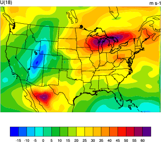
kl = 18
var = "U"
fg = first_guess->U
an = analysis->U
plot_data = an - fg
; plot_data = an
Then run the ncl script
ncl WRF-Var_plot.ncl
display WRF-VAR_U_level_18.pdf
You should see a plot similar to the one on the right.
|
 |
/kumquat/wrfhelp/DATA/WRFDA/TOOLS/graphics/ncl/plot_gts_omb_oma_simple.ncl can be used to plot the contents of gts_omb_oma_01.
cp /kumquat/wrfhelp/DATA/WRFDA/TOOLS/graphics/ncl/plot_gts_omb_oma_simple.ncl .
Edit plot_gts_omb_oma_simple.ncl to provide the date, filenames and options of your case.
......
plotdir = "ncl_plot/" ;where plot files will be created
expt = "my_plots" ; for output naming purposes, spaces are not allowed
datdir = "/kumquat/users/$USER/DA/3dvar/" ; the path of the working directory
......
fgname = "fg" ; for retrieving mapping info
......
Run the NCL script
ncl plot_gts_omb_oma_simple.ncl
This script may take a few minutes to complete; it will generate many plots depending on your settings. View the plots using display. An example of one of these plots, showing the OMA and OMB of sounding observations around 500 hPa, can be seen at right. Use spacebar and backspace to scroll through the different plots, showing OMB, OMA, and bias statistics for the observations at different pressure levels. There will be one output file per observation type; if you have time you can try plotting different observation types by editing the "proc_*" variables further down in the script.
|
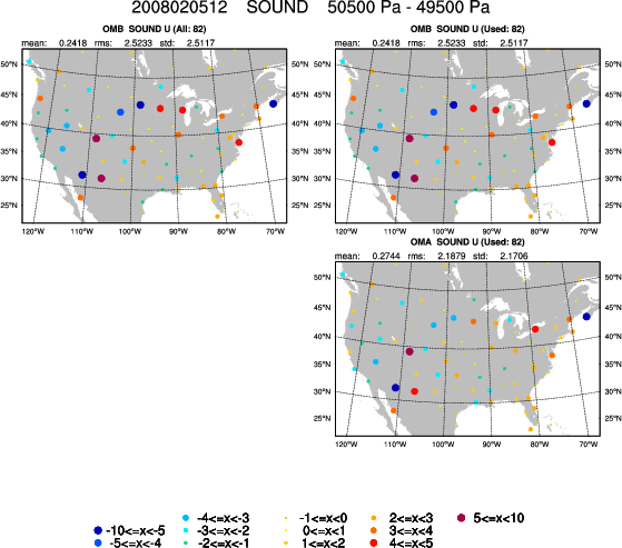 |
display ncl_plot/my_plots_sound_2008020512.pdf
There will be one output file per observation type; if you have time you can try plotting different observation types. You can also edit the "plevs" variable to change the way observations are arranged by pressure level.
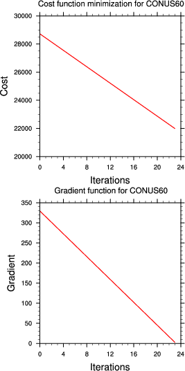
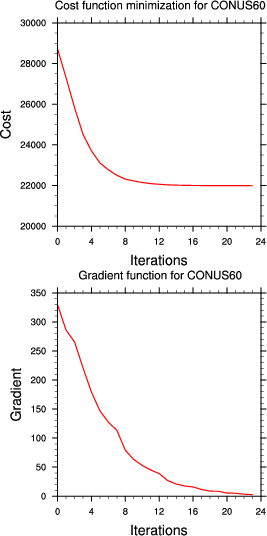
/kumquat/wrfhelp/DATA/WRFDA/TOOLS/graphics/ncl/plot_cost_grad_fn.ncl can be used to plot cost function evolution.
cp /kumquat/wrfhelp/DATA/WRFDA/TOOLS/graphics/ncl/plot_cost_grad_fn.ncl .
Edit plot_cost_grad_fn.ncl to provide the current working directory. You can also edit "domain_name" to change the plot captions.
......
dir = "/kumquat/users/$USER/DA/3dvar/"
domain_name = "my test case"
......
Run the NCL script
ncl plot_cost_grad_fn.ncl
You will notice that by default, WRFDA only prints information about the first and last iterations to cost_fn and grad_fn, so the plots will just be straight lines. If you wish to see more detailed plots, run the test case again, but with the option "calculate_cg_cost_fn = .true." under the &wrfvar11 namelist section.
Other WRF graphic tools can be used as well.
The full list of namelist options, including those not specified by the user (and so were assigned default values), can be found in the namelist.output.da file. Most of these options will not be useful for most purposes (e.g. the large list of "AUXINPUT" variables), so a more condensed list of WRFDA-related namelist options can be found at the end of the Users' Guide.
After creating an analysis, we have changed the initial conditions for the model. Therefore, if we want to use the analysis to create a forecast, the tendencies in the "wrfbdy" file should be adjusted based on these new initial conditions. This is done with da_update_bc.exe
Important: Make a copy of wrfbdy_d01 from this folder, do not simply link it. The wrf_bdy_file will be overwritten by da_update_bc.exe.
cp /kumquat/wrfhelp/DATA/WRFDA/CONUS60/rc/2008020512/wrfbdy_d01 ./wrfbdy_d01
Also, copy the sample da_update_bc namelist (parame.in) and make sure all the variables are set correctly for this experiment:
cp /kumquat/users/${USER}/DA/WRFDA/var/test/update_bc/parame.in .
vi parame.in
&control_param
da_file = './wrfvar_output'
wrf_bdy_file = './wrfbdy_d01'
wrf_input = '/kumquat/wrfhelp/DATA/WRFDA/CONUS60/rc/2008020512/wrfinput_d01'
domain_id = 1
cycling = .false.
debug = .true.
low_bdy_only = .false.
update_lsm = .false.
var4d_lbc = .false.
/
Run da_update_bc.exe
/kumquat/users/${USER}/DA/WRFDA/var/build/da_update_bc.exe
Finally, check the output. Use diffwrf (available in compiled WRFV3 code at WRFV3/external/io_netcdf/diffwrf), ncdiff, ncview, or other WRF NCL graphic tools to check what fields have been updated.
The wrfvar_output and wrfbdy_d01 are the data-assimilated initial condition and tendency-updated boundary condition for your subsequent WRF model run. You will learn more about this in the cycling exercises later this week.
You are now finished with the basic exercise for WRFDA-3DVAR with real data. You can now continue to the next practice case.
You can come back here later for additional practice running WRFDA-3DVAR with real data below: