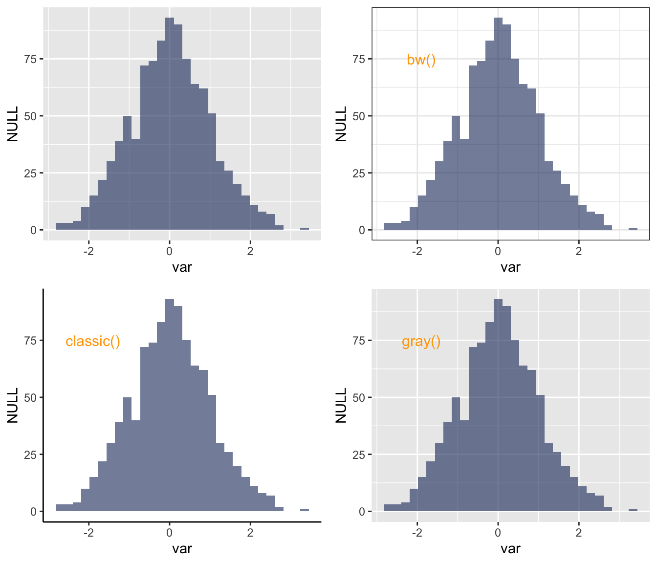
Themes provided by ggplot2
Two main types of grid exist with ggplot2: major and minor. They are controled thanks to the panel.grid.major and panel.grid.minor options.
Once more, you can add the options .y or .x at the end of the function name to control one orientation only.
Features are wrapped in an element_line() function. Specifying element_blanck() will simply removing the grid.
# library
library(ggplot2)
library(gridExtra)
# create data
set.seed(123)
var=rnorm(1000)
# Without theme
plot1 <- qplot(var , fill=I(rgb(0.1,0.2,0.4,0.6)) )
# With themes
plot2 = plot1+theme_bw()+annotate("text", x = -1.9, y = 75, label = "bw()" , col="orange" , size=4)
plot3 = plot1+theme_classic()+annotate("text", x = -1.9, y = 75, label = "classic()" , col="orange" , size=4)
plot4 = plot1+theme_gray()+annotate("text", x = -1.9, y = 75, label = "gray()" , col="orange" , size=4)
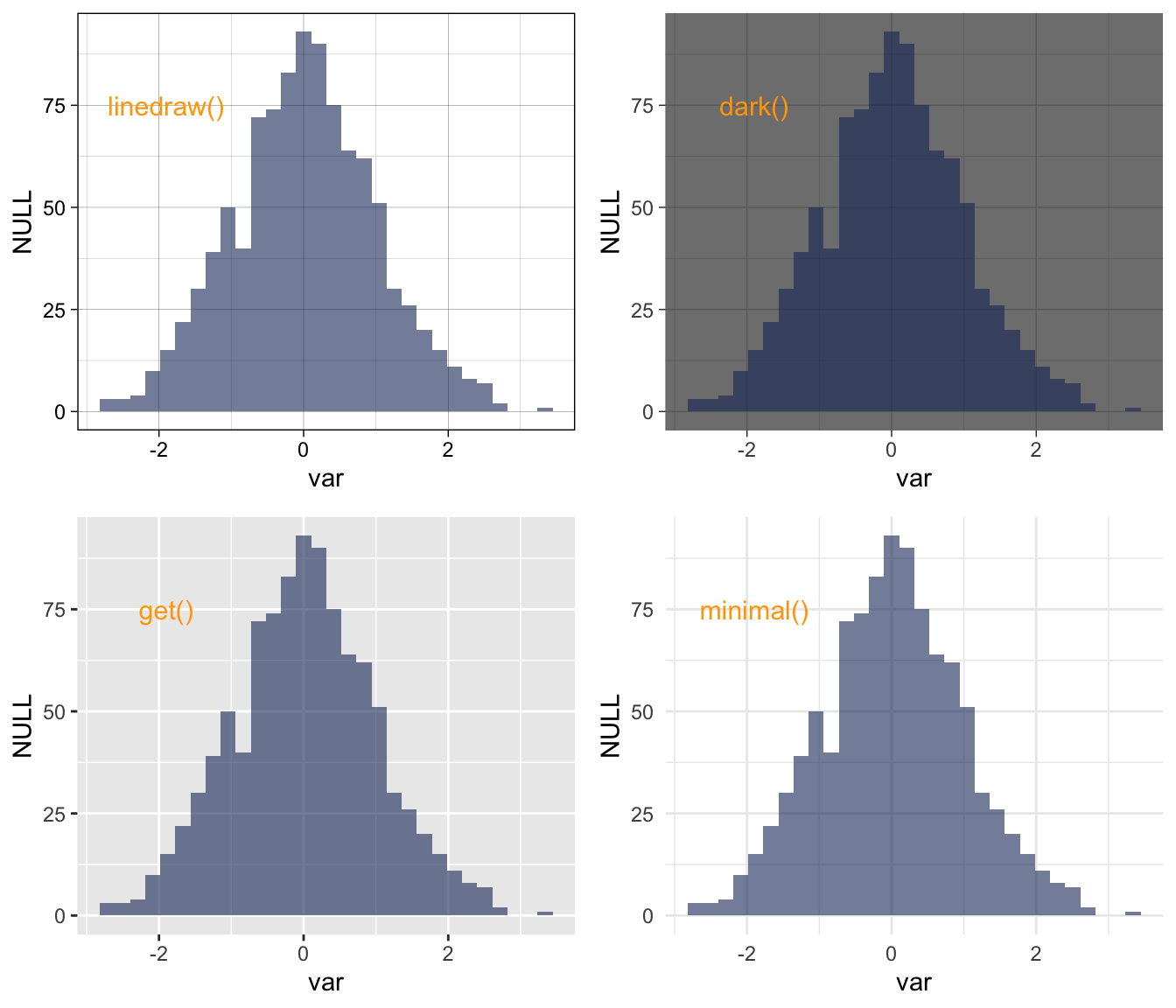
plot5 = plot1+theme_linedraw()+annotate("text", x = -1.9, y = 75, label = "linedraw()" , col="orange" , size=4)
plot6 = plot1+theme_dark()+annotate("text", x = -1.9, y = 75, label = "dark()" , col="orange" , size=4)
plot7 = plot1+theme_get()+annotate("text", x = -1.9, y = 75, label = "get()" , col="orange" , size=4)
plot8 = plot1+theme_minimal()+annotate("text", x = -1.9, y = 75, label = "minimal()" , col="orange" , size=4)
# Arrange and display the plots into a 2x1 grid
grid.arrange(plot1,plot2,plot3,plot4, ncol=2)Code used for the ggplot2 page.
Here is the code used for the examples displayed on the ggplot2 page. It shows how to used most of the common packages related to ggplot2 themes.
# library
library(ggplot2)

# My margini
mytheme <- theme(
      plot.margin=unit(rep(1.3,4),"cm")
      )

# Plot
p <- ggplot(iris, aes(x=Sepal.Length, y=Sepal.Width, color=Species, shape=Species)) +
    geom_point(size=6, alpha=0.6, show.legend = FALSE)

setwd("~/Desktop/R-graph-gallery/img/graph")
png("192-ggplot-theme_default.png") ;  p + mytheme ; dev.off()
png("192-ggplot-theme_bw.png") ;  p + theme_bw() + mytheme ; dev.off()
png("192-ggplot-theme_minimal.png") ;  p + theme_minimal() + mytheme ; dev.off()
png("192-ggplot-theme_classic.png") ;  p + theme_classic() + mytheme ; dev.off()
png("192-ggplot-theme_gray.png") ;  p + theme_gray() + mytheme ; dev.off()

#library(ggthemes)
png("192-ggplot-theme_excel.png") ;  p + theme_excel() + mytheme ; dev.off()
png("192-ggplot-theme_economist.png") ;  p + theme_economist() + mytheme ; dev.off()
png("192-ggplot-theme_fivethirtyeight.png") ;  p + theme_fivethirtyeight() + mytheme ; dev.off()
png("192-ggplot-theme_tufte.png") ;  p + theme_tufte() + mytheme ; dev.off()
png("192-ggplot-theme_gdocs.png") ;  p + theme_gdocs() + mytheme ; dev.off()
png("192-ggplot-theme_wsj.png") ;  p + theme_wsj() + mytheme ; dev.off()
png("192-ggplot-theme_calc.png") ;  p + theme_calc() + scale_colour_calc() + mytheme ; dev.off()
png("192-ggplot-theme_hc.png") ;  p + theme_hc() + scale_colour_hc() + mytheme ; dev.off()

# library(hrbrthemes)
png("192-ggplot-theme_ipsum.png") ;  p + theme_ipsum() + scale_color_ipsum() + mytheme ; dev.off()

# library(egg)
png("192-ggplot-theme_article.png") ;  p + theme_article() + mytheme ; dev.off()

# library(ggpubr)
png("192-ggplot-theme_pubclean.png") ;  p + theme_pubclean() + mytheme ; dev.off()
# library(bigstatsr)
png("192-ggplot-theme_bigstatsr.png") ;  p + theme_bigstatsr() + mytheme ; dev.off()


png("192-ggplot-theme_excel.png") ;  p + theme_excel() + mytheme ; dev.off()
png("192-ggplot-theme_excel.png") ;  p + theme_excel() + mytheme ; dev.off()
png("192-ggplot-theme_excel.png") ;  p + theme_excel() + mytheme ; dev.off()
png("192-ggplot-theme_excel.png") ;  p + theme_excel() + mytheme ; dev.off()
png("192-ggplot-theme_excel.png") ;  p + theme_excel() + mytheme ; dev.off()
png("192-ggplot-theme_excel.png") ;  p + theme_excel() + mytheme ; dev.off()
png("192-ggplot-theme_excel.png") ;  p + theme_excel() + mytheme ; dev.off()

theme_bigstatsr()