Compute the correlation matrix
Consider a dataset composed by entities (usually in rows) and features (usually in columns).
It is possible to compute a correlation matrix from it. It is a square matrix showing the relationship between each pair of entity. It can be computed using correlation (cor()) or euclidean distance (dist()).
Let’s apply it to the mtcars dataset that is natively provided by R.
# library
library(igraph)

# data
# head(mtcars)

# Make a correlation matrix:
mat <- cor(t(mtcars[,c(1,3:6)]))
Basic network diagram
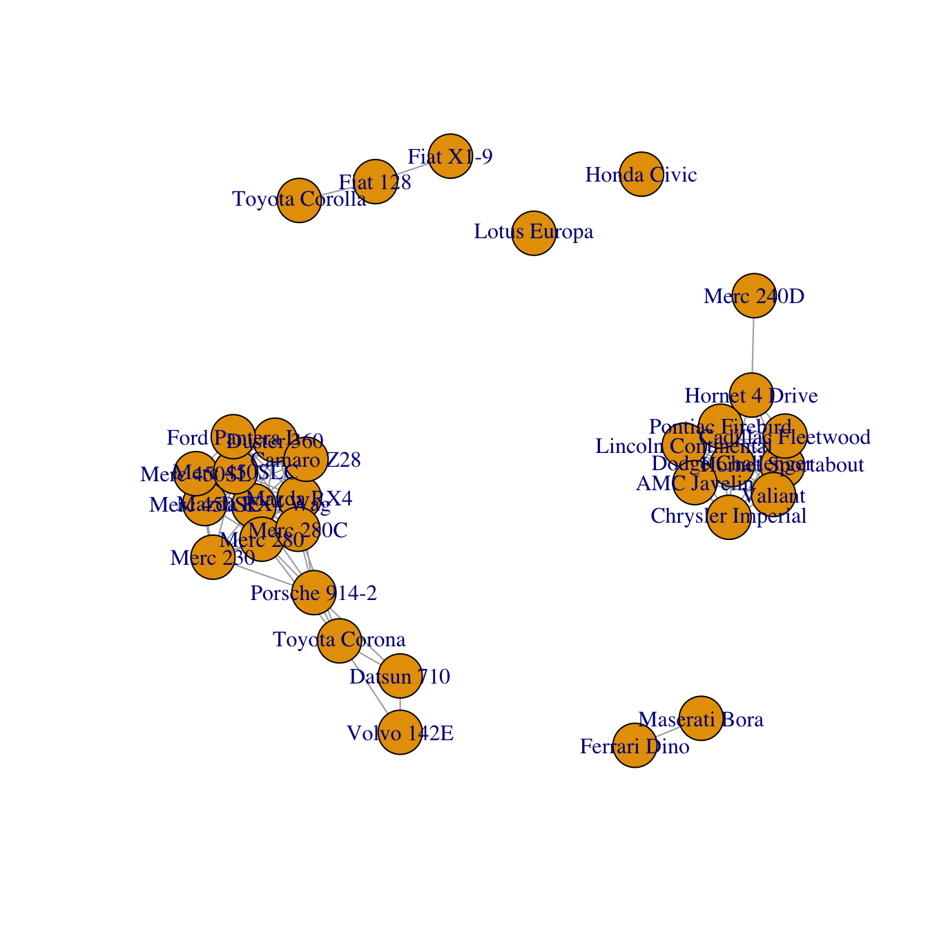
A correlation matrix can be visualized as a network diagram. Each entity of the dataset will be a node. And 2 nodes will be connected if their correlation or distance reach a threshold (0.995 here).
To make a graph object from the correlation matrix, use the graph_from_adjacency_matrix() function of the igraph package. If you’re not familiar with igraph, the network section is full of examples to get you started.
# Keep only high correlations
mat[mat<0.995] <- 0

# Make an Igraph object from this matrix:
network <- graph_from_adjacency_matrix( mat, weighted=T, mode="undirected", diag=F)

# Basic chart
plot(network)
Customization
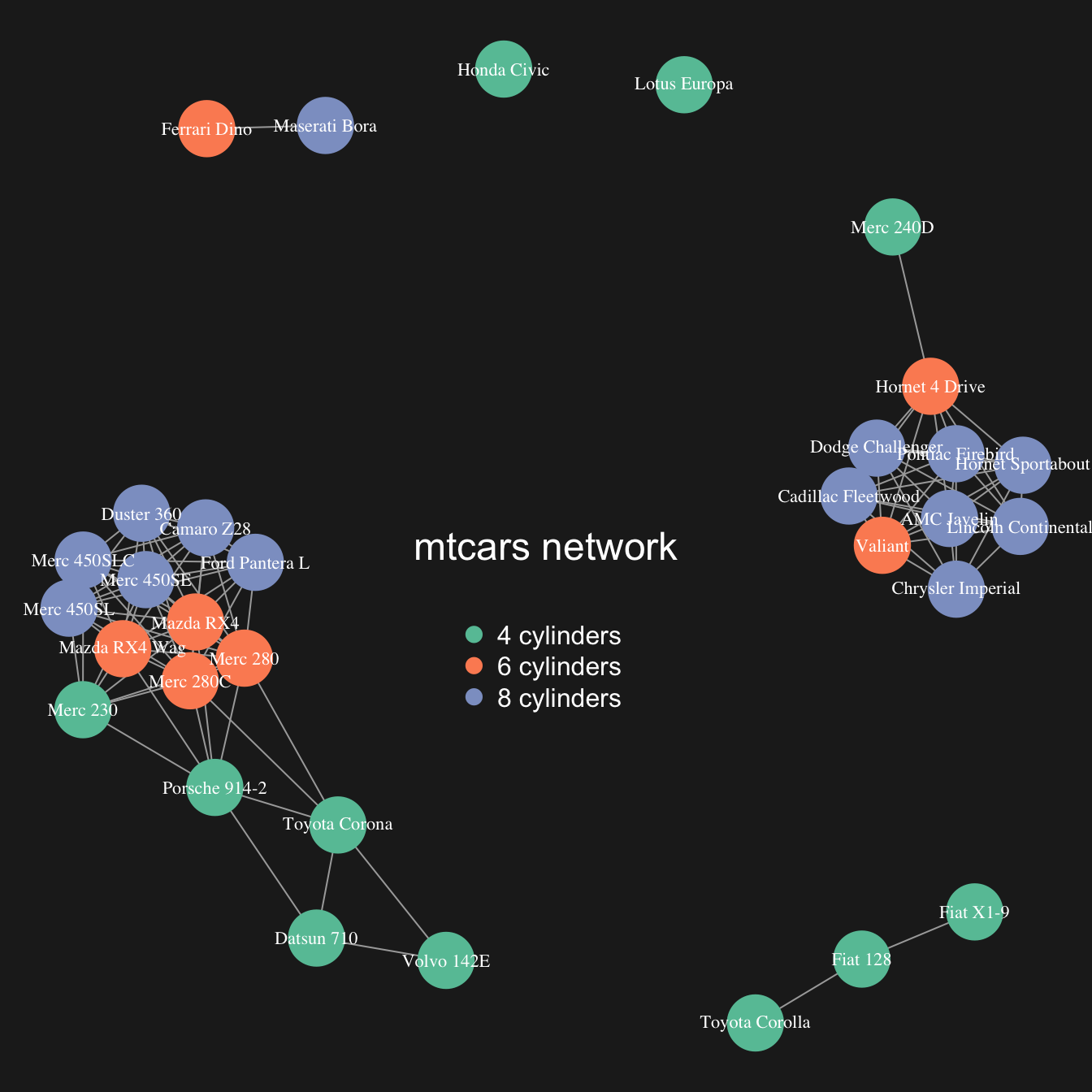
The hardest part of the job has been done. The chart just requires a bit of polishing for a better output:
- customize node, link, label and background features as you like
- map the node feature to a variable (
cylhere). It gives an additional layer of information, allowing to compare the network structure with a potential expected organization.
# color palette
library(RColorBrewer)
coul <- brewer.pal(nlevels(as.factor(mtcars$cyl)), "Set2")

# Map the color to cylinders
my_color <- coul[as.numeric(as.factor(mtcars$cyl))]

# plot
par(bg="grey13", mar=c(0,0,0,0))
set.seed(4)
plot(network,
    vertex.size=12,
    vertex.color=my_color,
    vertex.label.cex=0.7,
    vertex.label.color="white",
    vertex.frame.color="transparent"
    )

# title and legend
text(0,0,"mtcars network",col="white", cex=1.5)
legend(x=-0.2, y=-0.12,
       legend=paste( levels(as.factor(mtcars$cyl)), " cylinders", sep=""),
       col = coul ,
       bty = "n", pch=20 , pt.cex = 2, cex = 1,
       text.col="white" , horiz = F)
Customize link features
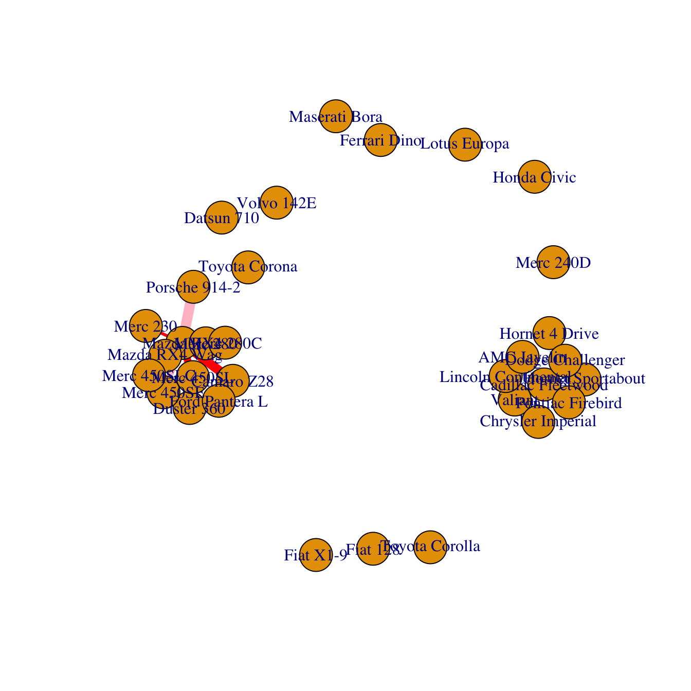
Last but not least, control edges with arguments starting with edge..
plot(network,
edge.color=rep(c("red","pink"),5), # Edge color
edge.width=seq(1,10), # Edge width, defaults to 1
edge.arrow.size=1, # Arrow size, defaults to 1
edge.arrow.width=1, # Arrow width, defaults to 1
edge.lty=c("solid") # Line type, could be 0 or “blank”, 1 or “solid”, 2 or “dashed”, 3 or “dotted”, 4 or “dotdash”, 5 or “longdash”, 6 or “twodash”
#edge.curved=c(rep(0,5), rep(1,5)) # Edge curvature, range 0-1 (FALSE sets it to 0, TRUE to 0.5)
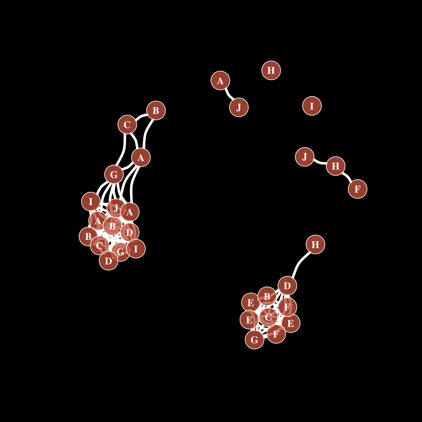
)All customization
Of course, you can use all the options described above all together on the same chart, for a high level of customization.
par(bg="black")

plot(network,

    # === vertex
    vertex.color = rgb(0.8,0.4,0.3,0.8),          # Node color
    vertex.frame.color = "white",                 # Node border color
    vertex.shape="circle",                        # One of “none”, “circle”, “square”, “csquare”, “rectangle” “crectangle”, “vrectangle”, “pie”, “raster”, or “sphere”
    vertex.size=14,                               # Size of the node (default is 15)
    vertex.size2=NA,                              # The second size of the node (e.g. for a rectangle)

    # === vertex label
    vertex.label=LETTERS[1:10],                   # Character vector used to label the nodes
    vertex.label.color="white",
    vertex.label.family="Times",                  # Font family of the label (e.g.“Times”, “Helvetica”)
    vertex.label.font=2,                          # Font: 1 plain, 2 bold, 3, italic, 4 bold italic, 5 symbol
    vertex.label.cex=1,                           # Font size (multiplication factor, device-dependent)
    vertex.label.dist=0,                          # Distance between the label and the vertex
    vertex.label.degree=0 ,                       # The position of the label in relation to the vertex (use pi)

    # === Edge
    edge.color="white",                           # Edge color
    edge.width=4,                                 # Edge width, defaults to 1
    edge.arrow.size=1,                            # Arrow size, defaults to 1
    edge.arrow.width=1,                           # Arrow width, defaults to 1
    edge.lty="solid",                             # Line type, could be 0 or “blank”, 1 or “solid”, 2 or “dashed”, 3 or “dotted”, 4 or “dotdash”, 5 or “longdash”, 6 or “twodash”
    edge.curved=0.3    ,                          # Edge curvature, range 0-1 (FALSE sets it to 0, TRUE to 0.5)
    )