---
title: "STAT 302 Statistical Computing"
subtitle: "Lecture 1: Introduction and R Basics"
author: "Yikun Zhang (_Winter 2024_)"
date: ""
output:
xaringan::moon_reader:
css: ["uw.css", "fonts.css"]
lib_dir: libs
nature:
highlightStyle: tomorrow-night-bright
highlightLines: true
countIncrementalSlides: false
titleSlideClass: ["center","top"]
---
```{r setup, include=FALSE, purl=FALSE}
options(htmltools.dir.version = FALSE)
knitr::opts_chunk$set(comment = "##")
library(kableExtra)
```
# Outline
1. Course Overview
2. Introduction to R, RStudio, and R Markdown
3. Elementary Operations in R
4. Data Types in R
Appendices:
A. Probability
B. Random Variables
* Acknowledgement: Parts of the slides are modified from the course materials by Prof. Ryan Tibshirani, Prof. Yen-Chi Chen, Prof. Deborah Nolan, Bryan Martin, and Andrea Boskovic.
---
class: inverse
# Part 1: Course Overview and Logistics
---
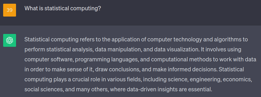
# What Is Statistical Computing?
--
Answer: A computing program that does Statistics!
Well! Let's see some "official answers"...
--
From ChatGPT:
---
# What Is Statistical Computing?
--
Statistical computing is a course with intensive programming tasks that are related to Statistics.
--
In other words, there will be a lot of coding in this course!!
---
# Why Do We Learn Statistical Computing?
--
- We want to utilize (big) data to address scientific questions.

Cited from
https://bleuwire.com/5-biggest-big-data-challenges/.
---
# Why Do We Learn Statistical Computing?
**An Example From My Research**: Cosmic Web Detection with Observed Galaxies in the Sloan Digital Sky Survey.
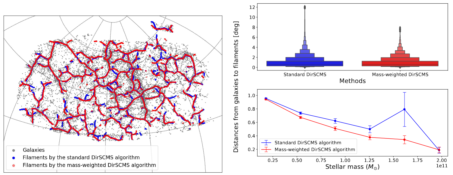
See my paper at
MNRAS and our cosmic web catalog (i.e., a well-documented dataset).
One scientific question that we address here is "*how is the stellar mass of a galaxy correlated with its distance to nearby cosmic web structures?*"
---
# Why Do We Learn Statistical Computing?
- We need to conduct simulation studies to validate our statistical theory and methodology.
--
- For example, we can verify the asymptotic normality of our proposed statistical estimator with finite samples.
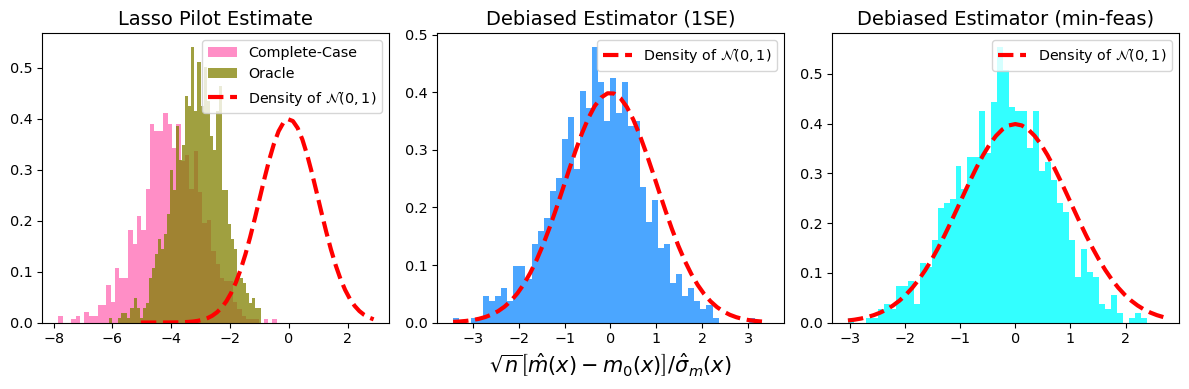
See my recent paper
https://arxiv.org/abs/2309.06429.
---
# Why Do We Learn Statistical Computing?
- Mastering statistical computing skills can give us better jobs.
--

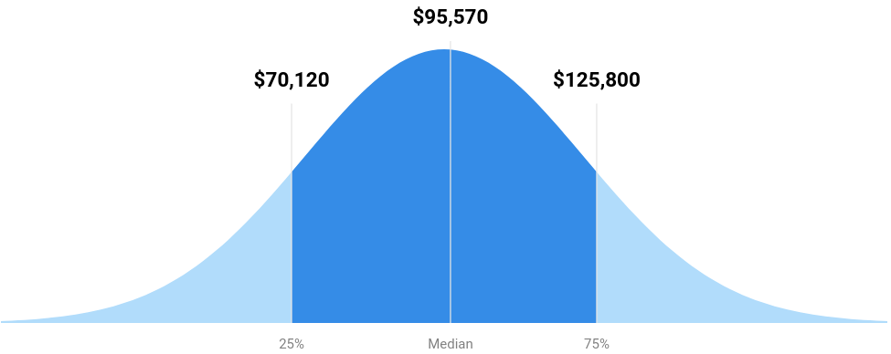
Sources from US News in 2021.
---
# Syllabus

Let's spend some time going over the [Course Syllabus](https://zhangyk8.github.io/teaching/file_stat302/Syllabus_Win2024.pdf).
---
# Canvas Discussion
* It is worth up to 2% extra credit on the final grade.
* Only substantive and helpful questions will be counted.
.pull-left[
### Bad questions:
* How do you do Problem 2?
* Here's my code and it's broken. How can I fix it?
]
--
.pull-right[
### Good questions:
* Here's a snippet of code that I used for Problem 2:
`formatted code snippet`
It returned the following error:
`formatted error message`
Does anyone know why? I already tried...
* I don't understand the concept from Slide 18 today. Could anyone elaborate on why...?
]
---
# Canvas Discussion
* It is worth up to 2% extra credit on the final grade.
* Only substantive and helpful answers will be counted.
.pull-left[
### Bad or null answers:
* Here's my solution:
`formatted code snippet`
* The grader is wrong. You should ask the grader to add your points back...
(*However, you are encouraged to point out my mistakes and typos during lectures or on the discussion board.*)
]
--
.pull-right[
### Good answers:
* This error message occurs because your variable is a string instead of a numeric.
Have you tried checking...?
* I think that Slide 18 in Lecture 2 will address your questions.
]
---
# Why R?
R is a programming language developed by statisticians for statistical computing.
### Pros:
* R is open-source and has a community of developers and users.
* It is convenient for statistical analysis and data visualization...

--
### Cons:
* R is slow unless we use parallel computing packages or [Rcpp](https://www.rcpp.org/).
* It is not very popular outside of the statistical community.
---
# Why R?
.pull-left[
Windows Interface
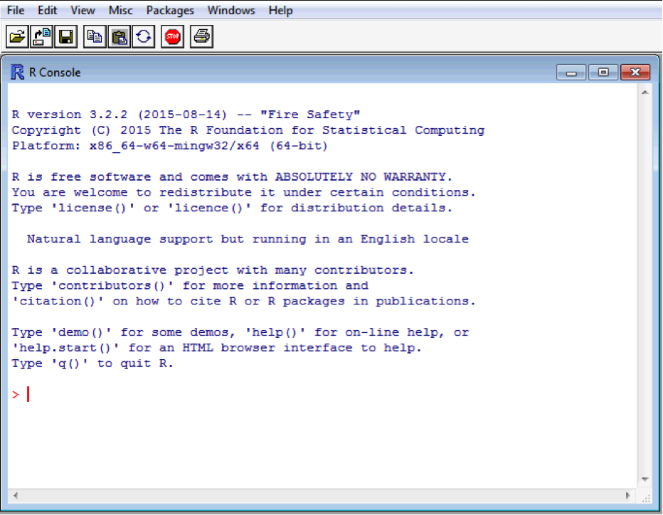
]
.pull-right[
Linux/Unix Terminal

]
--
It is not convenient to write programs with thousands of R code lines directly in the R interface!
---
# Why RStudio?
Luckily, we have [RStudio](https://posit.co/download/rstudio-desktop/), an integrated development environment (IDE) designed for writing and running R programming.
--
* We recommend to first install R. Then, Rstudio will automatically locate the R directory in our computer.
* It helps us organizes R scripts, files, plots, code console, etc.
* It provides helpful interactive graphical interface.
--
* And more essentially, it has R Markdown integration.
For the rest of the course, we will use Rstudio to write our code and finish the lab assignments.
---
# RStudio Interface
By default...
* *Top left*: Editor panel. Browse and edit scripts or data with tabs.
* *Top right*: List of objects in the Environment (recall `ls()`), code history, etc.
* *Bottom left*: Console for running R code line-by-line (`>` prompt)
* *Bottom right*: Files, plots, packages, help files, etc.
If the Edit window is not open, then choose File -> New File -> Choose R Script.
---
# Editor
* Our important code should be written here (**not** the console).
* Primarily used for writing and editing .R or .Rmd scripts.
* Try opening a file now using *File > New File > R Script*, write two lines of simple code, such as `1 + 3` or `a = 6`.
* Click `Run` in the bar above the script. What happens?
* Click on one of the lines of code. Press `Ctrl`/`⌘` + `Enter`. What happens?
--
.center[**Important:** Every part of our R workflow belongs in this window!]
---
# Console and Environment/History
#### Console
* It gives us an easy way to run and test individual lines of code.
* Nothing that we run here will be saved after we close Rstudio (unless you save the R history)!
--
#### Environment/History
* The variables that we defined can be seen in the _Environment_ tab.
* Click on the _History_ tab to see what it contains. Try searching!
* Select a line from the _History_ tab and click `To Source`. What happens?
- It is useful for adding lines that we tested in our Console to our R scripts.
---
# Files, Plots, Packages, Help
* _Files_ tab is used to browse the files on our computer.
* Open files/data, move files that we are working with, etc.
* **Use caution!** Changing files here is the same as changing them on our computer. If we delete something, it's gone!
* _Plots_ tab is used to display plots that we create in R.
* _Help_ tab is used to browse the documentations of functions. We can explore these by preceding a function name with `?`.
Try `?sqrt` to see its user documentation. (If we are unsure about any function, ask R in this way!)
* _Packages_ tab shows all the packages that we currently have installed. (We will discuss more about it later.)
---
# Why R Markdown?
[R Markdown](https://rmarkdown.rstudio.com/) is a markup language for combining R code with text.
* It facilitates the creations of those neat HTML files, PDF documents, slides (like the one I am using), webpages, books, etc.
--
* And more importantly, it is required for our lab assignments and final project!
---
# Create an R Markdown File
Let's try creating an R Markdown file:
1. Choose *File > New File > R Markdown...*.
2. Make sure *PDF Output* is selected and click OK.
3. Save the file in your new folder, call it `stat302_test1.Rmd`.
4. Click the *Knit* button
* After it is done, browse to the file location using the `Files` tab. What have been added?
Note: The PDF output requires an installation of $\LaTeX$; see the instructions [here](https://bookdown.org/yihui/rmarkdown/installation.html).
---
# R Markdown Syntax
.pull-left[
## Output
**bold/strong emphasis**
*italic/normal emphasis*
.forcehead[Header]
## Subheader
### Subsubheader
]
.pull-right[
## Syntax
**bold/strong emphasis**

*italic/normal emphasis*

# Header

## Subheader

### Subsubheader
]
---
# R Markdown Syntax
.pull-left[
## Output
1. Ordered list Item 1
1. Item 2
1. Even with sub-item 1
2. Sub-item 2
* Unordered lists Item 1
* Item 2
+ Sub-item
[URL link](http://www.uw.edu)

]
.pull-right[
## Syntax
1. Ordered list Item 1
1. Item 2
1. Even with sub-item 1
2. Sub-item 2
* Unordered lists Item 1
* Item 2
+ Sub-item
[URL link](http://www.uw.edu)

]
---
# R Markdown Syntax
.pull-left[
## Output
You can put some math $y= \left( \frac{5}{3} \right)^2$ right up in there.
$$\frac{1}{n} \sum_{i=1}^{n} x_i = \bar{x}_n$$
Or a sentence with `code-looking font`.
Or a block of code:
```
y <- 1:5
z <- y^2
```
]
.pull-right[
## Syntax
You can put some math $y= \left(\frac{5}{3}
\right)^2$ right up in there

$$\frac{1}{n} \sum_{i=1}^{n}
x_i = \bar{x}_n$$

Or a sentence with `code-looking font`.

Or a block of code:

    ```
    y <- 1:5
    z <- y^2
    ```
]
---
# R Code Within R Markdown
As in Lab 1, we can run and execute R code within R Markdown.
To do so, we need to encase our code as follows.
`r ''````{r, eval = TRUE, echo = TRUE}
# Your code goes here!
```
We can click the green triangle in the corner to evaluate that code chunk to preview the results without compiling the entire document.
---
# Useful Code Chunk Parameters
Parameters go into the opening brackets `{r}` and are separated by commas. Here are some useful options:
* `echo=FALSE`: Hide R code but keep results.
* `eval=FALSE`: Do not execute the R code.
* `include=FALSE`: Hide all outputs for this chunk (It is useful to load packages at the beginning of your document).
* `cache=TRUE`: Store the results of the chunk, and only re-run if the chunk is changed. (It is useful for files that take a while to compile).
* `fig.height=5, fig.width=5`: Modify the dimensions of any plots that are generated in the chunk (units are in inches).
Note: See the [R Markdown Reference Guide](https://www.rstudio.com/wp-content/uploads/2015/03/rmarkdown-reference.pdf) for a complete list of knitr chunk options.
---
class: inverse
# Part 2: R Basics
---
# R as a Calculator
* **Binary (Arithmetic) Operators** take two arguments. For instance, +, -, *, /, %% (for mod), %/%(integer division), and ^ (exponentiation).
```{r}
# Addition
6 + 1
```
```{r}
# Subtraction
9 - 16.6
```
```{r}
# Multiplication
6 * 3
```
---
# R as a Calculator
* **Binary (Arithmetic) Operators** take two arguments. For instance, +, -, *, /, %% (for mod), %/% (integer division), and ^ (exponentiation).
```{r}
# Division
10 / 3
```
```{r}
# Mod
10 %% 3
```
```{r}
# Integer division
10 %/% 3
```
---
# R as a Calculator
* **Binary (Arithmetic) Operators** take two arguments. For instance, +, -, *, /, %% (for mod), %/% (integer division), and ^ (exponentiation).
```{r}
# Exponentiation
3^4
```
```{r}
# Exponentiation (same as the syntax in Python)
3**4
```
* **Unitary (Arithmetic) Operators** take only one argument. For example, - is for arithmetic negation.
---
# R as a Calculator
* We can also use some built-in functions in R to calculate more advanced math functions.
```{r}
# Exponentiation with natural basis "e"
exp(3)
```
```{r}
# Trigonometric functions
sin(pi)
cos(2*pi)
```
---
# R as a Calculator
```{r}
# Square root
sqrt(5)
```
```{r}
# Logarithm with natural base
log(10)
```
```{r}
# Logarithm with base 10
log(10, base=10)
# Ask R (in the console) if we are unsure of
# any function and its arguments
?log
```
---
# Comparison Operators
```{r}
# Strictly greater than
6 > 3
# Greater than or equal to
6 >= 6
```
```{r}
# Equal to
5 == 3
5 == 2 + 3
```
---
# Comparison Operators
```{r}
# Not equal to
6 != 3
```
```{r}
# Strictly less than
6 < 6
# Less than or equal to
6 <= 6
```
---
# Logical Operators
* **Logical Operators** take one or more "comparison statements" and return TRUE or FALSE.
```{r}
# AND
(6 < 5) & (1 < 3)
```
```{r}
# AND
(6 < 9) & (1 <= 3)
```
---
# Logical Operators
* **Logical Operators** take one or more "comparison statements" and return TRUE or FALSE.
```{r}
# OR
(6 < 5) | (1 < 3)
```
```{r}
# OR
(6 < 5) | (1 <= -3)
```
```{r eval=FALSE}
# Combine AND with OR operators
(6 < 5) & (7 > 2) | (1 <= 3)
```
--
```{r echo=FALSE}
# Combine AND with OR operators
(6 < 5) & (7 > 2) | (1 <= 3)
```
---
# Logical Operators
* **Logical Operators** take one or more "comparison statements" and return TRUE or FALSE.
```{r}
# Logical negation
!(6 < 5)
```
```{r}
# Logical negation
!(6 < 9)
```
---
class: inverse
# Part 3: Data Types in R
---
# Functional Programming
Functional programming in R comprises two basic types of things/objects: **data** and **functions**.
--
* **Data** are things like 8, "James", *NA*, and
$$\begin{bmatrix}
1 & 3 & 6\\
4 & 7 & -1\\
\end{bmatrix}.$$
--
* **Functions** are some programs that turns input objects, or *arguments*, into an output object or a return value (possibly with side effects), according to a definite rule.
--
* Good programming is writing functions to correctly and efficiently transform inputs into outputs. (We will discuss functions later...)
- The principle of good programming is to take a big transformation and break it down into smaller ones so that we can efficiently implement these smaller tasks (using built-in functions).
---
# Data Types
At the base level, all data can represented in binary format, by **bits** (i.e., TRUE/FALSE, YES/NO, 1/0). However, basic data types in R are:
- **Booleans** are direct binary values: `TRUE` or `FALSE` in R.
- **Integers** are whole numbers (positive, negative or zero), represented by a fixed-length block of bits.
- **Floating point numbers** are (some approximations) to rational numbers, i.e., $p/q$ where $p,q$ are both integers.
- **Complex numbers** are numbers like 1+2i.
- **Characters** are fixed-length blocks of bits, with special coding; **strings** are sequences of characters.
- **Missing or ill-defined values**: `NA`, `NaN`, etc.
---
# Data Types (Examples)
```{r}
?typeof()
typeof(TRUE)
# By default, R stores numeric values as 64 floating points.
typeof(6)
# We can coerce it into integer as follows.
typeof(as.integer(6))
typeof(as.integer(6.5))
```
---
# Data Types (Examples)
We can also use the built-in function `class()` to determine the data type of an object. [This webpage](https://stackoverflow.com/questions/6258004/types-and-classes-of-variables) describes the differences between `typeof()` and `class()`.
- In short, `typeof()` or `mode()` represents how an object is stored in memory (numeric, character, list, or function), while `class()` represents its abstract type.
```{r}
class(6)
typeof(6)
mode(6)
```
---
# Data Types (Examples)
```{r}
as.integer(6.6)
# It rounded a floating point number 6.5 to the largest integer that is less than 6.5. Check its difference with the `ceiling()` function.
floor(6.6)
typeof("7")
length("7112")
```
---
# Data Types (Examples)
```{r}
is.character("7")
is.na(6.6)
is.na(NA)
```
--
```{r}
is.na(NaN)
is.nan(NA)
```
---
# Variables in R
- With the preceding arithmetic operations, it is difficult for us to utilize the outputs.
--
- To better keep track of the intermediate results, we can assign the (outputs of) expressions to some **named variables**.
- Naming variables is the first step towards abstraction in functional programming.
--
```{r}
a = 1 + 2
course_code = "STAT 302"
dept = paste("Statistics", "Data Science")
# List all the variables that we have defined
ls()
```
Note: `<-` and `=` are both valid assignment operators.
---
# Variables in R
* A variable in R has its name and value.
* We can access a variable by its name.
```{r}
# Access variable `a`
a
# Check the data type of `course_code`
class(course_code)
```
--
```{r}
# Remove a variable (from R memory)
rm("a")
```
Note: We can also keep track of all the defined variables in the _Environment_ tab (**Top right** in Rstudio).
---
# Rules for Variable's Name
* A variable's name must follow some rules:
- It cannot start with a digit or underscore `_`.
- It may contain characters, digits, and some punctuation (period `.` and underscore `_` are allowed, while others are generally prohibited).
- It is case-sensitive.
--
```{r}
w2v = 1 + 4
W2v = "word to vector"
w2v == W2v
```
---
# Summary
- Statistical computing focuses on using the computer programs to solve scientific problems with solid statistical methods.
- R is an open-source programming language for statistical computing.
- RStudio and R markdown further enhance our R programming experience.
- R supports arithmetic, comparison, and logical operators.
- The basic data types in R enable us to represent Booleans, numbers, characters, etc.
Submit Lab 1 on Gradescope by the end of Monday (January 15)!!
---
class: inverse
# Appendix A. Probability
---
# Sample Space
A **sample space**, commonly denoted $\Omega$ or $S$, is the set of all possible outcomes from a random experiment. For example,
* Coin flip: $\Omega = \{H, T\}$;
* Two coin flips: $\Omega = \{HH, HT, TH, TT\}$;
* Rolling a 6-sided die: $\Omega = \{1, 2, 3, 4, 5, 6\}$;
* Hours spent sleeping in day: $\Omega = \{x: x\in \mathbb{R}, 0 \leq x \leq 24\}$;
* A simulation from a normal distribution: $\Omega = (-\infty, \infty)$.
The elements of $\Omega$ must be **mutually exclusive** and **collectively exhaustive**.
---
# Events
An **event**, which we will call $A$, can be any subset of your sample space. For example,
* Heads in a coin flip: $A = \{H\}$;
* At least one heads in two coin flips: $A = \{HT, HT, TH\}$;
* Rolling an even number on a 6-sided die: $A = \{2, 4, 6\}$;
* Sleeping at least 8 hours in a day: $A = \{x: x \in \mathbb{R}, 8 \leq x \leq 24\}$;
* Simulating a number between 1 and 2, inclusive, from a normal distribution: $A = [1, 2]$.
---
# Probability
Informally, probability $P$ is often defined as the chance of something happening.
More formally, it is a function that goes from an event $A$ to the real line.
* $P(\text{heads in a fair coin flip}) = \dfrac{1}{2}$.
* $P(\text{at least one heads in two fair coin flips}) = \dfrac{3}{4}$.
* $P(\text{rolling an even number on a fair dice}) = \dfrac{1}{2}$.
---
# Axioms of Probability
Probability allows follows three basic principles, known as the **axioms of probability**.
1. The probability of any event $A$ must be between 0 and 1, inclusive.
* $0 \leq P(A)\leq 1$.
2. The probability of the sample space is equal to 1.
* $P(\Omega) = 1$.
3. If events $A$ and $B$ are **mutually exclusive**/**disjoint**, then the probability of *either* $A$ *or* $B$ is the same as the sum of the probability of $A$ and the probability of $B$.
* $A \cap B = \emptyset \ \ \Rightarrow \ \ P(A\cup B) = P(A) + P(B)$
---
layout: true
# Probability Notation
---
## Intersection: $\cap$
$P(A \cap B)$: *joint* probability of $A$ *and* $B$.
.center[ ]
---
## Intersection: $\cap$
$P(A \cap B)$: *joint* probability of $A$ *and* $B$.
.center[
]
---
## Intersection: $\cap$
$P(A \cap B)$: *joint* probability of $A$ *and* $B$.
.center[ ]
---
## Union: $\cup$
$P(A \cup B)$ probability of $A$ *or* $B$.
.center[]
---
## Union: $\cup$
$P(A \cup B)$ probability of $A$ *or* $B$.
.center[
]
---
## Union: $\cup$
$P(A \cup B)$ probability of $A$ *or* $B$.
.center[]
---
## Union: $\cup$
$P(A \cup B)$ probability of $A$ *or* $B$.
.center[ ]
---
## Complement: $A^c$
$P(A^c)$ probability of *not* $A$.
.center[]
---
## Complement: $A^c$
$P(A^c)$ probability of *not* $A$.
.center[
]
---
## Complement: $A^c$
$P(A^c)$ probability of *not* $A$.
.center[]
---
## Complement: $A^c$
$P(A^c)$ probability of *not* $A$.
.center[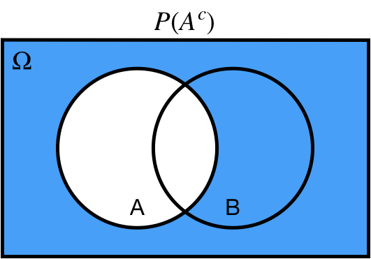 ]
---
## Difference: $A\setminus B$
$P(A\setminus B)$ probability of $A$ *and not* $B$.
.center[]
---
## Difference: $A\setminus B$
$P(A\setminus B)$ probability of $A$ *and not* $B$.
.center[
]
---
## Difference: $A\setminus B$
$P(A\setminus B)$ probability of $A$ *and not* $B$.
.center[]
---
## Difference: $A\setminus B$
$P(A\setminus B)$ probability of $A$ *and not* $B$.
.center[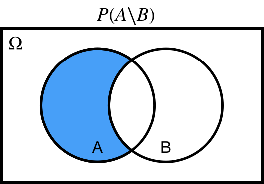 ]
---
## Conditional: $A | B$
$P(A | B)$ probability of $A$ *conditional on*/*given* $B$.
.center[]
---
## Conditional: $A | B$
$P(A | B)$ probability of $A$ *conditional on*/*given* $B$.
.center[
]
---
## Conditional: $A | B$
$P(A | B)$ probability of $A$ *conditional on*/*given* $B$.
.center[]
---
## Conditional: $A | B$
$P(A | B)$ probability of $A$ *conditional on*/*given* $B$.
.center[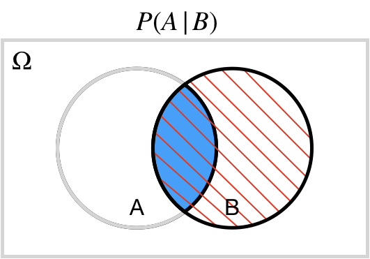 ]
---
## Subset: $A \subseteq \Omega$
$A \subseteq \Omega$: $A$ is a *subset* of $\Omega$.
$A \subset \Omega$: $A$ is a *proper subset* of $\Omega$.
.center[
]
---
## Subset: $A \subseteq \Omega$
$A \subseteq \Omega$: $A$ is a *subset* of $\Omega$.
$A \subset \Omega$: $A$ is a *proper subset* of $\Omega$.
.center[ ]
---
## Superset: $\Omega \supseteq A$
$\Omega \supseteq A$: $A$ is a *superset* of $\Omega$.
$\Omega \supset A$: $A$ is a *proper superset* of $\Omega$.
.center[
]
---
## Superset: $\Omega \supseteq A$
$\Omega \supseteq A$: $A$ is a *superset* of $\Omega$.
$\Omega \supset A$: $A$ is a *proper superset* of $\Omega$.
.center[ ]
---
## Element of: $X \in A$
$X \in A$: $X$ is an *element of* $A$.
.center[
]
---
## Element of: $X \in A$
$X \in A$: $X$ is an *element of* $A$.
.center[ ]
---
## Empty set: $\varnothing$
$A\cap E = \varnothing$: the intersection of $A$ and $E$ is the empty set.
.center[
]
---
## Empty set: $\varnothing$
$A\cap E = \varnothing$: the intersection of $A$ and $E$ is the empty set.
.center[ ]
---
layout: false
# Identities of Probability
* The probability of $A^c$ is $1$ minus the probability of $A$:
* $P(A^c) = 1-P(A)$.
* If $A$ is a subset of $B$, then the probability of $A$ is less than or equal to the probability of $B$:
* $A \subseteq B \implies P(A)\leq P(B)$.
* The probability of a union is equal to the sum of the probabilities minus the probability of an intersection:
* $P(A \cup B) = P(A) + P(B) - P(A\cap B)$.
---
# De Morgan's Laws
* Complement of the union is equal to the intersection of the complements.
.center[
]
---
layout: false
# Identities of Probability
* The probability of $A^c$ is $1$ minus the probability of $A$:
* $P(A^c) = 1-P(A)$.
* If $A$ is a subset of $B$, then the probability of $A$ is less than or equal to the probability of $B$:
* $A \subseteq B \implies P(A)\leq P(B)$.
* The probability of a union is equal to the sum of the probabilities minus the probability of an intersection:
* $P(A \cup B) = P(A) + P(B) - P(A\cap B)$.
---
# De Morgan's Laws
* Complement of the union is equal to the intersection of the complements.
.center[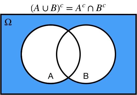 ]
---
# De Morgan's Laws
* Complement of the intersection is equal to the union of the complements.
.center[
]
---
# De Morgan's Laws
* Complement of the intersection is equal to the union of the complements.
.center[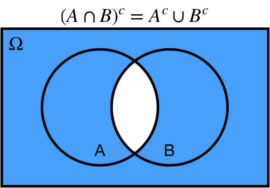 ]
---
# De Morgan's Laws
1. Complement of the union is equal to the intersection of the complements:
* $(A \cup B)^c = A^c \cap B^c$.
2. Complement of the intersection is equal to the union of the complements:
* $(A \cap B)^c = A^c \cup B^c$.
.center[ ]
---
# Independence
We say that two events $A$ and $B$ are independent, $A\perp \!\!\! \perp B$, *if and only if* one of the followings hold true:
* $P(A \cap B) = P(A) P(B)$;
* $P(A|B) = P(A)$;
* $P(B|A) = P(B)$.
This is an *extremely* important concept in statistics!
---
# Conditional Probability
The conditional probability of $A$ given $B$ is equal to the joint probability of $A$ and $B$ divided by the marginal probability of $B$:
$$P(A|B) = \dfrac{P(A\cap B)}{P(B)}.$$
Note that this implies
$$P(A\cap B) = P(A|B) P(B).$$
---
# Bayes' Rule
$$P(A|B) = \dfrac{P(A\cap B)}{P(B)}$$
also implies
$$P(A|B) = \dfrac{P(B|A)P(A)}{P(B)},$$
which is commonly known as **Bayes' rule**!
We won't get into the details in this class, but this can be a very useful result for reversing the conditions in our analysis.
For example: There is a big difference between the probability of having a disease given a positive screening, and the probability of a positive screening given a disease! These concepts are often confused in popular media!
---
# Law of Total Probability
We say that a set of events is a **partition** if all the followings hold:
* The set does not contain the empty set;
* The union of the events in the set is equal to the sample space;
* The intersection of any two distinct events in the set is equal to the empty set.
Note that an event and its complement always define a partition!
.center[
]
---
# De Morgan's Laws
1. Complement of the union is equal to the intersection of the complements:
* $(A \cup B)^c = A^c \cap B^c$.
2. Complement of the intersection is equal to the union of the complements:
* $(A \cap B)^c = A^c \cup B^c$.
.center[ ]
---
# Independence
We say that two events $A$ and $B$ are independent, $A\perp \!\!\! \perp B$, *if and only if* one of the followings hold true:
* $P(A \cap B) = P(A) P(B)$;
* $P(A|B) = P(A)$;
* $P(B|A) = P(B)$.
This is an *extremely* important concept in statistics!
---
# Conditional Probability
The conditional probability of $A$ given $B$ is equal to the joint probability of $A$ and $B$ divided by the marginal probability of $B$:
$$P(A|B) = \dfrac{P(A\cap B)}{P(B)}.$$
Note that this implies
$$P(A\cap B) = P(A|B) P(B).$$
---
# Bayes' Rule
$$P(A|B) = \dfrac{P(A\cap B)}{P(B)}$$
also implies
$$P(A|B) = \dfrac{P(B|A)P(A)}{P(B)},$$
which is commonly known as **Bayes' rule**!
We won't get into the details in this class, but this can be a very useful result for reversing the conditions in our analysis.
For example: There is a big difference between the probability of having a disease given a positive screening, and the probability of a positive screening given a disease! These concepts are often confused in popular media!
---
# Law of Total Probability
We say that a set of events is a **partition** if all the followings hold:
* The set does not contain the empty set;
* The union of the events in the set is equal to the sample space;
* The intersection of any two distinct events in the set is equal to the empty set.
Note that an event and its complement always define a partition!
.center[ ]
---
# Law of Total Probability
The **law of total probability** states that given a partition $P_1, P_2, \ldots, P_n$, then
$$P(A) = P(A|P_1)P(P_1) + P(A|P_2)P(P_2) + \cdots + P(A|P_n)P(P_n).$$
Commonly, our partition is some event $B$ and its complement:
$$P(A) = P(A|B)P(B) + P(A|B^c)P(B^c).$$
.center[
]
---
# Law of Total Probability
The **law of total probability** states that given a partition $P_1, P_2, \ldots, P_n$, then
$$P(A) = P(A|P_1)P(P_1) + P(A|P_2)P(P_2) + \cdots + P(A|P_n)P(P_n).$$
Commonly, our partition is some event $B$ and its complement:
$$P(A) = P(A|B)P(B) + P(A|B^c)P(B^c).$$
.center[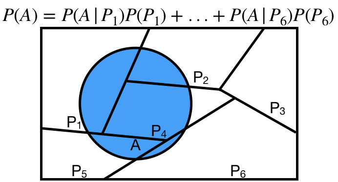 ]
---
class: inverse
# Appendix B. Random Variables
---
# Random Variables
Typically, we don't care about specific events occuring.
Instead, we tend to focus on functions of our events.
These functions are called **random variables**.
More formally1, a random variable $X$ can be defined as function $X: \Omega \mapsto \mathbb{R}$. For example,
* the number of heads out of 10 coin flips;
* the sum of 8 standard die rolls;
* the average value of 1,000 simulations from a $\mathcal{N}(0,1)$.
Typically, a random variable is denoted by a uppercase letter, such as $X$, and values that the random variable takes is denoted by a lowercase letter, such as $x$.
For example, we might ask the $P(X=x)$ for multiple values of $x$.
We call the set of all values a random variable can take the **support** of that random variable.
.footnote[[1] It is still not very formal.]
---
# Random Variables
Random variables are **not** events!
This can be confusing because often use similar notation with random variables and events. Think of an event as an outcome that can lead to a certain value of a random variable. For example,
* Event in 10 coinflips: $\{THHTTTHTTH\}$.
* Random variable representing the number of heads $X = 4$.
* Event in 8 standard die rolls: $\{2, 4, 2, 1, 5, 4, 2, 6\}$.
* Random variable representing the sum $X = 25$.
---
# Discrete Random Variables
Random variables are **discrete** if there are a finite1 number of values in the support.
We've already seen some examples of this in class from the binomial distribution!
We define the **probability mass function**, or **PMF**, of a discrete random variable $X \sim Bin(n,p)$ as
$$P(X=k|n,p) = \begin{pmatrix} n\\ k\end{pmatrix} p^k(1-p)^{n-k}$$
Probability mass functions must satisfy:
1. $0 \leq P(X=x) \leq 1$ for all $x$
2. $\sum_{x \in support(X)} P(X = x) = 1$
3. For any set $A\subseteq support(X)$, $P(X \in A) = \sum_{x \in A} P(X = x)$
.footnote[[1] or countably infinite]
---
# Continuous Random Variables
Random variables are **continuous** if the support is uncountably infinite.
We've already seen some examples of this in class from the normal distribution!
We define the **probability density function**, or **PDF** of a continuous random variable $X \sim \mathcal{N}(\mu, \sigma^2)$ as
$$f_X(x) = \dfrac{1}{\sqrt{2\pi\sigma^2}} e^{-\dfrac{1}{2}\left(\dfrac{x-\mu}{\sigma}\right)^2}$$
Probability density functions must satisfy:
1. $f_X(x) > 0$ for all $x \in support(X)$;
2. The area under the curve of the pdf in the support is equal to $1$. That is,
$\int_{support(X)} f_X(x)dx = 1$;
3. If $A$ is some interval in the support of $X$, then $P(X \in A) = \int_A f_X(x)dx$.
Note that the second and third properties are essentially the continuous versions of the corresponding properties of discrete PMFs!
---
# Expected Value
The **expected value** or expectation of a random variable, denoted $E[X]$ or $\mathbb{E}[X]$, is the mean of the random variable.
Intuitively, it can be thought of as a weighted average of all values in the support, weighted by their value in the pdf/pmf.
Expected values satisfy the following properties for random variables $X$, $Y$ and constants $a$, $b$:
* $\mathbb{E}[a] = a$;
* $\mathbb{E}[aX + b] = a \cdot \mathbb{E}[X] + b$;
* $\mathbb{E}[X + Y] = \mathbb{E}[X] + \mathbb{E}[Y]$.
If $X$ and $Y$ are independent, then
* $\mathbb{E}[XY] = \mathbb{E}[X]\cdot \mathbb{E}[Y]$.
---
# Variance
The **variance** of a random variable is the expected squared difference between a random variable and its mean.
$$\text{Var}(X)=\mathbb{E}[(X - \mathbb{E}[X])^2].$$
Intuitively, this measures how far the values of $X$ are from their mean, on average.
It is a measure of spread, or variability.
Variances satisfy the following properties for a random variable $X$ and constants $a, b$:
* $\text{Var}(a) = 0$
* $\text{Var}(aX + b) = a^2\cdot \text{Var}(X)$
The square root of the variance is known as the **standard deviation**, because it is the expected (standard) magnitude of the difference (deviation) between a random variable and its mean.
More detailed review of the basic probability theory can be found in Section 3 of [this notes](https://zhangyk8.github.io/teaching/file_stat548/CS547_Proof_Probability_new.pdf).
]
---
class: inverse
# Appendix B. Random Variables
---
# Random Variables
Typically, we don't care about specific events occuring.
Instead, we tend to focus on functions of our events.
These functions are called **random variables**.
More formally1, a random variable $X$ can be defined as function $X: \Omega \mapsto \mathbb{R}$. For example,
* the number of heads out of 10 coin flips;
* the sum of 8 standard die rolls;
* the average value of 1,000 simulations from a $\mathcal{N}(0,1)$.
Typically, a random variable is denoted by a uppercase letter, such as $X$, and values that the random variable takes is denoted by a lowercase letter, such as $x$.
For example, we might ask the $P(X=x)$ for multiple values of $x$.
We call the set of all values a random variable can take the **support** of that random variable.
.footnote[[1] It is still not very formal.]
---
# Random Variables
Random variables are **not** events!
This can be confusing because often use similar notation with random variables and events. Think of an event as an outcome that can lead to a certain value of a random variable. For example,
* Event in 10 coinflips: $\{THHTTTHTTH\}$.
* Random variable representing the number of heads $X = 4$.
* Event in 8 standard die rolls: $\{2, 4, 2, 1, 5, 4, 2, 6\}$.
* Random variable representing the sum $X = 25$.
---
# Discrete Random Variables
Random variables are **discrete** if there are a finite1 number of values in the support.
We've already seen some examples of this in class from the binomial distribution!
We define the **probability mass function**, or **PMF**, of a discrete random variable $X \sim Bin(n,p)$ as
$$P(X=k|n,p) = \begin{pmatrix} n\\ k\end{pmatrix} p^k(1-p)^{n-k}$$
Probability mass functions must satisfy:
1. $0 \leq P(X=x) \leq 1$ for all $x$
2. $\sum_{x \in support(X)} P(X = x) = 1$
3. For any set $A\subseteq support(X)$, $P(X \in A) = \sum_{x \in A} P(X = x)$
.footnote[[1] or countably infinite]
---
# Continuous Random Variables
Random variables are **continuous** if the support is uncountably infinite.
We've already seen some examples of this in class from the normal distribution!
We define the **probability density function**, or **PDF** of a continuous random variable $X \sim \mathcal{N}(\mu, \sigma^2)$ as
$$f_X(x) = \dfrac{1}{\sqrt{2\pi\sigma^2}} e^{-\dfrac{1}{2}\left(\dfrac{x-\mu}{\sigma}\right)^2}$$
Probability density functions must satisfy:
1. $f_X(x) > 0$ for all $x \in support(X)$;
2. The area under the curve of the pdf in the support is equal to $1$. That is,
$\int_{support(X)} f_X(x)dx = 1$;
3. If $A$ is some interval in the support of $X$, then $P(X \in A) = \int_A f_X(x)dx$.
Note that the second and third properties are essentially the continuous versions of the corresponding properties of discrete PMFs!
---
# Expected Value
The **expected value** or expectation of a random variable, denoted $E[X]$ or $\mathbb{E}[X]$, is the mean of the random variable.
Intuitively, it can be thought of as a weighted average of all values in the support, weighted by their value in the pdf/pmf.
Expected values satisfy the following properties for random variables $X$, $Y$ and constants $a$, $b$:
* $\mathbb{E}[a] = a$;
* $\mathbb{E}[aX + b] = a \cdot \mathbb{E}[X] + b$;
* $\mathbb{E}[X + Y] = \mathbb{E}[X] + \mathbb{E}[Y]$.
If $X$ and $Y$ are independent, then
* $\mathbb{E}[XY] = \mathbb{E}[X]\cdot \mathbb{E}[Y]$.
---
# Variance
The **variance** of a random variable is the expected squared difference between a random variable and its mean.
$$\text{Var}(X)=\mathbb{E}[(X - \mathbb{E}[X])^2].$$
Intuitively, this measures how far the values of $X$ are from their mean, on average.
It is a measure of spread, or variability.
Variances satisfy the following properties for a random variable $X$ and constants $a, b$:
* $\text{Var}(a) = 0$
* $\text{Var}(aX + b) = a^2\cdot \text{Var}(X)$
The square root of the variance is known as the **standard deviation**, because it is the expected (standard) magnitude of the difference (deviation) between a random variable and its mean.
More detailed review of the basic probability theory can be found in Section 3 of [this notes](https://zhangyk8.github.io/teaching/file_stat548/CS547_Proof_Probability_new.pdf).