---
title: "STAT 302 Statistical Computing"
subtitle: "Lecture 6: Simulations"
author: "Yikun Zhang (_Winter 2024_)"
date: ""
output:
  xaringan::moon_reader:
    css: ["uw.css", "fonts.css"]
    lib_dir: libs
    nature:
      highlightStyle: tomorrow-night-bright
      highlightLines: true
      countIncrementalSlides: false
      titleSlideClass: ["center","top"]
---

```{r setup, include=FALSE, purl=FALSE}
options(htmltools.dir.version = FALSE)
knitr::opts_chunk$set(comment = "##")
library(kableExtra)
```

# Outline

1. Simulation Basics

2. Pseudo-Randomness and Seeds

3. Simulation Tools in R

4. Integral Approximation via Monte Carlo Methods

5. Distribution Estimation and Sampling via Monte Carlo Methods

6. Bootstrapping

7. Ad hoc Network (Final Project)

<font size="4">* Acknowledgement: Parts of the slides are modified from the course materials by Prof. Ryan Tibshirani, Prof. Yen-Chi Chen, Prof. Alexander Giessing, Prof. Deborah Nolan, and Prof. Noureddine El Karoui. </font>

---
class: inverse

# Part 1: Simulation Basics

---

# What is Simulation?

- A simulation imitates the operation of real-world processes or systems with the use of a computer software. 

--

  - In most cases, simulation involves creating data by (pseudo-)random number generators and using that data to study a problem of interest.
  
  - Such simulation process is also known as the [Monte Carlo Methods](https://en.wikipedia.org/wiki/Monte_Carlo_method), whose name originates from the Monte Carlo Casino in Monaco.
  
--
  
Can you think of any examples from this or other classes when you have used simulations to answer a question? 

---

# An Example of Simulation in Cosmology

<p align="center">
<img src="./figures/illustris_z0.png" width="400"/>
</p>
<p align="center">
Exterior view of the dark matter density distribution in the full simulation box at redshift zero for <a href="https://www.illustris-project.org/">Illustris Simulation Project</a>.
</p>

---

# Why Do We Need Simulations?

To answer some scientific questions, we often need data evidence and experimental results to support our findings.

--

- However, observational data are generally expensive to obtain.

--

- On the contrary, it is relatively at a lower cost to generate synthetic data and implement a computer programming to conduct experiments.

- In addition, simulations sometimes can be easier and more realistic than hand calculations.

---

# Concrete Motivations for Simulations

A well-designed simulation can provide a solid estimator to statistical quantities and their uncertainty measures that are analytically difficult to obtain the exact answer.

--

- What is the probability of flipping 10 fair coins and getting 9 heads and 1 tails?

  - We can compute by hand as ${10 \choose 9} \left(\frac{1}{2}\right)^9 \left(1-\frac{1}{2}\right) \approx 0.0097656$.
  
--
  
  - Nevertheless, the simulation-based approximation could be more convenient.
  
```{r}
set.seed(123)
coins = rbinom(n = 5000000, size = 10, prob = 0.5)
mean(coins == 9)
```

---

# Concrete Motivations for Simulations

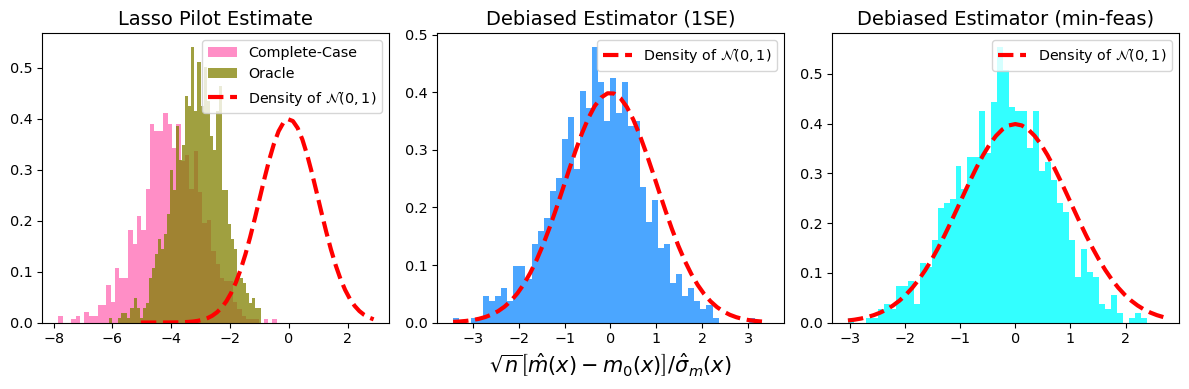
It also helps evaluate the performance of our proposed statistical method, such as its asymptotic normality and time efficiency.

<p align="center">
<img src="./figures/cirsym_lasso_bias_expl_x4_beta1.png" alt="lasso" width="550"/>
</p>

--

Simulation can also lead to a more efficient hypothesis testing or other statistical procedures than the original one.

  - Example: The Monte Carlo alternative to the [permutation test](https://en.wikipedia.org/wiki/Permutation_test).

---

# Concrete Motivations for Simulations
  
Simulation also provides a feasible way to generate random samples from a "partially known" probability distribution.

<p align="center">
<img src="./figures/rejectionsampling.png" width="550"/>
</p>
<p align="center">
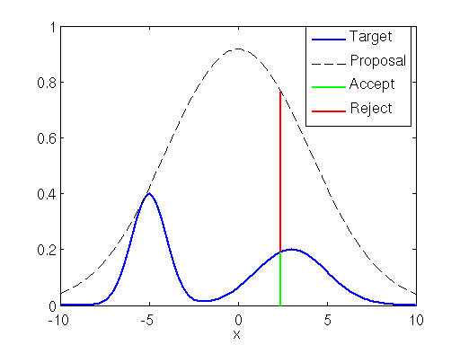
<font size="5"> <a href="https://en.wikipedia.org/wiki/Rejection_sampling">Acceptance-Rejection Sampling</a></font>
</p>

---

# Concrete Motivations for Simulations

Does simulation only appear in Statistics? Can other fields benefit from the usage of simulation?

--

- Monte Carlo methods have been developed into a technique called [Monte Carlo tree search](https://en.wikipedia.org/wiki/Monte_Carlo_tree_search) that is useful for searching for the best move in a game.

<p align="center">
<img src="./figures/MCTS_Algorithm.png" width="800"/>
</p>

- The Monte Carlo tree search has been successfully combined with deep neural networks to tackle the multiple board games, such as Go, Chess, Texas hold 'em, etc. See the introduction to [AlphaGo](https://www.deepmind.com/research/highlighted-research/alphago).

---

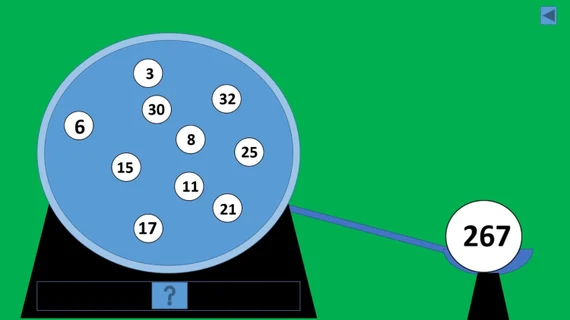
# Overview of Monte Carlo Simulations

A typical Monte Carlo simulation often follows a procedure as below.

1. Define a domain of possible inputs.

2. Generate inputs randomly from a probability distribution over the domain.

3. Perform a deterministic computation on the inputs.

4. Aggregate the results.

Do you know what the first known Monte Carlo simulation is?

--

<p align="center">
<img src="./figures/Buffon_needle.png" width="300"/>
</p>
<p align="center">
<font size="4"> <a href="https://en.wikipedia.org/wiki/Buffon%27s_needle_problem">Buffon's Needle Problem</a> for Estimating $\pi$</font>
</p>

---

# An Example of Monte Carlo Simulation

```{r}
set.seed(123)
n = 400000
x = runif(n, min = 0, max = 1)
y = runif(n, min = 0, max = 1)
mean(x^2 + y^2 < 1) * 4
```

<p align="center">
<img src="./figures/Pi_30K.gif" width="380"/>
</p>

---
class: inverse

# Part 2: Pseudo-Randomness and Seeds

---

# Random Number Generation in R

Most of the simulations require us to generate some random observations from a probability distribution.

--

Recall from Lab 2 that we have the utility functions:

- `rnorm()`: generates the normally distributed random variables/observations.

- `rbinom()`: generates the random variables/observations from a binomial distribution.

We can replace "norm" or "binom" with the name of another distribution, and the same function applies, e.g., "t", "unif", "exp", "gamma", "chisq", "pois", etc. 

---

# How Does R Generate Random Numbers?

There are no computer software that can generate completely random numbers, neither did R.

--

Instead, R uses a **pseudo-random number generator**:

- It starts with a **seed** and an **algorithm** (i.e., a function).

- The **seed** is input into the algorithm, and a (pseudo-random) number is returned. This number is then plugged into the algorithm, and the next (pseudo-random) number is created.

- The **algorithm** guarantees that the output numbers behave like random values.

---

# Linear Congruential Generator

One example of such an algorithm is the **Linear Congruential Generator**, which uses modular arithmetic to generate "random" numbers:

- Based on two parameters $m$ and $b$ and the initial value $x_0$ (i.e., the seed), the first "random number" $x_1$ is generated as follows:
$$x_1 = b \cdot x_0 \mod m.$$
- The subsequent numbers are generated recursively,
$$x_{n+1} = b \cdot x_n \mod m$$
for $n=1,2,...$.

---

# Linear Congruential Generator (Small $m$)

```{r fig.align='center', fig.height=5}
LinCongGen = function(n, seed, m = 64, b = 3){
  pseudo_num = numeric(n+1)
  pseudo_num[1] = seed
  for(i in 1:n){
    pseudo_num[i+1] = (pseudo_num[i]*b) %% m
  }
  return(pseudo_num[2:(n+1)])
}
n = 1000
seed = 17
rand_num = LinCongGen(n, seed, m = 64, b = 3)
plot(c(seed, rand_num[1:(n-1)]), rand_num, xlab = "Input Numbers", ylab = "Output Numbers")
```

---

# Linear Congruential Generator (Large $m$)


```{r fig.align='center', fig.height=5}
n = 1000
seed = 17
rand_num = LinCongGen(n, seed, m = 2^32, b = 3)
plot(c(seed, rand_num[1:(n-1)]), rand_num, xlab = "Input Numbers", ylab = "Output Numbers")
```

The output numbers are still not "random" enough.

---

# Linear Congruential Generator (Large $m$, Large $b$)


```{r fig.align='center', fig.height=5.5}
n = 1000
seed = 17
rand_num = LinCongGen(n, seed, m = 2^32, b = 69069)
plot(c(seed, rand_num[1:(n-1)]), rand_num, xlab = "Input Numbers", ylab = "Output Numbers")
```

---

# Pseudo-Random Number Generator in R

- Studying algorithms of generating more "random" numbers is an interesting research area in its own right.

--

- The default algorithm in R (and in nearly all software languages) is called the "Mersenne-Twister" algorithm.

- Type `?Random` in our R console to read more about this (and to read how to change the algorithm used for the pseudo-random number generation, which we should never really have to do that).

<p align="center">
<img src="./figures/random_number.webp" width="400"/>
</p>

---

# An Important Role of the "Seed"

One of the biggest advantages of pseudo-random number generators is that we can have some controls over the simulation results by setting the **seed** beforehand.

--

- The seed is just an integer, and can be set with `set.seed()`.

- It is very important to set our seed in the **proper** location of our code to make our simulation results _valid_ and _reproducible_.

<p align="center">
<img src="./figures/reproduce.png" width="600"/>
</p>

---

# Demonstrations of `set.seed()`

If we don't set the seed, it is not surprising to see different draws each time we call any random number generating functions.

```{r}
mean(rnorm(6))

mean(rnorm(6))
```

--

```{r}
set.seed(123)
mean(rnorm(6))

set.seed((123))
mean(rnorm(6))
```

---

# Demonstrations of `set.seed()`

Each time the seed is set, the same sequence follows (indefinitely).

```{r}
set.seed(123)
rnorm(3); rnorm(2); rnorm(1)
```

```{r}
set.seed(123)
rnorm(3); rnorm(2); rnorm(1)
```


---
class: inverse

# Part 3: Simulation Tools in R

---

# `sample()` Function

The `sample()` function takes a sample of the pre-specified size from the elements of `x` using either with or without replacement.

```{r}
sample(letters, size = 10, replace = FALSE, prob = NULL)
```

--

We can make the sampling results reproducible by setting the seed.

```{r}
set.seed(123)
sample(letters, size = 10, replace = FALSE, prob = NULL)
```

---

# Betting Red in Roulette

What is the chance that a spin of the Roulette wheel lands on red?

<p align="center">
<img src="./figures/American_roulette.webp" width="750"/>
</p>

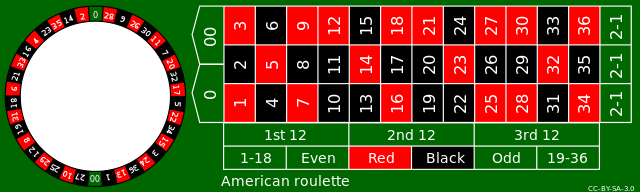
- There are 38 pockets in the Roulette wheel:
  
  - 18 blacks, 18 reds, and 2 greens.

--

- We can estimate the chance by simulating the Roulette wheel many, many, many times via the `sample()` function in R:
$$\frac{\# \text{ reds}}{\# \text{ draws}} \approx \text{Chance of reds}.$$

---

# Betting Red in Roulette

What is the chance that a spin of the Roulette wheel lands on red?

```{r}
rou_vec = c(rep(c("black", "red"), each = 18), rep("green", 2))

set.seed(123)
samp_res = sample(rou_vec, size = 10000, replace = TRUE)
mean(samp_res == "red")
cat("The estimation error is ", abs(mean(samp_res == "red") - 18/38), ".", sep = "")
```

---

# Betting Red in Roulette

As the number of draws increases, the proportions of reds becomes closer to the true probability $\frac{18}{38}$.

```{r}
set.seed(123)
samp_res = sample(rou_vec, size = 1000000, replace = TRUE)
cat("The estimation error is ", abs(mean(samp_res == "red") - 18/38), ".", sep = "")
```

--

This reveals the principle of **Law of Large Numbers** in Statistics:
$$\frac{1}{n} \sum_{i=1}^n X_i \to p \quad \text{ in probability } \quad \text{or even} \quad \text{ almost surely},$$
where $p$ is the probability of lands on reds in the Roulette wheel, and 
$$
X_i = 
\begin{cases}
1 & \text{ when landing on reds for the i-th draw},\\
0 & \text{ when landing on other colors for the i-th draw}.\\
\end{cases}
$$

---

# Betting Red in Roulette

By increasing the sample size, the precision of the estimated probability of the Roulette wheel landing on reds can be improved.

- However, for any fixed sample size $n$, what are the typical deviations (or standard errors) from the average of these sample proportions of reds?

--

  - To quantify these deviations (or standard errors), we need to repeat the previous sampling procedure $B$ times, where $B$ is sufficiently large.
  
  - In R, such repetitions can be handled by the `replicate()` function.

---

# `replicate()` Function

Let's fix the sample size $n$ to be 10000 and repeat the entire procedure of estimating the probability of the Roulette wheel landing on reds $B=3000$ times.

```{r}
set.seed(123)   ## We should set the seed here!!
rep_means = replicate(3000, 
                      mean(sample(rou_vec, size = 10000, replace = TRUE) == "red"))
```

Note: The `replicate` function is a wrapper for the common use of `sapply()` for repeated evaluation of an expression.

--

```{r}
set.seed(123)   ## We should set the seed here!!
rep_means2 = replicate(3000, {
  samp_res = sample(rou_vec, size = 10000, replace = TRUE)
  mean(samp_res == "red")
})
all.equal(rep_means, rep_means2)
```

---

# Distribution of the Sample Proportions

```{r fig.align='center', fig.width=7, fig.height=6}
hist(rep_means, breaks = 30, freq = FALSE, xlab = "Sample Proportion of Reds", 
     main = "Histogram of the Sample Proportions")
```

---

# Rate of Convergence of the Sample Proportions

How quickly do the sample proportions approach the true probability $\frac{18}{38}$ as the sample size $n$ increases?

--

<p align="center">
<img src="./figures/Red_decay.png" width="650"/>
</p>

Note: The red curves plot the trends $\pm \sqrt{\frac{p(1-p)}{n}}$.

---

# Distribution of the Sample Proportions

```{r fig.align='center', fig.width=7, fig.height=5, echo=FALSE}
hist(rep_means, breaks = 30, freq = FALSE, xlab = "Sample Proportion of Reds", 
     main = "Histogram of the Sample Proportions")
```

- The distribution of the sample proportions of reds looks roughly like the normal distribution with

  - Center: `mean`(sample proportions) $\approx \frac{18}{38}$.
  
  - Spread: `sd`(sample proportions) $\approx \sqrt{\frac{p(1-p)}{n}}$.
  
---

# Distribution of the Sample Proportions

```{r fig.align='center', fig.width=7, fig.height=5, echo=FALSE}
hist(rep_means, breaks = 30, freq = FALSE, xlab = "Sample Proportion of Reds", 
     main = "Histogram of the Sample Proportions")
```

This reveals the **Central Limit Theorem** in Statistics:
$$\frac{\sqrt{n} (\bar{X}_n - p) }{\sqrt{p(1-p)}} \to N(0,1) \quad \text{ in distribution},$$
where $\bar{X}_n = \frac{1}{n} \sum_{i=1}^n X_i$.

---

# Simulation Example: Drug Effect Model

Suppose that we had a model to quantify how a drug will reduce the tumor size of a patient in percentage.

--

- A patient who was not given the drug experiences the reduction of tumor size in percentage as:
$$X_{\text{no drug}} \sim 100 \cdot \text{Exponential}(\text{mean}=R), \quad R\sim \text{Uniform}(0,1).$$

- A patient who was given the drug experiences a reduction of tumor size in percentage as:
$$X_{\text{drug}} \sim 100 \cdot \text{Exponential}(\text{mean}=2).$$

Note: Here, $\text{Exponential}(\text{mean}=\lambda)$ stands for the exponential distribution whose mean is $\lambda$, and $\text{Uniform}$ denotes the uniform distribution.

---

# Simulation Example: Drug Effect Model

Given such a drug effect model, our scientist collaborators ask us: 

- How many patients would we need to have in each group (_drug_ or _no drug_) in order to reliably see that the average reduction in tumor size is large?

This question can be answered by complicated calculations or the _simulation_ methods that we learned.

--

```{r}
# Simulate, supposing 60 subjects in each group 
set.seed(123)
n = 60 
mu_drug = 2
mu_nodrug = runif(n, min = 0, max = 1)
x_drug = 100*rexp(n, rate = 1/mu_drug) 
x_nodrug = 100*rexp(n, rate = 1/mu_nodrug)
```

---

# Simulation Example: Drug Effect Model

```{r fig.align='center', eval=FALSE}
# Find the range of all the measurements together
x_range = range(c(x_nodrug, x_drug))
breaks = seq(min(x_range), max(x_range), length=20)

# Overlaid the histograms of no drug and drug measurements
hist(x_nodrug, breaks = breaks, probability=TRUE, xlim = x_range, col = "lightgray", xlab = "Percentage reduction in tumor size", main = "Comparison of tumor reduction")
hist(x_drug, breaks = breaks, probability = TRUE, col = rgb(1,0,0,0.2), add = TRUE) 

# Draw estimated densities on top
lines(density(x_nodrug), lwd=3, col=1)
lines(density(x_drug), lwd=3, col=2)
legend("topright", legend=c("No drug","Drug"), lty=1, lwd=3, col=1:2)
```

---

# Simulation Example: Drug Effect Model

```{r fig.align='center', echo=FALSE}
# Find the range of all the measurements together
x_range = range(c(x_nodrug, x_drug))
breaks = seq(min(x_range), max(x_range), length=20)

# Overlaid the histograms of no drug and drug measurements
hist(x_nodrug, breaks = breaks, probability=TRUE, xlim = x_range, col = "lightgray", xlab = "Percentage reduction in tumor size", main = "Comparison of tumor reduction")
hist(x_drug, breaks = breaks, probability = TRUE, col = rgb(1,0,0,0.2), add = TRUE) 

# Draw estimated densities on top
lines(density(x_nodrug), lwd=3, col=1)
lines(density(x_drug), lwd=3, col=2)
legend("topright", legend=c("No drug","Drug"), lty=1, lwd=3, col=1:2, cex = 1.5)
```

---

# Simulation Example: Drug Effect Model

A single simulation is generally not trustworthy, and we need to repeat the above simulation for many times. Here is a guideline:

1. Write a function to complete a single run of our simulation.

2. Set the seed to ensure reproducibility.

3. Use an iteration (via `replicate()` function) to run our simulation over and over again.

4. Save our simulation result as in `.rdata` or other format files.

We will revisit this drug effect model example in Lab 6.

---
class: inverse

# Part 4: Integral Approximation via Monte Carlo Methods

---

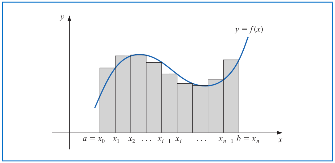
# Integration

The Riemann integral of the function $f$ on the interval $[a,b]$ is the following limit, provided it exists:
$$\int_a^b f(x) dx = \lim_{\max \Delta x_i \to 0} \sum_{i=1}^n f(z_i) \Delta x_i,$$
where the numbers $x_0,x_1,...,x_n$ satisfy $a=x_0\leq x_1 \leq \cdots \leq x_n=b$, where $\Delta x_i = x_i-x_{i-1}$ for each $i=1,2,...,n$ and $z_i$ is an arbitrary number in the interval $[x_{i-1}, x_i]$.

<p align="center">
<img src="./figures/riem_inte.png" width="600"/>
</p>

---

# Fundamental Theorem of Calculus

- If $f$ is a continuous function on $[a,b]$ and $F(x)=\int_a^x f(t) dt$, then $F'(x)=f(x)$ for any $x\in (a,b)$. Thus, $F$ is an anti-derivative of $f$.

--

- If $f$ is a continuous function on $[a,b]$  and $F$ is any anti-derivative of $f$, then 
$$\int_a^b f(x) dx = F(x)\Big|_{x=a}^b = F(b) - F(a).$$

<p align="center">
<img src="./figures/Fundamental_theorem_of_calculus.gif" width="420"/>
</p>

---

# Integral Approximation

Assume that we want to evaluate the following integral:
$$\int_0^1 e^{-x^3} dx.$$

--

- There are no analytic anti-derivative of the function $e^{-x^3}$.

- Traditionally, we will use the Riemann sum to approximate this integral as:
$$\sum_{j=1}^m e^{-z_j^3} \Delta x_j,$$
where the numbers $x_0,x_1,...,x_n$ satisfy $a=x_0\leq x_1\leq \cdots \leq x_n=b$ with $\Delta x_j = x_j-x_{j-1}, i=1,...,n$ and $z_j$ is arbitrarily chosen in the interval $[x_{j-1}, x_j]$.

---

# Monte Carlo Integration

The Monte Carlo method gives us an alternative approach to evaluate this integral $\int_0^1 e^{-x^3} dx$.

--

- Note that we can rewrite this integral as:
$$\int_0^1 e^{-x^3} dx = \int_0^1 e^{-x^3} \cdot 1 \,dx = \mathbb{E}\left(e^{-U^3} \right),$$
where $U$ is a $\text{Uniform}[0,1]$ distributed random variable.

- Hence, we can generate random samples $U_1,...,U_n \sim \text{Uniform}[0,1]$ and then compute that
$$\frac{1}{n} \sum_{i=1}^n e^{-U_j^3}.$$

---

# Monte Carlo Integration

- By Law of Large Number, we know that
$$\frac{1}{n} \sum_{i=1}^n e^{-U_j^3} \to \mathbb{E}\left(e^{-U_1^3}\right) = \int_0^1 e^{-x^3} dx.$$

```{r}
set.seed(123)
n = 100000
x = runif(n, min = 0, max = 1)
mean(exp(-x^3))
```


```{r}
inteFun1 = function(x) {
  exp(-x^3)
}
integrate(inteFun1, lower = 0, upper = 1)
```

---

# Importance Sampling

More generally, we consider evaluating the following quantity:
$$I = \mathbb{E}\left[g(X) \right] = \int g(x) \cdot p(x)\, dx,$$
where $g$ is a known function and $X$ is a random variable with density $p$.

--

We can approximate $I$ using a technique called **importance sampling**.

1. Pick a proposal density function (also called sampling density) $q$ from which we know how to generate random samples.

2. Generate random points $Y_1,...,Y_n$ from the proposal density $q$.

3. Then, the importance sampling estimator for $I$ is defined as:
$$\hat{I}_n = \frac{1}{n} \sum_{i=1}^n \frac{g(Y_i) \cdot p(Y_i)}{q(Y_i)}.$$

---

# Analysis on Importance Sampling

How good this importance sampling estimator is?

--

- $\hat{I}_n$ is an _unbiased_ estimator.
\begin{align*}
\text{Bias}\left(\hat{I}_n \right) &= \mathbb{E}\left(\hat{I}_n \right) - I\\
&= \mathbb{E}\left(\frac{g(Y_i) \cdot p(Y_i)}{q(Y_i)} \right) - I\\
&= \int \frac{g(y) \cdot p(y)}{q(y)} \cdot q(y) \, dy - I\\
&= \int g(y)\cdot p(y)\, dy - I =0.
\end{align*}

---

# Analysis on Importance Sampling

How good this importance sampling estimator is?

- The variance of $\hat{I}_n$ is
\begin{align*}
\text{Var}\left(\hat{I}_n \right) &= \frac{1}{n} \text{Var}\left[\frac{g(Y_i) \cdot p(Y_i)}{q(Y_i)} \right] \\
&= \frac{1}{n}\left\{\mathbb{E}\left[\frac{g^2(Y_i) \cdot p^2(Y_i)}{q^2(Y_i)} \right] - \underbrace{\mathbb{E}^2\left[\frac{g(Y_i) \cdot p(Y_i)}{q(Y_i)} \right]}_{I^2} \right\}\\
&= \frac{1}{n}\left[\int \frac{g^2(y) \cdot p^2(y)}{q(y)}\, dy - I^2  \right],
\end{align*}
which will converge to 0 as $n\to \infty$.

- Question: What will the optimal proposal density $q_{\text{opt}}$ be?
  
---

# Analysis on Importance Sampling

Question: What will the optimal proposal density $q_{\text{opt}}$ be?

- The optimal proposal density will be the one that minimizes the variance.

- Recall that Cauchy-Schwarz inequality is defined as:
$$\int A^2(y)\, dy \, \int B^2(y) \, dy \geq \left[\int A(y) B(y)\, dy \right]^2,$$
where $A(y)$ and $B(y)$ are two arbitrary functions and the equality holds when $A(y) \propto B(y)$.

---

# Analysis on Importance Sampling

Question: What will the optimal proposal density $q_{\text{opt}}$ be?

- Take $A^2(y) = \frac{g^2(y) \cdot p^2(y)}{q(y)}$ and $B^2(y)= q(y)$. Then, we have that
\begin{align*}
\int \frac{g^2(y) \cdot p^2(y)}{q(y)}\, dy &= \int \frac{g^2(y) \cdot p^2(y)}{q(y)}\, dy \cdot \underbrace{\int q(y)\, dy}_{=1} \\
&\geq \left[\int \frac{g(y) \cdot p(y)}{\sqrt{q(y)}} \cdot \sqrt{q(y)}\, dy \right]^2 \\
&= I^2.
\end{align*}

- It shows that the optimal proposal density $q_{\text{opt}}$ leads to 
$$\text{Var}\left(\hat{I}_{n,\text{opt}} \right) = \frac{1}{n} (I^2 -I^2) =0,$$
which is a **zero-variance** estimator!

---

# Analysis on Importance Sampling

Question: What will the optimal proposal density $q_{\text{opt}}$ be?

- The optimal proposal density $q_{\text{opt}}$ satisfies
$$\frac{g(y) \cdot p(y)}{\sqrt{q_{\text{opt}}(y)}} =A(y) \propto B(y) = \sqrt{q_{\text{opt}}(y)},$$
implying that 
$$q_{\text{opt}}(y) \propto g(y)\cdot p(y) \implies q_{\text{opt}}(y) = \frac{g(y)\cdot p(y)}{\int g(y)\cdot p(y)\, dy}.$$

--

- The above calculations tell us that the optimal proposal density $q_{\text{opt}}$ has 0 variance and it is unbiased. 

- Thus, we only need to sample from $q_{\text{opt}}$ once and will obtain the actual value of $I=\frac{g(Y_1) \cdot p(Y_1)}{q_{\text{opt}}(Y_1)}$ with $Y_1 \sim q_{\text{opt}}$.

---
class: inverse

# Part 5: Distribution Estimation and Sampling via Monte Carlo Methods

---

# Probability Distributions in Simulations

So far, the random numbers that we use in our simulations come from some well-known probability distributions, in which R provides some built-in functions to generate them.

- `rnorm()`, `rbinom()`, `rexp()`, `rt()`, `rgamma()`, `rchisq()`, `rpois()`, etc. See `?distributions` for details.

What if we don't have a built-in function for the probability distribution?

--

- If we only have the observed data $X_1,...,X_n$ from the target distribution and want to estimate the cumulative distribution function (CDF), we can consider using the empirical CDF (ECDF) and generate random samples from ECDF.

--

- If we know the density function $f$ (or an upper bound $M\geq \sup_x \frac{f(x)}{p(x)}$ with respect to some known density function $p$) and want to generate some random samples from $f$, we can consider using the **Acceptance-Rejection sampling**.

---

# Empirical CDF (ECDF)

Given the observed data $X_1,...,X_n$ from the target distribution, the ECDF is defined as:
$$\hat{F}_n(x) = \frac{1}{n} \sum_{i=1}^n I(X_i\leq x),$$
where $I: \mathbb{R} \to \{0,1\}$ is an indicator function.

```{r}
set.seed(123)
n = 600
z = rnorm(n, mean = 0, sd = 3)  # The observed data
x = seq(-3, 3, length = 100)
ecdf_fun = ecdf(z)
class(ecdf_fun)  # It is a function!
ecdf_fun(0)
```

---

# Empirical CDF (ECDF)

```{r fig.align='center', fig.height=6}
plot(x, ecdf_fun(x), lwd=2, col="red", type="l", ylab="CDF", main="ECDF")
lines(x, pnorm(x, mean = 0, sd = 3), lwd=2)
legend("topleft", legend=c("Empirical", "Actual"), lwd=2, col=c("red", "black"))
```

---

# Interlude: Kolmogorov-Smirnov Test

One application of ECDFs is the Kolmogorov-Smirnov test.

- The **Kolmogorov-Smirnoff (KS) statistic** is
$$\sqrt{\frac{n}{2}} \sup_{x} |F_n(x)-G_n(x)|,$$
where $F_n$ is the ECDF of $X_1,\ldots,X_n \sim F$ and $G_n$ is the ECDF of $Y_1,\ldots,Y_n \sim G$. 

--

- Under the null hypothesis $F=G$ (two distributions are the same), when $n \to \infty$, the KS statistic approaches the supremum of a Brownian bridge as:
$$\sup_{t \in [0,1]} |B(t)|,$$
where $B$ is a Gaussian process with $B(0)=B(1)=0$, mean $\mathbb{E}(B(t))=0$ for any $t\in [0,1]$, and covariance function $\mathrm{Cov}(B(s), B(t)) = \min\{s,t\} - st$ for any $t,s\in [0,1]$.

---

# Interlude: Kolmogorov-Smirnov Test

```{r fig.align='center', fig.height=6}
n = 500
t = 1:n/n
Sig = t %o% (1-t)
Sig = pmin(Sig, t(Sig))
eig = eigen(Sig)
Sig_half = eig$vec %*% diag(sqrt(eig$val)) %*% t(eig$vec)
B = Sig_half %*% rnorm(n)
plot(t, B, type="l")
```

---

# Interlude: Kolmogorov-Smirnov Test

Two facts about the Kolmogorov-Smirnov test:

1. It is *distribution-free*, meaning that the null distribution doesn't depend on $F$ and $G$!

--

2. If the null distribution is known, we can use one-sample Kolmogorov-Smirnov test. 

```{r}
ks.test(rnorm(n), rt(n, df = 1)) # Normal versus t1
ks.test(rnorm(n), "pt", df = 10) # Normal versus t10
```

---

# Acceptance-Rejection Sampling

Recall our example of estimating $\pi$:

<p align="center">
<img src="./figures/Pi_30K.gif" width="350"/>
</p>

--

- We sample points within the unit square and reject those points whose distances to the origin are larger than 1.

- Indeed, we already leverage the principle of Acceptance-Rejection sampling in this example.

---

# Acceptance-Rejection Sampling

Now, the density function $f$ is known, and we want to generate random samples from it.

1. We generate points uniformly from a larger region that includes the density function $f$.

2. Reject those points outside of the density region (red ones).

3. Keep the $x$-coordinates of the remaining points.

<p align="center">
<img src="./figures/rejection_sampling.png" width="320"/>
</p>

---

# Acceptance-Rejection Sampling

To utilize the previous Acceptance-Rejection sampling procedures, we need to know the rectangular region that encompasses the graph of the density function $f$.

--

- This rectangular region is hard to identify in most of cases.

- Instead, it is relatively easy to sample from some known density function $p$ and assess the supremum number $M \geq \sup_x \frac{f(x)}{p(x)}$ in advance.

- This leads to a more general Acceptance-Rejection sampling procedure.

---

# Acceptance-Rejection Sampling

A general/standard Acceptance-Rejection sampling procedure:

1. Choose a number $M \geq \sup_x \frac{f(x)}{p(x)}$ with respect to a proposal density $p$ from which we know how to draw samples.

  - For instance, $p$ can be the density function of $N(0,1)$.

2. Generate a random number $Y$ from the proposal density $p$ and another random number $U \sim \text{Uniform}[0,1]$.

3. If $U < \frac{f(Y)}{M \cdot p(Y)}$, accept $X=Y$ as a sampling point from $f$. Otherwise, go back to the previous step to draw a new pair of $(Y,U)$.

---

# Why Does Acceptance-Rejection Sampling Work?

Consider the CDF of an accepted sampling point $X$:
\begin{align*}
P(X\leq x) &= P(Y\leq x| \text{Accept } Y)\\
&= P\left(Y\leq x \Big| U < \frac{f(Y)}{M \cdot p(Y)} \right) \\
&= \frac{P\left(Y\leq x, U < \frac{f(Y)}{M \cdot p(Y)} \right)}{P\left(U < \frac{f(Y)}{M \cdot p(Y)} \right)}.
\end{align*}

We compute the numerator and denominator separately.

---

# Why Does Acceptance-Rejection Sampling Work?

For the numerator, we compute that 
\begin{align*}
&P\left(Y\leq x, U < \frac{f(Y)}{M \cdot p(Y)} \right)\\ 
&= \int P\left(Y\leq x, U < \frac{f(Y)}{M \cdot p(Y)} \Big| Y=y \right) \cdot p(y)\, dy\\
&= \int P\left(y\leq x, U < \frac{f(y)}{M \cdot p(y)} \right) \cdot p(y)\, dy\\
&= \int I(y\leq x) \cdot P\left(U < \frac{f(y)}{M \cdot p(y)} \right) \cdot p(y)\, dy\\
&= \int_{-\infty}^x \frac{f(y)}{M \cdot p(y)} \cdot p(y)\, dy\\
&= \frac{1}{M} \int_{-\infty}^x f(y)\, dy.
\end{align*}

---

# Why Does Acceptance-Rejection Sampling Work?

For the denominator, we compute that
\begin{align*}
P\left(U < \frac{f(Y)}{M \cdot p(Y)} \right) &= \int P\left(U < \frac{f(Y)}{M \cdot p(Y)} \Big| Y=y \right) \cdot p(y) \, dy\\
&= \int P\left(U < \frac{f(y)}{M \cdot p(y)} \right) \cdot p(y) \, dy\\
&= \int \frac{f(y)}{M \cdot p(y)} \cdot p(y) \, dy\\
&= \frac{1}{M} \int f(y)\, dy \\
&= \frac{1}{M}.
\end{align*}

---

# Why Does Acceptance-Rejection Sampling Work?

Combining the above results tells us that
\begin{align*}
P(X\leq x) &= \frac{P\left(Y\leq x, U < \frac{f(Y)}{M \cdot p(Y)} \right)}{P\left(U < \frac{f(Y)}{M \cdot p(Y)} \right)} \\
&= \frac{\frac{1}{M} \int_{-\infty}^x f(y)\, dy}{\frac{1}{M}} \\
&= \int_{-\infty}^x f(y)\, dy.
\end{align*}
This shows that the accepted sampling point $X$ does have its density function as $f$.

---

# Comments on Acceptance-Rejection Sampling

- We can generate random observations via the Acceptance-Rejection sampling from any density $f$ as long as we can evaluate $f$ at every point of its domain.

--

- However, if we don't choose $M \geq \sup_x \frac{f(x)}{p(x)}$, then the Acceptance-Rejection sampling can be very inefficient, i.e., we may reject a lot of realizations of $Y,U$ in order to accept a single realization of $X=Y$.

  - Recall that $P(\text{Accept } Y) = P\left(U < \frac{f(Y)}{M \cdot p(Y)} \right)=\frac{1}{M}$.
  
- More about the acceptance-rejection sampling can be found in [Notes 1](http://faculty.washington.edu/yenchic/19A_stat535/Lec9_MC.pdf) and [Notes 2](http://www.columbia.edu/~ks20/4703-Sigman/4703-07-Notes-ARM.pdf).

---
class: inverse

# Part 6: Bootstrapping

---

# Classical Problem in Statistics

Consider the scenario where we have a random sample $X_1,...,X_n$ and want to construct a statistic $T\equiv h(X_1,...,X_n)$ to estimate a population quantity $\theta$.

- $T\equiv h(X_1,...,X_n)$ is known as the _point estimate_ of $\theta$.

--

- Suppose that $X_1,...,X_n \sim P_{\theta}$ with $\theta$ being the mean/expectation. Then, the sample mean $T=\bar{X}_n=\frac{1}{n} \sum_{i=1}^n X_i$ is a natural estimator of the population mean $\theta$.

--

In many cases, however, we also want to quantify the uncertainty level for estimating $\theta$. This can be achieved by a $100\%\cdot (1-\alpha)$ confidence interval $[l, u]\equiv \left[l(X_1,...,X_n), u(X_1,...,X_n) \right]$, where $\alpha\in (0,1)$ and
$$\mathbb{P}\Big(\theta \in \left[l(X_1,...,X_n), u(X_1,...,X_n) \right] \Big) = 100\%\cdot (1-\alpha).$$

---

# Classical Asymptotic Theory

Suppose that $X_1,...,X_n \sim P_{\theta}$ with $\theta$ being the mean/expectation. Then, the sample mean $T=\bar{X}_n=\frac{1}{n} \sum_{i=1}^n X_i$ is a natural estimator of the population mean $\theta$.

- We can estimate the standard deviation as: 
$$\hat{\sigma}=\sqrt{\frac{1}{n-1}\sum_{i=1}^n (X_i-\bar{X}_n)^2}$$
and construct an asymptotic $100\%\cdot (1-\alpha)$ confidence interval for $\theta$ by the Central Limit Theorem as:
$$\left[\bar{X}_n - \frac{\hat{\sigma}}{\sqrt{n}} \cdot q_{1-\alpha/2},\; \bar{X}_n + \frac{\hat{\sigma}}{\sqrt{n}} \cdot q_{1-\alpha/2} \right],$$
where $q_{1-\alpha/2}$ is the $\left(1-\frac{\alpha}{2}\right)$ quantile of $\mathcal{N}(0,1)$.

---

# Limitations of the Asymptotic Theory

The validity of the preceding confidence interval $\left[\bar{X}_n - \frac{\hat{\sigma}}{\sqrt{n}} \cdot q_{1-\alpha/2},\; \bar{X}_n + \frac{\hat{\sigma}}{\sqrt{n}} \cdot q_{1-\alpha/2} \right]$ relies on two factors:

1. We know how to estimate the standard error $\frac{\sigma}{\sqrt{n}}$, i.e., the standard deviation of our statistic $T\equiv h(X_1,...,X_n)$.

2. The statistic $T\equiv h(X_1,...,X_n)$ takes the form $\bar{X}_n=\frac{1}{n} \sum_{i=1}^n X_i$, and we know its asymptotic/limiting distribution by the Central Limit Theorem.

--

**Questions:**

- What if the standard error has no closed-form expression or depends on too many unknown parameter?

- What if the statistic $T\equiv h(X_1,...,X_n)$ is a complicated function of $X_1,...,X_n$ that we have no ideas about its (limiting) distribution?

---

# The Bootstrap Principle

The above questions can be addressed by a computer-intensive procedure called the **bootstrap**.

- It was invented by [Professor Bradley Efron](https://en.wikipedia.org/wiki/Bradley_Efron) from Stanford University in 1979.

- It allows us to estimate the standard errors (and construct confidence intervals) without deriving the distribution of $T\equiv h(X_1,...,X_n)$.

--

**Bootstrap Principle:** Let $F$ be the CDF of the random sample $X_1,...,X_n$. Suppose that $\hat{F}$ is an estimate of $F$ based on $X_1,...,X_n$ and $X_1^*,...,X_n^*$ is a sample drawn from $\hat{F}$.

Then, the sampling distribution of any statistic $T=h(X_1,...,X_n)$ can be approximated by the sampling distribution of $T^*=h(X_1^*,...,X_n^*)$.

---

# Bootstrap in Practice

Depending on how we define the CDF estimate $\hat{F}$, we discuss two different types of the bootstrap here:

- _Nonparametric/Empirical Bootstrap_: $\hat{F}$ is defined by the ECDF $\hat{F}_n(x) = \frac{1}{n} \sum_{i=1}^n I(X_i\leq x)$.

- _Parametric Bootstrap_: We assume $X_1,...,X_n \sim F_{\eta}$ and $\hat{F}$ is defined by $F_{\hat{\eta}}$ for some estimator $\hat{\eta}$ of the true parameter $\eta$.

--

We show how to implement these two bootstrap procedures under the statistic $T=h(X_1,...,X_n)$ in practice.


---

# Nonparametric/Empirical Bootstrap

How can we sample $X_1^*,...,X_n^*$ from the ECDF $\hat{F}_n(x) = \frac{1}{n} \sum_{i=1}^n I(X_i\leq x)$?

--

- Note that the probability mass function $p(x)$ of the ECDF is 
$$
p(x)=\mathbb{P}(X=x)=
\begin{cases}
\frac{1}{n} & \text{ when } x\in \{X_1,...,X_n\},\\
0 & \text{ otherwise}.
\end{cases}
$$
It means that the ECDF takes its value from $\{X_1,...,X_n\}$ with an equal probability $\frac{1}{n}$.

--

**Nonparametric Bootstrap:** 

1. Draw a random sample $X_1^*,...,X_n^*$ from $\hat{F}_n$ by sampling each $X_i^*$ from $\{X_1,...,X_n\}$ _with replacement_.

2. Compute $T^*=h(X_1^*,...,X_n^*)$.

3. Repeat Steps 1 and 2 for $B$ times to obtain $T_1^*,...,T_B^*$.

---

# Parametric Bootstrap

Assume that $X_1,...,X_n \sim F_{\eta}$ with some unknown parameter(s) $\eta$. That is, the distribution of $X_1,...,X_n$ belongs to a parametric family $\left\{F_{\eta}: \eta \in \mathbb{R}^d \right\}$ of distributions.

**Parametric Bootstrap:** Given the random sample $X_1,...,X_n$, we construct an estimate $\hat{\eta}$ for $\eta$ based on $X_1,...,X_n$.

1. Draw a random sample $X_1^*,...,X_n^*$ from $F_{\hat{\eta}}$.

2. Compute $T^*=h(X_1^*,...,X_n^*)$.

3. Repeat Steps 1 and 2 for $B$ times to obtain $T_1^*,...,T_B^*$.

--

One drawback of the parametric bootstrap is that we need to know how to sample from $F_{\eta}$.

- For instance, we can assume that $F_{\eta}$ is the CDF of the normal distribution $\mathcal{N}(\theta, \sigma^2)$ and estimate $\eta=(\mu,\sigma^2)$ by $\hat{\eta}=\left(\hat{\mu}, \hat{\sigma}^2\right)$.

---

# Bootstrap Estimate of the Standard Error

**General Bootstrap Procedure:** 

1. Draw a random sample $X_1^*,...,X_n^*$ from $\hat{F}$.

2. Compute $T^*=h(X_1^*,...,X_n^*)$.

3. Repeat Steps 1 and 2 for $B$ times to obtain $T_1^*,...,T_B^*$.

Here, the empirical distribution of the bootstrap statistics $T_1^*,...,T_B^*$ is an approximation of the sampling distribution of $T=h(X_1,...,X_n)$.

--

Now, we can compute the bootstrap estimate of the standard error as:
$$\widehat{SE}^*(T) = \sqrt{\frac{1}{B-1}\sum_{b=1}^B\left(T_b^* - \frac{1}{B}\sum_{b=1}^B T_b^*\right)^2}.$$

---

# General Bootstrap Estimate

More generally, suppose that $T=h(X_1,...,X_n)$ is an estimator of a population quantity $\theta$. We are interested in estimating a _statistical functional_ $R(T,\theta)$ and quantify the standard error.

--

By the bootstrap principle, we can approximate the sampling distribution of $R(T,\theta)$ by the empirical distribution of $R_1^*=R(T_1^*,\hat{\theta}),...,R_B^*=R(T_B^*,\hat{\theta})$, where $\hat{\theta}=T=h(X_1,...,X_n)$ is an estimator of $\theta$.

--

- Specifically, a bootstrap estimate of $R(T,\eta)$ is
$$\hat{R}^*(T,\theta) = \frac{1}{B}\sum_{b=1}^B R_b^* =\frac{1}{B}\sum_{b=1}^B R(T_b^*,\hat{\theta}),$$
and its standard error estimate is
$$\widehat{SE}^*(R(T,\theta)) = \sqrt{\frac{1}{B-1}\sum_{b=1}^B\left(R_b^* - \frac{1}{B}\sum_{b=1}^B R_b^*\right)^2}.$$

---

# Bootstrap Confidence Intervals

Suppose that $T=h(X_1,...,X_n)$ is an estimator $\hat{\theta}$ of a population quantity $\theta$.

- We use the bootstrap to obtain $B$ bootstrap statistics $T_1^*,...,T_B^*$.

--

We can construct $100\%\cdot(1-\alpha)$ confidence intervals for $\theta$ in (at least) three different ways.

1. **Normal confidence interval:** $\left[\hat{\theta}- q_{1-\alpha/2}\cdot \widehat{SE}^*(T),\; \hat{\theta} + q_{1-\alpha/2} \cdot \widehat{SE}^*(T)\right]$, where $q_{1-\alpha/2}$ is the $\left(1-\frac{\alpha}{2}\right)$ quantile of $\mathcal{N}(0,1)$.

2. **Pivotal confidence interval:** $\left[2\hat{\theta} -\hat{\theta}_{1-\alpha/2}^*,\; 2\hat{\theta} -\hat{\theta}_{\alpha/2}^* \right]$.

3. **Percentile confidence interval:** $\left[\hat{\theta}_{\alpha/2}^*,\; \hat{\theta}_{1-\alpha/2}^* \right]$.

Here, $\hat{\theta}_{\alpha}^*$ is the empirical $\alpha$ quantile of $T_1^*,...,T_B^*$.

---

# Bootstrap Example 1: Mean Statistic

```{r fig.align='center', fig.height=4, fig.width=6}
data(PlantGrowth)
plant_wt = PlantGrowth$weight
hist(plant_wt, breaks = 6)
```

Let's first consider the statistic $T_1=\bar{X}_n = 5.073$ for this data set.

```{r}
# The standard error estimate for T1 via the original data
sd(plant_wt) / sqrt(length(plant_wt))
```

---

# Bootstrap Example 1: Mean Statistic

We consider using the nonparametric bootstrap to estimate the standard error of the mean statistic $T_1=\bar{X}_n$ and construct confidence intervals for the population mean.

```{r}
set.seed(123)
B = 3000
np_boot_T1 = replicate(B, {
  boot_samp = sample(plant_wt, size = length(plant_wt), replace = TRUE)
  mean(boot_samp)
})
# Nonparametric bootstrap estimate of the standard error for T1
sd(np_boot_T1)

# 95% normal confidence interval
c(mean(plant_wt) - sd(np_boot_T1)*qnorm(0.975), 
  mean(plant_wt) + sd(np_boot_T1)*qnorm(0.975))
```

---

# Bootstrap Example 1: Mean Statistic

We consider using the nonparametric bootstrap to estimate the standard error of the mean statistic $T_1=\bar{X}_n$ and construct confidence intervals for the population mean.

```{r}
# 95% pivotal confidence interval
c(2*mean(plant_wt) - unname(quantile(np_boot_T1, 0.975)), 
  2*mean(plant_wt) - unname(quantile(np_boot_T1, 0.025)))

# 95% percentile confidence interval
c(unname(quantile(np_boot_T1, 0.025)),
  unname(quantile(np_boot_T1, 0.975)))
```


---

# Bootstrap Example 1: Mean Statistic

Now, we assume that the data `PlantGrowth` come from a normal distribution with unknown mean $\mu$ and variance $\sigma^2$. 

Then, we utilize the parametric bootstrap to estimate the standard error of the mean statistic $T_1=\bar{X}_n$.

```{r}
set.seed(123)
B = 3000
mu_hat = mean(plant_wt)
sigma_hat = sd(plant_wt)
pa_boot_T1 = replicate(B, {
  boot_samp = rnorm(length(plant_wt), mean = mu_hat, sd = sigma_hat)
  mean(boot_samp)
})
# Parametric bootstrap estimate (under the normal assumption) of the standard error for T1
sd(pa_boot_T1)
```

---

# Bootstrap Example 2: Median Statistic

Now, let's consider the median statistic $T_2=X_{\text{median}}=\text{median}(X_1,...,X_n)$ for this data set.

```{r}
median(plant_wt)
```

One can show that the variance of the sample median $X_{\text{median}}$ of a distribution $F$ with probability density function $f$ is
$$\text{Var}(X_{\text{median}}) = \frac{1}{4n \left[f(q_{0.5})\right]^2},$$
where $q_{0.5}$ is the 0.5 quantile (i.e., the population median) of $F$.

--

**Issue:** However, since $F$ and $f$ are unknown, the above formula is not helpful for estimating the standard error for $T_2=X_{\text{median}}$.

---

# Bootstrap Example 2: Median Statistic

Fortunately, we can use the bootstrap to assess the standard error for $T_2=X_{\text{median}}$.

Consider the nonparametric bootstrap as follows.

```{r}
set.seed(123)
B = 3000
np_boot_T2 = replicate(B, {
  boot_samp = sample(plant_wt, size = length(plant_wt), replace = TRUE)
  median(boot_samp)
})
# Nonparametric bootstrap estimate of the standard error for T2
sd(np_boot_T2)
```

---

# Bootstrap Example 2: Median Statistic

Now, we assume that the data `PlantGrowth` come from a Laplace distribution with density $f(x)=\frac{1}{2b}\exp\left(-\frac{|x-\mu|}{b} \right)$, whose mean $\mu$ and variance $2b^2$ are unknown.

--

Then, we utilize the parametric bootstrap to estimate the standard error of the median statistic $T_2=X_{\text{median}}$.

```{r, message=FALSE}
library(ExtDist)
set.seed(123)
B = 3000
mu_hat = mean(plant_wt)
var_hat = var(plant_wt)
pa_boot_T2 = replicate(B, {
  boot_samp = rLaplace(length(plant_wt), mu = mu_hat, b = sqrt(var_hat/2))
  median(boot_samp)
})
# Parametric bootstrap estimate of the standard error for T1
sd(pa_boot_T2)
```

---

# Comments on Bootstrap

Bootstrap is a widely used and very powerful tool in Statistics.

- Other types of bootstrap include [smoothed bootstrap](https://www.math.wustl.edu/~kuffner/AlastairYoung/DeAngelisYoung1992b.pdf) (i.e., estimate $\hat{F}$ by the kernel density estimation), [wild bootstrap](https://projecteuclid.org/journals/annals-of-statistics/volume-14/issue-4/Jackknife-Bootstrap-and-Other-Resampling-Methods-in-Regression-Analysis/10.1214/aos/1176350142.full), [Bayesian bootstrap](https://projecteuclid.org/journals/annals-of-statistics/volume-9/issue-1/The-Bayesian-Bootstrap/10.1214/aos/1176345338.full), etc.

--

Typically, if $T=h(X_1,...,X_n)$ is a "smooth" functional of the data, then the bootstrap works well. 

- The right notion of the ["smoothness"](https://en.wikipedia.org/wiki/Gateaux_derivative) relies on some advanced concepts in theoretical statistics.

--

However, there are also some cases where bootstrap does not work; see [this blog](https://notstatschat.tumblr.com/post/156650638586/when-the-bootstrap-doesnt-work).

---
class: inverse

# Part 7: Ad hoc Network (Final Project)

---

# What is an Ad Hoc Wireless Network?

- Nowadays, we rely heavily on our cell phones to receive messages and communicate with others around the world.

--

- Traditionally, our cell phones need to communicate with a nearby base station in order to send and received calls.

  - Calls	are relayed from base stations to base stations as the cell phone moves.
  
  - This may influence the quality of our calls when our cell phones are far away from the nearest base station.

--

- The **ad hoc wireless network** instead relays messages via other devices in the network.

  - There are no centralized nodes or fixed structures.
  
  - Devices can dynamically enter and exit the network.
  
  - A Message hops from one device to the next until it reaches its destination.
  
---

# An Example of the Ad Hoc Network

- An ad hoc network with 6 disconnected clusters/components.

<p align="center">
<img src="./figures/ad_hoc6.png" width="750"/>
</p>

---

# Connected Ad Hoc Network

- We are interested in those connected networks.
  
<!-- - There is at least one path between each pair of devices in the network.
-->
  
- Given a particular configuration of nodes, we want to know the smallest radius $R_c$ that makes a connected network.

<p align="center">
<img src="./figures/ad_hoc_con.png" width="500"/>
</p>

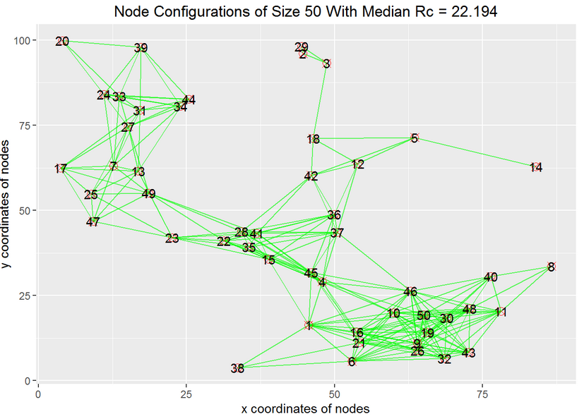
- We also want to study the distribution of $R_c$ for different configurations of the nodes.

---

# Simulation Study for Ad Hoc Network

1. We will randomly generate nodes for an ad hoc network according to some pre-specified node density (generally determined by the geographical information).


.pull-left[

<p align="center">
<img src="./figures/contour_3d.jpeg" width="400"/>
</p>

]

.pull-right[

<p align="center">
<img src="./figures/contour_2d.jpg" width="400"/>
</p>

]

---

# Simulation Study for Ad Hoc Network

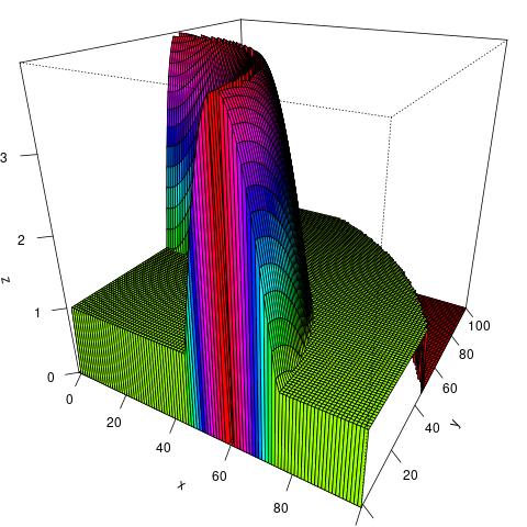
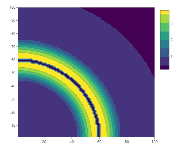
1. We will randomly generate $n$ nodes for an ad hoc network according to some pre-specified node density (generally determined by the geographical information). Specifically, we will use the acceptance-rejection algorithm.

- Generate points uniformly in a three-dimensional rectangle.

- If the points fall in the three-dimensional region beneath the density, then we keep them.

- Use the $(x,y)$ coordinates of these accepted points as our sample.

---

# Simulation Study for Ad Hoc Network

1. We will randomly generate $n$ nodes for an ad hoc network according to some pre-specified node density (generally determined by the geographical information).

2. Find the smallest $R_c$ such that the nodes are connected through paths in the network.

3. Repeat several times for each $n$.

4. Study the distribution of $R_c$.

[Project Description](https://raw.githubusercontent.com/zhangyk8/zhangyk8.github.io/master/_teaching/file_stat302/Lectures/Final_Project.pdf)

---
# Summary

- Running simulations is an integral part of being a modern statistician.

- R provides us with several utility functions for simulations from a wide variety of distributions.

- To make our simulation results reproducible, we must set the seed via `set.seed()`.

- Monte Carlo methods provide us with feasible ways to compute integrals or sample observations from a given density function.

- The bootstrap principle presents an almost distribution-free way to quantify the uncertainties of our statistical estimators. 

Submit Lab 6 on Canvas by the end of Thursday (February 29) and the final project by the end of March 13!!