---
title: "STAT 302 Statistical Computing"
subtitle: "Lecture 9: Statistical Prediction"
author: "Yikun Zhang (_Winter 2024_)"
date: ""
output:
  xaringan::moon_reader:
    css: ["uw.css", "fonts.css"]
    lib_dir: libs
    nature:
      highlightStyle: tomorrow-night-bright
      highlightLines: true
      countIncrementalSlides: false
      titleSlideClass: ["center","top"]
---

```{r setup, include=FALSE, purl=FALSE}
options(htmltools.dir.version = FALSE)
knitr::opts_chunk$set(comment = "##")
library(kableExtra)
```

# Outline

1. Statistical Regression Model

2. Statistical Prediction and Cross-Validation

3. Bias-Variance Trade-off

3. Topics that Were Not Covered

<p><font size="4">* Acknowledgement: Parts of the slides are modified from the course materials by Prof. Ryan Tibshirani and Bryan Martin. </font></p>

---
class: inverse

# Part 1: Statistical Regression Model

---

# Statistical Regression Model

Assume that we have some generic variables $X_1,\ldots,X_p, Y$, where
- $X_1,...,X_P$ are $p$ **independent variables** or **explanatory variables** or **covariates** or **predictors** or **features**.

- $Y$ is the **dependent variable** or **response** or **outcome**.

--

We want to know the relationship between the covariates and the response. 

- Suppose we posit that $Y|X_1,...,X_p \sim P$, where $P$ is some unknown distribution.

- This is called **regression model** for $Y$ given $X_1,...,X_p$.

--

The goal of regression is to estimate the unknown distribution $P$ from the observed data under some (model) assumptions.

---

# Importance of Statistical Regression Models

The regression model provides us with a statistical approach to conduct

- **Inference:** assess the model validity, analyze the relationship between the covariates, study the covariate importance, etc.
  - What is the relationship between sleeping time and GPA?
  
  - Is parents' education or parents' income more important for explaining their children's income?
  
--
  
- **Prediction:** predict new/future outcomes $Y$'s from new/future covariates $X_1,...,X_p$'s.
  * Can we predict test scores based on hours spent studying?
  
---

# Linear Regression Model

The linear model is arguably the _most widely used_ statistical model, which has a place in nearly every application domain of statistics.

Given response $Y$ and predictors $X_1,...,X_p$ in a **linear regression model**, we posit that
$$Y = \beta_0+\beta_1 X_1 + \cdots +\beta_p X_p + \epsilon \quad \text{ with } \quad \epsilon \sim N(0,\sigma^2).$$

--

The goal is to estimate the (model) parameters $\beta_0,\beta_1,...,\beta_p$, which are also called **coefficients**.

- **Inference:** To assess whether the linear model is true, which covariates are important.

- **Prediction:** To simply predict future $Y$'s from future $X_1,...,X_p$'s.

---

# $\large \epsilon$: Error term

$\epsilon$ represents the **error term** of our model. Why do we need to incorporate this error term?

--

We model $Y$ as a linear function of $X_1,...,X_p$, but in the real world, the linear relationship won't always be perfect, because

* Measurement error in the $X$'s.

* Measurement error in the $Y$'s.

* Unobserved/latent variables beyond the current covariates $X_1,...,X_p$.

* Deviations in the true model from linearity.

* True randomness.

Note: In the linear regression, we assume that this error term is normally distributed with mean $0$ and variance $\sigma^2$.

---

# $\beta_0$: Intercept

$\beta_0$ is the **intercept term** of our model. 

- Notice that 

$$\large \mathbb{E}[Y|X_1 = X_2 = \cdots = X_p = 0] = \beta_0.$$

- Thus, $\beta_0$ is the expected value of our response if all the covariates are equal to $0$!

- This is also known as the $y$-intercept of our model.

---

# $\beta_j$: $j^{th}$ Coefficient

$X_j$ represents the $j^{th}$ independent variable/covariate in our model. 

- Notice that 
$$\large \mathbb{E}[Y|X_1,\ldots, X_p] = \beta_0 + \beta_1 X_1 + \cdots + \beta_p X_p.$$

What happens to this expectation if we increase $X_j$ by 1 unit, holding everything else constant?

--

- The conditional expectation of $Y$ increases by $\beta_j$!

- **Interpretation of $\beta_j$:** the expected difference in the response between two observations differing by one unit in $X_j$, with all other covariates identical.

---

# Linear Regression

$$\large Y = \beta_0+\beta_1 X_1 + \cdots \beta_p X_p + \epsilon \quad \text{ with } \quad \epsilon \sim N(0,\sigma^2).$$


* $Y$: dependent variable, outcome, response.

* $X_j$: independent variable, covariate, predictor, feature.

* $\beta_0$: Intercept.

* $\beta_j$: coefficient, the expected difference in the response between two observations differing by one unit in $X_j$, with all other covariates identical.

* $\epsilon$: error, noise, normally distributed with mean $0$ and variance $\sigma^2$.

--

Given the training data $\{(Y_i,X_{i,1},...,X_{i,p})\}_{i=1}^n$, we fit $\hat{\beta}_0,...,\hat{\beta}_p$ by minimizing the mean square error
$$\sum_{i=1}^n\left(Y_i - \beta_0-\beta_1X_{i,1}-\cdots -\beta_pX_{i,p}\right)^2.$$

---


# Matrix Notation

We can fully write out a linear regression model

\\[
\begin{equation}
\begin{bmatrix} Y_1 \\ Y_2\\ \vdots \\ Y_n \end{bmatrix} = 
\begin{bmatrix} 1 & X_{1,1} & \cdots & X_{1,p}\\
1 & X_{2,1} & \cdots & X_{2, p}\\
\vdots & \vdots & \ddots & \vdots \\
1 & X_{n,1} & \cdots & X_{n, p}\end{bmatrix}
\begin{bmatrix} \beta_0 \\ \beta_1 \\ \vdots \\ \beta_n \end{bmatrix} +
\begin{bmatrix} \epsilon_1 \\ \epsilon_2 \\ \vdots \\ \epsilon_{n} \end{bmatrix}
\end{equation}
\\]

This can also be expressed in matrix form:
\\[
\begin{align}
\mathbf{Y} &= \mathbf{X}\beta + \epsilon,\quad \epsilon\sim N(0,1)
\end{align}
\\]
* $\mathbf{Y} \in \mathbb{R}^{n \times 1}$: an $n$-dimensional vector of the response.
* $\mathbf{X} \in \mathbb{R}^{n \times (p+1)}$: a $(p+1)\times n$ matrix of the predictors (including intercept).
* $\mathbf{\beta} \in \mathbb{R}^{(p+1)\times 1}$: a $(p+1)$-dimensional vector of regression parameters.
* $\mathbf{\epsilon} \in \mathbb{R}^{n \times 1}$: an $n$-dimensional vector of the error term.

---

# Linear Regression in R

We fit a linear regression model in R using the function `lm()`.

```{r}
data(mtcars)
my_lm = lm(mpg ~ hp + wt, data = mtcars)
```

--

- The first argument is a **formula**, which is a type of R object. The formula typically takes the form: `Y ~ X1 + X2 + ... + Xp`.

  - The dependent variable `Y` goes on the left-hand side of the tilde `~`, which marks the formula. 

  - The independent variables are added on the right-hand side.
  
- Using this formula will give us a model in the form of
\\[
\begin{eqnarray}
&Y &= \beta_0 + \beta_1 X_1 + \cdots + \beta_p X_p + \epsilon, \quad \epsilon &\sim N(0,\sigma^2).
\end{eqnarray}
\\]


---

# Linear Regression in R (Example)

```{r}
data(mtcars)
my_lm = lm(mpg ~ hp + wt, data = mtcars)
class(my_lm)
my_lm
```

We can see from `names()` that `lm` objects contain a lot more than they print out by default.
```{r}
names(my_lm)
```


---

# Linear Regression in R (Example)

The function `summary()` gives us a summary of our `lm` object in R.

* The quantiles of the residuals: hopefully, they match a normal distribution!

* Coefficients, their standard errors, and their individual significance levels.

* (Adjusted) R-squared value: how much of the overall variability in the response is explained by the model?

* F-statistic: hypothesis test for the significance of the overall model.

---

# Linear Regression in R (Example)

```{r}
summary(my_lm)
```


---

# Model Diagnostics on Linear Regression

Calling `plot()` on the `lm` object will return several diagnostic plots.

- Recall that we want the error term to look normally distributed with mean zero.

We won't go into the details for this class, but here are some tips:

* **Residuals vs Fitted:** these are the errors (residuals) plotted over the predicted outcome (fitted). Errors should be random, so we want to see randomly scattered points with no discernible patterns, and the trend line should be approximately horizontal.

* **Normal Q-Q plot:** These are the quantiles of the errors against the quantiles of a normal distribution. In theory, the errors should be normally distributed, so those points should be mostly along the 45-degree $y=x$ line.

---

# Model Diagnostics on Linear Regression

Calling `plot()` on the `lm` object will return several diagnostic plots.

* **Scale-location:** This looks at the magnitude of standardized residuals over the predicted outcome. Similar interpretation as **residuals vs fitted**, which make it slightly easier to identify undesirable patterns.

* **Residuals vs leverage:** This can help identify highly influential points, such as outliers. If points are outside dotted red lines, then removing them would noticeably alter the linear regression results. *Never simply remove outliers!* 

  - If we work on real data, it is valid and removing it will bias your results. Removing clearly mis-entered data is fine. It is much more important to understand why outliers are there than to remove them.

---

# Model Diagnostics on Linear Regression

```{r, eval = FALSE}
plot(my_lm)
```

.center[
```{r, echo = FALSE}
plot(my_lm, which = 1)
```
]

---

# Model Diagnostics on Linear Regression

```{r, eval = FALSE}
plot(my_lm)
```

.center[
```{r, echo = FALSE}
plot(my_lm, which = 2)
```
]

---

# Model Diagnostics on Linear Regression

```{r, eval = FALSE}
plot(my_lm)
```

.center[
```{r, echo = FALSE}
plot(my_lm, which = 3)
```
]
---

# Model Diagnostics on Linear Regression

```{r, eval = FALSE}
plot(my_lm)
```

.center[
```{r, echo = FALSE}
plot(my_lm, which = 5)
```
]

---

# Linear Regression Results

We use the function `coef()` to extract estimated coefficients as a vector.

```{r}
coef(my_lm)
```

--

We use the function `fitted()` to extract the fitted/estimated values for the response. This is also known as **in-sample prediction**. 

```{r}
fitted(my_lm)
```


---

# Linear Regression Results

It is also useful to compare how our fitted values with the estimated values in order to assess the model fitting.

```{r, include=FALSE}
library(ggplot2)
```


```{r, fig.height = 3.5, eval = FALSE}
mod_fits = fitted(my_lm)
my_df = data.frame(actual = mtcars$mpg, fitted = mod_fits)
ggplot(my_df, aes(x = fitted, y = actual)) +
  geom_point() +
  geom_abline(slope = 1, intercept = 0, col = "red", lty = 2) + 
  theme_bw(base_size = 15) +
  labs(x = "Fitted values", y = "Actual values", title = "Actual vs. Fitted") +
  theme(plot.title = element_text(hjust = 0.5))
```


.center[
```{r, fig.height = 3.5, echo = FALSE}
mod_fits <- fitted(my_lm)
my_df <- data.frame(actual = mtcars$mpg, fitted = mod_fits)
ggplot(my_df, aes(x = fitted, y = actual)) +
  geom_point() +
  geom_abline(slope = 1, intercept = 0, col = "red", lty = 2) + 
  theme_bw(base_size = 15) +
  labs(x = "Fitted values", y = "Actual values", title = "Actual vs. Fitted") +
  theme(plot.title = element_text(hjust = 0.5))
```
]

---

# Out-of Sample Prediction By Linear Regression

We use the function `predict()` to predict the responses given new covariates. This is also known as the **out-of-sample prediction**.

- For example, suppose that we observe two new cars with gross horse powers of `100` and `150`, respectively, and weights of `3000` lbs and `3500` lbs, respectively.

```{r}
# Note: wt is in 1000s of lbs!
new_obs = data.frame(hp = c(100, 150), wt = c(3, 3.5))
predict(my_lm, new_obs)
```

---
class: inverse

# Part 2: Statistical Prediction and Cross-Validation

---

# Good Interpretation or Good Prediction?

Often, we start our statistical modeling by fitting the linear models, because they are simple and interpretable.

--

- In many cases, the true data generating process is nonlinear, and the errors are by no means close to Gaussian or homoskedastic.

--

- There are many other prediction models that have been developed:

  - Logistic regression, Poisson regression, and other generalized linear models.
  
  - Generalized additive models.
  
  - Nonparametric models, Bayesian models, and complicated machine learning models.
  
The key for good prediction is to have a standard criterion to evaluate the **prediction accuracy** of our chosen model.

---

# Training and Test Errors

**Training data:** the data that we use to train/fit our model.

**Test data:** the holdout/future data that we use to evaluate/test the performance of our model.

--

Linear regression example:

- Suppose we use the training data $\{(Y_i,X_{i,1},...,X_{i,p})\}_{i=1}^n$ to estimate the regression coefficients $\hat{\beta}_0,...,\hat{\beta}_p$.

- Given new covariates $X_1^*,...,X_p^*$, we are asked to predict the associated $Y^*$ on this test point/data. 

- By the estimated linear model, we predict
$$\hat{Y}^*=\hat{\beta}_0+\hat{\beta}_1X_1^* + \cdots + \hat{\beta}_p X_p^*.$$

---

# Training and Test Errors

We define the **test error**, also called prediction error, under the square loss function $L(Y,Y')=(Y-Y')^2$ by 
$$\mathbb{E}\left[L\left(Y^*, \hat{Y}^*\right) \right] = \mathbb{E}\left[\left(Y^* - \hat{Y}^*\right)^2 \right],$$
where the expectation is taken over every random quantity: the training data $\{(Y_i,X_{i,1},...,X_{i,p})\}_{i=1}^n$ and test data $(Y^*, X_1^*,...,X_p^*)$.

--

We define the **training error** under the square loss function $L(Y,Y')=(Y-Y')^2$ by 
$$\frac{1}{n} \sum_{i=1}^n L\left(Y_i,\hat{Y}_i\right) = \frac{1}{n}\sum_{i=1}^n \left(Y_i - \hat{Y}_i\right)^2.$$

Note: We explain the training and test errors for a linear model, but the same definitions hold in general.

---

# Training and Test Errors

Test error: $\mathbb{E}\left[L\left(Y^*, \hat{Y}^*\right) \right] = \mathbb{E}\left[\left(Y^* - \hat{Y}^*\right)^2 \right]$.

Training error: $\frac{1}{n} \sum\limits_{i=1}^n L\left(Y_i,\hat{Y}_i\right) = \frac{1}{n}\sum\limits_{i=1}^n \left(Y_i - \hat{Y}_i\right)^2$.

- The definition of the _test error_ relies on the out-of-sample prediction $\hat{Y}^*$ from the model.

- The _training error_, on the contrary, is defined through the in-sample predictions
$$\hat{Y}_i = \hat{\beta}_0+\hat{\beta}_1X_{i,1} + \cdots + \hat{\beta}_p X_{i,p} \quad \text{ for } \quad i=1,...,n.$$

---

# Estimating Test Error

The test error, $\mathbb{E}\left[L\left(Y^*, \hat{Y}^*\right) \right] = \mathbb{E}\left[\left(Y^* - \hat{Y}^*\right)^2 \right]$, quantifies the expected squared difference between a new prediction and the truth.

  - **Predictive Assessment:** It provides us with a valid way to assess the magnitude of errors of our model in making future predictions!
  
  - **Model Selection:** It helps us choose among different models/methods that could minimize the test error.
  
--
  
Question: How do we estimate the test error?

- Note that it is generally impossible to compute that expectation.

---

# Estimating Test Error

Question: How do we estimate the test error?

- Note that it is generally impossible to compute that expectation.

- Can we estimate it by the training error? 

--

- Generally, the training error is **too optimistic** for estimating the test error, because the parameters $\hat{\beta}_0,...,\hat{\beta}_p$ were estimated to make $\hat{Y}_i$ close to $Y_i$ for $i=1,...,n$ in the first place!

- In most cases, the more **complex/adaptive** the model, the more optimistic its training error is as an estimate of the test error.

---

# Training Error vs Test Error (Example)

```{r, fig.align = "center", fig.height = 6, fig.width=8}
# generate data
set.seed(302)
n = 30
x = sort(runif(n, -3, 3))
y = 2*x + 2*rnorm(n)
x_test = sort(runif(n, -3, 3))
y_test = 2*x_test + 2*rnorm(n)
df_train = data.frame("x" = x, "y" = y)
df_test = data.frame("x" = x_test, "y" = y_test)

par(mfrow=c(1,2))
xlim = range(c(x, x_test)); ylim = range(c(y, y_test))
plot(x, y, xlim=xlim, ylim=ylim, main="Training data")
plot(x_test, y_test, xlim=xlim, ylim=ylim, main="Test data")
```


---

# Training Error vs Test Error (Degree 1 Model)

```{r, eval=FALSE}
lm_fit = lm(y ~ x, data = df_train)
yhat_train1 = predict(lm_fit)
train_err1 = mean((df_train$y - yhat_train1)^2)
# Calculate test error
yhat_test1 = predict(lm_fit, data.frame(x = df_test$x))
test_err1 = mean((df_test$y - yhat_test1)^2)

par(mfrow=c(1,2))
plot(x, y, xlim=xlim, ylim=ylim, main=paste("Training data (Training error:", round(train_err1, 3), ")"))
lines(x, yhat_train1, col=2, lwd=3)

plot(x_test, y_test, xlim=xlim, ylim=ylim, main=paste("Test data (Test error:", round(test_err1, 3), ")"))
lines(x_test, yhat_test1, col=3, lwd=3)
```

---

# Training Error vs Test Error (Degree 1 Model)

```{r, fig.align = "center", fig.height = 7, fig.width=9, echo=FALSE}
lm_fit = lm(y ~ x, data = df_train)
yhat_train1 = predict(lm_fit)
train_err1 = mean((df_train$y - yhat_train1)^2)
# Calculate test error
yhat_test1 = predict(lm_fit, data.frame(x = df_test$x))
test_err1 = mean((df_test$y - yhat_test1)^2)

par(mfrow=c(1,2))
plot(x, y, xlim=xlim, ylim=ylim, main=paste("Training data (Training error:", round(train_err1, 3), ")"))
lines(x, yhat_train1, col=2, lwd=3)

plot(x_test, y_test, xlim=xlim, ylim=ylim, main=paste("Test data (Test error:", round(test_err1, 3), ")"))
lines(x_test, yhat_test1, col=3, lwd=3)
```

---

# Training Error vs Test Error (Degree 5 Model)

```{r, eval=FALSE}
# Fit 5 degree polynomial and calculate training error
lm_fit_5 = lm(y ~ poly(x, 5), data = df_train)
yhat_train5 = predict(lm_fit_5)
train_err5 = mean((df_train$y - yhat_train5)^2)

# Calculate testing error
yhat_test5 = predict(lm_fit_5, data.frame(x = df_test$x))
test_err5 = mean((df_test$y - yhat_test5)^2)

# Create smooth line for plotting
x_fit = seq(-3, 3, length = 100)
y_fit = predict(lm_fit_5, newdata = data.frame(x = x_fit))

par(mfrow=c(1,2))
plot(x, y, xlim=xlim, ylim=ylim, main=paste("Training data (Training error:", round(train_err5, 3), ")"))
lines(x_fit, y_fit, col=2, lwd=3)

plot(x_test, y_test, xlim=xlim, ylim=ylim, main=paste("Test data (Test error:", round(test_err5, 3), ")"))
lines(x_fit, y_fit, col=3, lwd=3)
```

---

# Training Error vs Test Error (Degree 5 Model)

```{r, fig.align = "center", fig.height = 7, fig.width=9, echo=FALSE}
# Fit 5 degree polynomial and calculate training error
lm_fit_5 = lm(y ~ poly(x, 5), data = df_train)
yhat_train5 = predict(lm_fit_5)
train_err5 = mean((df_train$y - yhat_train5)^2)

# Calculate testing error
yhat_test5 = predict(lm_fit_5, data.frame(x = df_test$x))
test_err5 = mean((df_test$y - yhat_test5)^2)

# Create smooth line for plotting
x_fit = seq(-3, 3, length = 100)
y_fit = predict(lm_fit_5, newdata = data.frame(x = x_fit))

par(mfrow=c(1,2))
plot(x, y, xlim=xlim, ylim=ylim, main=paste("Training data (Training error:", round(train_err5, 3), ")"))
lines(x_fit, y_fit, col=2, lwd=3)

plot(x_test, y_test, xlim=xlim, ylim=ylim, main=paste("Test data (Test error:", round(test_err5, 3), ")"))
lines(x_fit, y_fit, col=3, lwd=3)
```

---

# Training Error vs Test Error (Degree 10 Model)

```{r, eval=FALSE}
# Fit 10 degree polynomial and calculate training error
lm_fit_10 = lm(y ~ poly(x, 10), data = df_train)
yhat_train10 = predict(lm_fit_10)
train_err10 = mean((df_train$y - yhat_train10)^2)

# Calculate testing error
yhat_test10 = predict(lm_fit_10, data.frame(x = df_test$x))
test_err10 = mean((df_test$y - yhat_test10)^2)

# Create smooth line for plotting
x_fit = seq(-3, 3, length = 100)
y_fit = predict(lm_fit_10, newdata = data.frame(x = x_fit))

par(mfrow=c(1,2))
plot(x, y, xlim=xlim, ylim=ylim, main=paste("Training data (Training error:", round(train_err10, 3), ")"))
lines(x_fit, y_fit, col=2, lwd=3)

plot(x_test, y_test, xlim=xlim, ylim=ylim, main=paste("Test data (Test error:", round(test_err10, 3), ")"))
lines(x_fit, y_fit, col=3, lwd=3)
```

---

# Training Error vs Test Error (Degree 10 Model)

```{r, fig.align = "center", fig.height = 7, fig.width=9, echo=FALSE}
# Fit 10 degree polynomial and calculate training error
lm_fit_10 = lm(y ~ poly(x, 10), data = df_train)
yhat_train10 = predict(lm_fit_10)
train_err10 = mean((df_train$y - yhat_train10)^2)

# Calculate testing error
yhat_test10 = predict(lm_fit_10, data.frame(x = df_test$x))
test_err10 = mean((df_test$y - yhat_test10)^2)

# Create smooth line for plotting
x_fit = seq(-3, 3, length = 100)
y_fit = predict(lm_fit_10, newdata = data.frame(x = x_fit))

par(mfrow=c(1,2))
plot(x, y, xlim=xlim, ylim=ylim, main=paste("Training data (Training error:", round(train_err10, 3), ")"))
lines(x_fit, y_fit, col=2, lwd=3)

plot(x_test, y_test, xlim=xlim, ylim=ylim, main=paste("Test data (Test error:", round(test_err10, 3), ")"))
lines(x_fit, y_fit, col=3, lwd=3)
```

---

# Training Error vs Test Error (Degree 15 Model)

```{r, eval=FALSE}
# Fit 15 degree polynomial and calculate training error
lm_fit_15 = lm(y ~ poly(x, 15), data = df_train)
yhat_train15 = predict(lm_fit_15)
train_err15 = mean((df_train$y - yhat_train15)^2)

# Calculate testing error
yhat_test15 = predict(lm_fit_15, data.frame(x = df_test$x))
test_err15 = mean((df_test$y - yhat_test15)^2)

# Create smooth line for plotting
x_fit = seq(-3, 3, length = 100)
y_fit = predict(lm_fit_15, newdata = data.frame(x = x_fit))

par(mfrow=c(1,2))
plot(x, y, xlim=xlim, ylim=ylim, main=paste("Training data (Training error:", round(train_err15, 3), ")"))
lines(x_fit, y_fit, col=2, lwd=3)

plot(x_test, y_test, xlim=xlim, ylim=ylim, main=paste("Test data (Test error:", round(test_err15, 3), ")"))
lines(x_fit, y_fit, col=3, lwd=3)
```

---

# Training Error vs Test Error (Degree 15 Model)

```{r, fig.align = "center", fig.height = 7, fig.width=9, echo=FALSE}
# Fit 15 degree polynomial and calculate training error
lm_fit_15 = lm(y ~ poly(x, 15), data = df_train)
yhat_train15 = predict(lm_fit_15)
train_err15 = mean((df_train$y - yhat_train15)^2)

# Calculate testing error
yhat_test15 = predict(lm_fit_15, data.frame(x = df_test$x))
test_err15 = mean((df_test$y - yhat_test15)^2)

# Create smooth line for plotting
x_fit = seq(-3, 3, length = 100)
y_fit = predict(lm_fit_15, newdata = data.frame(x = x_fit))

par(mfrow=c(1,2))
plot(x, y, xlim=xlim, ylim=ylim, main=paste("Training data (Training error:", round(train_err15, 3), ")"))
lines(x_fit, y_fit, col=2, lwd=3)

plot(x_test, y_test, xlim=xlim, ylim=ylim, main=paste("Test data (Test error:", round(test_err15, 3), ")"))
lines(x_fit, y_fit, col=3, lwd=3)
```

---

# Sample-Splitting

How can we estimate the test error given a single data set? (Assuming that we cannot simulate more data for testing.)

- We know that the training error is too optimistic.

--

- A tried-and-true technique with an old history in statistics called **sample-splitting** works well in practice.

  1. Split the data set into two parts (e.g., 80% vs 20% or 50% vs 50%).
  
  2. Train the model/method on the first part.
  
  3. Make predictions and evaluate the test errors on the second part.
  
---

# Sample-Splitting (Example)

```{r}
dat = read.table("https://github.com/zhangyk8/zhangyk8.github.io/raw/master/_teaching/file_stat302/Data/xy.dat")
head(dat)
n = nrow(dat)
# Randomly split the data into two parts
set.seed(123)
inds = sample(c(rep(1, length = round(0.8*n)), rep(2, length = n - round(0.8*n))))
train_set = dat[inds == 1,]
test_set = dat[inds == 2,]
```

---

# Sample-Splitting (Example)

```{r}
# Train on the first half
lm.1 = lm(y ~ x, data=train_set)
lm.10 = lm(y ~ poly(x,10), data=train_set)

# Predict on the second half and evaluate test error
pred.1 = predict(lm.1, data.frame(x=test_set$x))
pred.10 = predict(lm.10, data.frame(x=test_set$x))

test.err.1 = mean((test_set$y - pred.1)^2)
test.err.10 = mean((test_set$y - pred.10)^2)
```

---

# Sample-Splitting (Example)

```{r, fig.align = "center", fig.height=6.5, fig.width=9}
# Plot the results
par(mfrow=c(1,2))
xx = seq(min(dat$x), max(dat$x), length=100)

plot(dat$x, dat$y, pch=c(21,19)[inds], main=paste("Degree 1 (Test error:", round(test.err.1, 3), ")"), xlab = "X", ylab = "Y")
lines(xx, predict(lm.1, data.frame(x=xx)), col=2, lwd=2)
legend("topleft", legend=c("Training","Test"), pch=c(21,19))

plot(dat$x, dat$y, pch=c(21,19)[inds], main=paste("Degree 10 (Test error:", round(test.err.10, 3), ")"), xlab = "X", ylab = "Y")
lines(xx, predict(lm.10, data.frame(x=xx)), col=3, lwd=2)
legend("topleft", legend=c("Training","Test"), pch=c(21,19))
```

---

# Cross-validation

Sample-splitting is simple and effective. However, it estimates the test error when the model/method is trained on **less data** (say, 80% of the full data set).

--

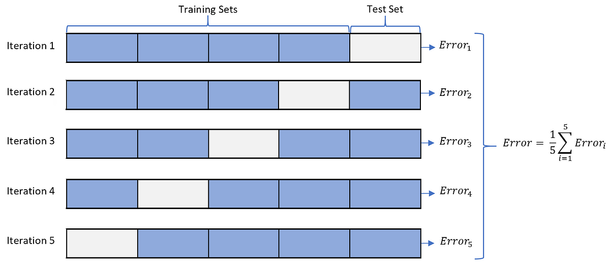
One improvement over sample splitting is **k-fold cross-validation**.

1. Split data into $k$ parts or folds.

2. Use all but one fold to train the model/method.

3. Use the hold-out fold to make prediction and evaluate a test error.

4. Rotate around the roles of folds, which has $k$ rounds in total.

5. Compute the average test errors across all folds in the end.

---

# Cross-Validation

A common choice is $k=5$ or $k=10$ (sometimes $k=n$, which is known as the **leave-one-out** cross-validation (LOOCV)!)

<p align="center">
<img src="./figures/cv-result.png" width="800"/>

Note: The LOOCV has its own drawback, because it fits $n$ models that are trained on almost identical training data and the outputs of these models are highly (positively) correlated. When all other things being equal, the LOOCV estimated test error has a higher variance than the test error from $k$-fold cross-validation when $k\ll n$. 

---

# Cross-Validation (Example)

```{r}
# Randomly split data in 5 parts
k = 5
set.seed(123)
inds = sample(rep(1:k, length=n))
table(inds)

# Now run cross-validation: easiest with for loop
pred.mat = matrix(0, n, 2) # Empty matrix to store predictions
for (i in 1:k) {
  cat(paste("Fold",i,"... "))
  
  train_set = dat[inds!=i,] # Training data
  test_set = dat[inds==i,] # Test data
  # Train our models
  lm.1.minus.i = lm(y ~ x, data=train_set)
  lm.10.minus.i = lm(y ~ poly(x,10), data=train_set)
  # Record predictions
  pred.mat[inds==i,1] = predict(lm.1.minus.i, data.frame(x=test_set$x))
  pred.mat[inds==i,2] = predict(lm.10.minus.i, data.frame(x=test_set$x))
}
```

---

# Cross-Validation (Example)

```{r, fig.align = "center", fig.height=6.5, fig.width=9}
# Compute cross-validation error, one for each model
cv.errs = colMeans((pred.mat - dat$y)^2)

# Plot the results
par(mfrow=c(1,2))
xx = seq(min(dat$x), max(dat$x), length=100)

plot(dat$x, dat$y, pch=20, col=inds+1, main=paste("Degree 1 (Test error:", round(cv.errs[1], 3), ")"), xlab = "X", ylab = "Y")
lines(xx, predict(lm.1, data.frame(x=xx)), lwd=2, lty=2) 
legend("topleft", legend=paste("Fold",1:k), pch=20, col=2:(k+1))

plot(dat$x, dat$y, pch=20, col=inds+1, main=paste("Degree 10 (Test error:", round(cv.errs[2], 3), ")"), xlab = "X", ylab = "Y")
lines(xx, predict(lm.10, data.frame(x=xx)), lwd=2, lty=2) 
legend("topleft", legend=paste("Fold",1:k), pch=20, col=2:(k+1))
```

---
class: inverse

# Part 3: Bias-Variance Trade-off

---

# Bias-Variance Trade-off

The test error can be decomposed as a function of the bias and variance of our estimates. For instance, under the square loss $L(Y,Y')=(Y-Y')^2$, we have that 
$$\mathbb{E}\left[\left(Y^* - \hat{Y}^*\right)^2 \right] = \underbrace{\mathbb{E}\left[\left(Y^* - \mathbb{E}\hat{Y}^*\right)^2 \right]}_{\mathbb{E}\left(\text{Bias}^2\right)} + \underbrace{\mathbb{E}\left[\left(\hat{Y}^* - \mathbb{E}\hat{Y}^*\right)^2 \right]}_{\text{Variance}}$$

* **Bias:** the expected difference between our estimates and the truth values.

* **Variance:** the variability of our estimates.

---

# Bias-Variance Trade-off

* **Bias:** the expected difference between our estimates and the truth values.

* **Variance:** the variability of our estimates.

<p align="center">
<img src="./figures/bvtradeoff.png" width="500"/>
</p>
<p align="center">
<font size="4">Image credit: <a href="https://www.statlearning.com/">An Introduction to Statistical Learning</a> by Gareth James, Daniela Witten, Trevor Hastie, Robert Tibshirani.</font>
</p>

---

# Bias-Variance Trade-off

Generally, how well the model fits the training data can reflect its bias and variance.

- A simple model would **underfit** the training data, which leads to _high bias_ and _low variance_.

- A complex model would **overfit** the training data, which leads to _low bias_ and _high variance_.

<p align="center">
<img src="./figures/overfit2.webp" width="750"/>
</p>

---

# Bias-Variance Trade-off

Generally, how well the model fits the training data can reflect its bias and variance.

- A simple model would **underfit** the training data, which leads to _high bias_ and _low variance_.

- A complex model would **overfit** the training data, which leads to _low bias_ and _high variance_.

<p align="center">
<img src="./figures/overfitting.png" width="750"/>
</p>

---

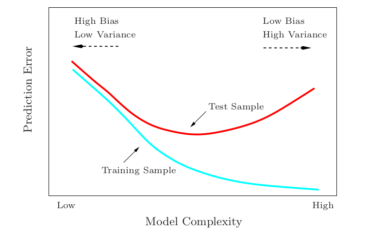
# Bias-Variance Trade-off

Bias-variance trade-off is also considered as a central tenet in machine learning.

<p align="center">
<img src="./figures/bias_var.png" width="800"/>
</p>

---

# Machine Learning Practice

The standard machine learning practice is to find/tune the model to be as close to the "sweet spot" as possible.

<p align="center">
<img src="./figures/bias_var_risk.png" width="650"/>
</p>

Note: Test risk = test error; training risk = training error; capacity of the space $\mathcal{H}$ $\approx$ model complexity.

---

# Machine Learning Practice

There are several ways to pursue the "sweet-spot" model from a given class of models.

- Use the cross-validation to select the optimal parameters for the model.

- Add some regularization to the complex model to prevent overfitting.

- Pick a relatively simple model from the candidate class ([Occam's razor](https://en.wikipedia.org/wiki/Occam%27s_razor)).

---

# Machine Learning Practice

To become a machine learning or artificial intelligence (AI) engineer, we only need to

1. Understand the bias-variance trade-off principle.

2. Know how to do computer programming.

3. Avoid overfitting with the preceding standard techniques.

--

<p align="center">
<img src="./figures/Kid_Prom.jpeg" width="300"/>
</p>
<p align="center">
<font size="4"> The picture is an AI textbook designed for children at the kindergarten level in China. There are some news saying that several
kindergartens are teaching computer programming to their 3-5 years-old kids.</font>
</p>

---

# Contradictory Evidence from Deep Learning

<p align="center">
<img src="./figures/NN_eg.png" width="700"/>
</p>

<p align="center">
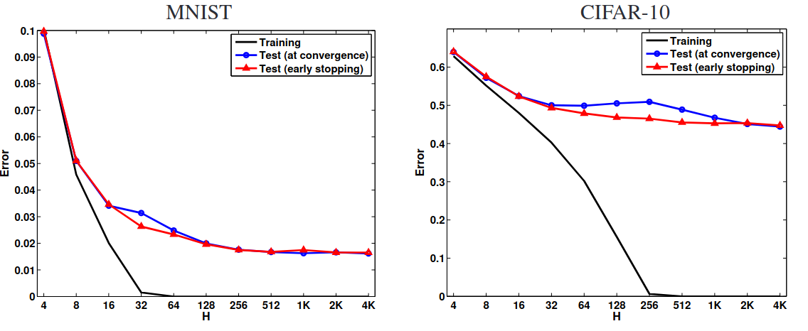
<font size="4"> The training and test errors of two-layer neural networks with different numbers of hidden units H that were trained on MNIST and CIFAR-10 datasets (<a href="https://arxiv.org/abs/1412.6614">Neyshabur et al., 2014</a>).</font>
</p>

---

# Modern View of the Bias-Variance Trade-off: "Double-Descent" Curve

<p align="center">
<img src="./figures/double_descent.jpg" width="800"/>
</p>

<p align="center">
<font size="4"> Image source and reference paper: <a href="https://www.pnas.org/doi/10.1073/pnas.1903070116">Belkin et al. (2019)</a>.</font>
</p>

---
class: inverse

# Part 4: Topics that Were Not Covered

---

# Other Interesting Topics

Here are some potential topics that other Statistical Computing courses may cover:

- Text Mining and Regular Expression: 
  - [Reference slides for regular expressions](https://bryandmartin.github.io/STAT302/docs/LectureSlides/lectureslides4_stringsfactors/lectureslides_stringsfactors.html#1); 
  - [Reference book for text mining in R](https://www.tidytextmining.com/).

- Rational Database in R: [Reference slides](https://www.stat.cmu.edu/~ryantibs/statcomp/lectures/databases_slides.html#1).

- JSON, XML, and Web Scraping in R: [Reference webpage](https://steviep42.github.io/webscraping/book/xml.html).

- R Shiny: 
  - [Reference webpage](https://mastering-shiny.org/basic-app.html);
  - [STAT 451 Visualizing Data](https://stat.uw.edu/academics/course-catalog/stat-451).
  
- Resampling Method and Bootstrap: [STAT 403 Introduction to Resampling Inference](https://stat.uw.edu/academics/course-catalog/stat-403).

---

# Other Interesting Topics

- Version Control and Statistical Software Development (R Package):
  - [Reference webpage for version control and Git](https://happygitwithr.com/).
  - [STAT 498 Agile Data Science](https://uwnetid-my.sharepoint.com/:b:/r/personal/abelrod_uw_edu/Documents/Special%20topics/syllabus_STAT498_Wadswoth_Winter2024.pdf?csf=1&web=1&e=c45oid) (Only open for Winter 2024).
  - [Reference slides for Creating R Packages](https://bryandmartin.github.io/STAT302/docs/LectureSlides/lectureslides9_package/lectureslides_package.html#1).
  - [Tutorial webpage for Creating R Packages](https://kbroman.org/pkg_primer/).

- Optimization: 
  - [Reference webpage](https://bookdown.org/rdpeng/advstatcomp/general-optimization.html).
  - [MATH 407 Linear Optimization](https://math.washington.edu/courses/2024/winter/math/407/a), [MATH 408 Nonlinear Optimization](https://math.washington.edu/courses/2024/winter/math/408/a).
  - [Reference Book: Convex Optimization](https://web.stanford.edu/~boyd/cvxbook/bv_cvxbook.pdf), [Free online course I](https://see.stanford.edu/Course/EE364A), [Free online course II](https://www.stat.cmu.edu/~ryantibs/convexopt/).

- [STAT 133 Concepts in Computing With Data at UC Berkeley](https://github.com/ucb-stat133/stat133-spring-2019).

- [STAT 131A Statistical Methods in Data Science at UC Berkeley](https://epurdom.github.io/Stat131A/book/index.html).

---

# Other Interesting Topics

- Fitting Models to Data and Machine Learning:
  - [Reference slides](https://www.stat.cmu.edu/~ryantibs/statcomp/lectures/models_slides.html#1).
  - [STAT 416 Introduction to Machine Learning](https://stat.uw.edu/academics/course-catalog/stat-416).
  - [STAT 435 Introduction to Statistical Machine Learning](https://stat.uw.edu/academics/course-catalog/stat-435).
  - [Reference book: An Introduction to Statistical Learning](https://www.statlearning.com/).
  - [STAT 425 Introduction to Nonparametric Statistics](https://stat.uw.edu/academics/course-catalog/stat-425).

- Deep Learning and R Torch: [Reference webpage](https://skeydan.github.io/Deep-Learning-and-Scientific-Computing-with-R-torch/).

---
class: inverse

# Big **Thank You** to all of you for your supports throughout this quarter!!