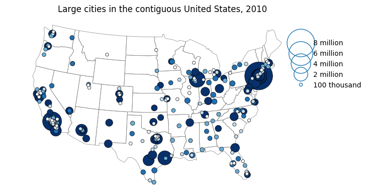
Double visual variable pointplot¶

# Load the data (uses the `quilt` package).
import geopandas as gpd
from quilt.data.ResidentMario import geoplot_data

continental_cities = gpd.read_file(geoplot_data.usa_cities()).query('POP_2010 > 100000')
continental_usa = gpd.read_file(geoplot_data.contiguous_usa())


# Plot the figure.
import geoplot as gplt
import geoplot.crs as gcrs
import matplotlib.pyplot as plt

poly_kwargs = {'linewidth': 0.5, 'edgecolor': 'gray', 'zorder': -1}
point_kwargs = {'linewidth': 0.5, 'edgecolor': 'black', 'alpha': 1}
legend_kwargs = {'bbox_to_anchor': (0.9, 0.9), 'frameon': False}

ax = gplt.polyplot(continental_usa,
                   projection=gcrs.AlbersEqualArea(central_longitude=-98, central_latitude=39.5),
                   **poly_kwargs)

gplt.pointplot(continental_cities, projection=gcrs.AlbersEqualArea(), ax=ax,
               scale='POP_2010', limits=(1, 80),
               hue='POP_2010', cmap='Blues',
               legend=True, legend_var='scale',
               legend_values=[8000000, 6000000, 4000000, 2000000, 100000],
               legend_labels=['8 million', '6 million', '4 million', '2 million', '100 thousand'],
               legend_kwargs=legend_kwargs,
               **point_kwargs)

plt.title("Large cities in the contiguous United States, 2010")
plt.savefig("largest-cities-usa.png", bbox_inches='tight', pad_inches=0.1)