Imputation of quadratic terms

Imputes incomplete variable that appears as both main effect and quadratic effect in the complete-data model.

mice.impute.quadratic(y, ry, x, wy = NULL, ...)

Arguments

y	Vector to be imputed
ry	Logical vector of length `length(y)` indicating the the subset `y[ry]` of elements in `y` to which the imputation model is fitted. The `ry` generally distinguishes the observed (`TRUE`) and missing values (`FALSE`) in `y`.
x	Numeric design matrix with `length(y)` rows with predictors for `y`. Matrix `x` may have no missing values.
wy	Logical vector of length `length(y)`. A `TRUE` value indicates locations in `y` for which imputations are created.
...	Other named arguments.

Value

Vector with imputed data, same type as y, and of length sum(wy)

Details

This function implements the "polynomial combination" method. First, the polynomial combination \(Z = Y \beta_1 + Y^2 \beta_2\) is formed. \(Z\) is imputed by predictive mean matching, followed by a decomposition of the imputed data \(Z\) into components \(Y\) and \(Y^2\). See Van Buuren (2012, pp. 139-141) and Vink et al (2012) for more details. The method ensures that 1) the imputed data for \(Y\) and \(Y^2\) are mutually consistent, and 2) that provides unbiased estimates of the regression weights in a complete-data linear regression that use both \(Y\) and \(Y^2\).

Note

There are two situations to consider. If only the linear term Y is present in the data, calculate the quadratic term YY after imputation. If both the linear term Y and the the quadratic term YY are variables in the data, then first impute Y by calling mice.impute.quadratic() on Y, and then impute YY by passive imputation as meth["YY"] <- "~I(Y^2)". See example section for details. Generally, we would like YY to be present in the data if we need to preserve quadratic relations between YY and any third variables in the multivariate incomplete data that we might wish to impute.

Author

Gerko Vink (University of Utrecht), g.vink@uu.nl

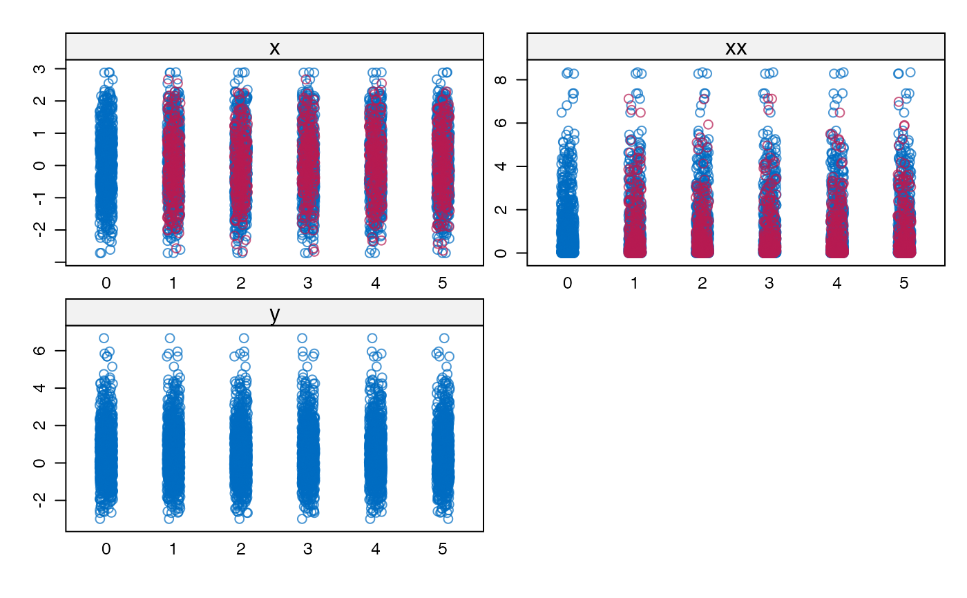
Examples

require(lattice)
#> Loading required package: lattice

# Create Data
B1 <- .5
B2 <- .5
X <- rnorm(1000)
XX <- X^2
e <- rnorm(1000, 0, 1)
Y <- B1 * X + B2 * XX + e
dat <- data.frame(x = X, xx = XX, y = Y)

# Impose 25 percent MCAR Missingness
dat[0 == rbinom(1000, 1, 1 - .25), 1:2] <- NA

# Prepare data for imputation
ini <- mice(dat, maxit = 0)
meth <- c("quadratic", "~I(x^2)", "")
pred <- ini$pred
pred[, "xx"] <- 0

# Impute data
imp <- mice(dat, meth = meth, pred = pred)
#> 
#>  iter imp variable
#>   1   1  x  xx
#>   1   2  x  xx
#>   1   3  x  xx
#>   1   4  x  xx
#>   1   5  x  xx
#>   2   1  x  xx
#>   2   2  x  xx
#>   2   3  x  xx
#>   2   4  x  xx
#>   2   5  x  xx
#>   3   1  x  xx
#>   3   2  x  xx
#>   3   3  x  xx
#>   3   4  x  xx
#>   3   5  x  xx
#>   4   1  x  xx
#>   4   2  x  xx
#>   4   3  x  xx
#>   4   4  x  xx
#>   4   5  x  xx
#>   5   1  x  xx
#>   5   2  x  xx
#>   5   3  x  xx
#>   5   4  x  xx
#>   5   5  x  xx

# Pool results
pool(with(imp, lm(y ~ x + xx)))
#> Class: mipo    m = 5 
#>          term m    estimate         ubar            b            t dfcom
#> 1 (Intercept) 5 -0.05601439 0.0017416853 1.282091e-04 0.0018955363   997
#> 2           x 5  0.44710524 0.0010866872 7.756583e-05 0.0011797662   997
#> 3          xx 5  0.52453983 0.0006169592 7.281374e-05 0.0007043356   997
#>         df        riv     lambda        fmi
#> 1 364.8662 0.08833452 0.08116486 0.08616034
#> 2 377.7501 0.08565390 0.07889614 0.08373450
#> 3 200.2092 0.14162442 0.12405518 0.13267630

# Plot results
stripplot(imp)
plot(dat$x, dat$xx, col = mdc(1), xlab = "x", ylab = "xx")
cmp <- complete(imp)
points(cmp$x[is.na(dat$x)], cmp$xx[is.na(dat$x)], col = mdc(2))