Overview
Chapter 2 is about Abstraction. It concerns how we model and formulate a problem using specific mathematical models. Abstraction is powerful. It begins with identification of a few main entities from the problem, and continues to characterize their relationships. Then we focus on the study of these interconnected entities as a pure mathematical system. Consequences can be analytically established within this abstracted framework, while a phenomenon in a concerned context could be identified as special instances, or manifestations, of the abstracted model. In other words, by making abstraction of a real-world problem, we free ourselves from the application context that is usually unbounded and not well defined.
People often adopt a blackbox view of a real-world problem, as shown in Figure 2. There is one (or more) key performance metrics of the system, called the output variable5 Denoted as \(y\), e.g., the yield of a chemical process, the mortality rate of an ICU, the GDP of a nation, etc., and there is a set of input variables6 Denoted as \(x_{1}, x_{2}, \ldots, x_{p}\); also called predictors, covariates, features, and, sometimes, factors. that may help us predict the output variable. These variables are the few main entities identified from the problem, and how the input variables impact the output variable is one main type of relationship we develop models to characterize.
Figure 2: The blackbox nature of many data science problems

These relationships are usually unknown, due to our lack of understanding of the system. It is not always plausible or economically feasible to develop a Newtonian style characterization of the system7 I.e., using differential equations.. Thus, statistical models are needed. They collect data from this blackbox system and build models to characterize the relationship between the input variables and the output variable. Generally, there are two cultures for statistical modeling8 Breiman, L., * Statistical Modeling: The Two Cultures,* Statistical Science, Volume 16, Issue 3, 199-231, 2001.: One is the data modeling culture , while another is the algorithmic modeling culture . Linear regression models are examples of the data modeling culture; decision tree models are examples of the algorithmic modeling culture.
Two goals are shared by the two cultures: (1) to understand the relationships between the predictors and the output, and (2) to predict the output based on the predictors. The two also share some common criteria to evaluate the success of their models, such as the prediction performance. Another commonality they share is a generic form of their models
\[\begin{equation} y=f(\boldsymbol{x})+\epsilon, \tag{1} \end{equation}\]
where \(f(\boldsymbol{x})\) reflects the signal part of \(y\) that can be ascertained by knowing \(\boldsymbol{x}\), and \(\epsilon\) reflects the noise part of \(y\) that remains uncertain even when we know \(x\). To better illustrate this, we could annotate the model form in Eq. (1) as9 An interesting book about the antagonism between signal and noise: Silver, N., The Signal and the Noise: Why So Many Predictions Fail–but Some Don’t, Penguin Books, 2015. The author’s prediction model, however, failed to predict Donald Trump’s victory of the 2016 US Election.
\[\begin{equation} \underbrace{y}_{data} = \underbrace{f(\boldsymbol{x})}_{signal} + \underbrace{\epsilon}_{noise}, \tag{2} \end{equation}\]
The two cultures differ in their ideas about how to model these two parts. A brief illustration is shown in Table 1.
Table 1: Comparison between the two cultures of models
| \(f(\boldsymbol{x})\) | \(\epsilon\) | Ideology | |
|---|---|---|---|
| Data Modeling | Explicit form (e.g., linear regression). | Statistical distribution (e.g., Gaussian). | Imply Cause and effect; uncertainty has a structure. |
| Algorithmic Modeling | Implicit form (e.g., tree model). | Rarely modeled as structured uncertainty; taken as meaningless noise. | More focus on prediction; to fit data rather than to explain data. |
An illustration of the data modeling, using linear regression model , is shown in Figure 3. To develop such a model, we need efforts in two endeavors: the modeling of the signal, and the modeling of the noise (also called errors). It was probably the modeling of the errors, rather than the modeling of the signal, that eventually established a science: Statistics10 Errors, as the name suggests, are embarrassment to a theory that claims to be rational. Errors are irrational, like a crack on the smooth surface of rationality. But rationally, if we could find a law of errors, we then find the law of irrationality. With that, once again rationality trumps irrationality, and the crack is sealed..
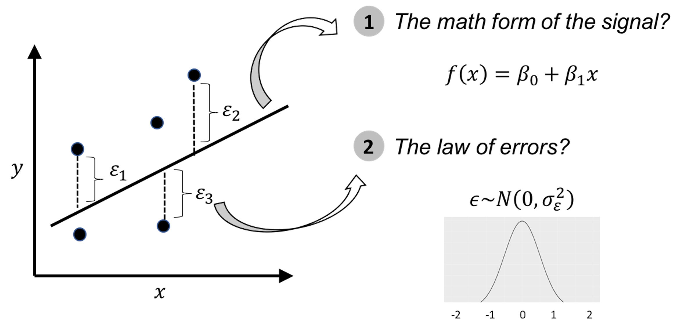
Figure 3: Illustration of the ideology of data modeling, i.e., data is used to calibrate, or, estimate, the parameters of a pre-specified mathematical structure
One only needs to take a look at the beautiful form of the normal distribution (and notice the name as well) to have an impression of its grand status as the law of errors. Comparing with other candidate forms that historically were its competitors, this concentrated, symmetrical, round and smooth form seems a more rational form that a law should take, i.e., see Figure 4.
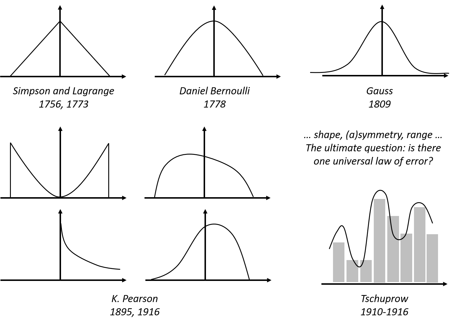
Figure 4: Hypothesized laws of errors, including the normal distribution (also called the Gaussian distribution, developed by Gauss in 1809) and some of its old rivalries
The \(\epsilon\) in Eq. (1) is often called the error term , noise term, or residual term . \(\epsilon\) is usually modeled as a Gaussian distribution with mean as \(0\). The mean has to be \(0\); otherwise, it contradicts with the name error. \(f(\boldsymbol{x})\) is also called the model of the mean structure11 To see that, notice that \(\mathrm{E}{(y)} = \mathrm{E}{[f(\boldsymbol{x}) + \epsilon]} = \mathrm{E}{[f(\boldsymbol{x})]} + \mathrm{E}{[\epsilon]}\). Since \(\mathrm{E}{(\epsilon)} = 0\) and \(f(\boldsymbol{x})\) is not a random variable, we have \(\mathrm{E}{(y)} = f(\boldsymbol{x})\). Thus, \(f(\boldsymbol{x})\) essentially predicts the mean of the output variable..