--snap-max-dist to snap distant quakes to the nearest prefecture instead, or --no-snap to drop every offshore point. magnitude vs felt_reports is almost perfectly correlated (r=0.95); magnitude and felt_reports are right-skewed with flagged outliers; and the magnitude-over-time trend spikes during a September aftershock sequence. --bivariate adds an NMI association heatmap spanning every column type, not just the continuous-numeric ones the Pearson heatmap covers — it surfaces depth_km and felt_reports as strongly associated with the timestamp column (NMI=0.93 and 0.89), a temporal-clustering signal (the same September aftershock sequence) a Pearson matrix restricted to numeric pairs alone cannot express against a date column. Coordinate columns are shown on the map only, not re-charted as distributions. Rendered with the built-in plotly_dark theme.qsv viz smart seismic_events.csv --smarter --bivariate --theme plotly_dark \
--grid-cols 3 --geojson japan_prefectures.geojson -o smart_data_schematic_smarter_geospatial.htmlqsv viz smart HTML output the spatial-extent label calls them out — Colorado, United States — 4 outliers (Wyoming, Kansas & Nebraska) — while strays within the core's own jurisdiction are folded back in silently instead. Each stop also carries delivery attributes (packages, weight_kg, distance_km, delivery_minutes, a vehicle class and a delivered_date), so beyond the map the auto-profiler fills the Data Schematic out with box plots, frequency bars, a correlation heatmap, the strongest-pair scatter (packages vs weight_kg) and a delivered-over-time trend — all without --smarter.qsv viz smart delivery_stops.csv -o smart_data_schematic_geographic_outliers.htmlqsv viz smart sales_sample.csv --hierarchy-style sunburst --max-charts 8 \
-o smart_data_schematic.htmlqsv viz smart sales_sample.csv --dictionary sales_kpi_dict.schema.json \
-o smart_data_schematic_kpi_gauges_target_delta.htmlqsv viz smart customer_spend.csv --smarter --max-charts 8 -o smart_data_schematic_smarter.htmlmedical_payment and total_patients per provider. These are additive amounts across comparable units, so --smarter recognizes them as inequality measures and adds a Lorenz curve for each (Gini 0.65 / 0.61) — the further the curve bows below the diagonal, the more concentrated the payments. The distribution boxes are skew-aware: a heavily right-skewed money column would squash a linear box into a sliver against its largest values, so viz smart draws it on a log axis instead, keeping the median and quartiles legible.qsv viz smart cms_medicare_providers.csv --smarter -o smart_data_schematic_smarter_gini_lorenz_inequality_log_skew_boxes.htmlonboarding_funnel_dict.schema.json (x-qsv.relationships, kind: "pipeline"); which columns are stages, and in which direction, is semantics rather than a statistic, so the panel is only ever drawn from an explicit declaration — never guessed from column names.Here the stages genuinely nest: every row is a strict subset of the one before it, and so are the totals. That is what earns a funnel, whose band widths are a containment claim — plotly computes the stage-to-stage conversion from the bar values themselves (
100% → 41% → 54% → 46%), so the percentages can never drift from the bands. Compare the next figure, where the same kind of declaration over non-nesting totals is drawn as a bridge instead.qsv viz smart onboarding_funnel.csv --dictionary onboarding_funnel_dict.schema.json \
-o smart_data_schematic_dictionary_declared_pipeline_funnel.htmlflat run = 60% zeros, not small values. That long flat opening run is not a mass of small projects — it is the projects with nothing committed or spent yet, a funding-pipeline stage rather than a have-not population. Every Lorenz panel also carries the unit caveat, because a Gini across units as unlike a subway extension and a playground resurfacing is close to tautological and must not be read as inequity.It also carries the pipeline bridge, declared by
nyc_capital_projects_dict.schema.json as an x-qsv.relationships entry of kind: "pipeline". Which columns are stages, and in which direction, is semantics rather than a statistic, so the panel is only ever drawn from an explicit declaration — never guessed from column names.The declaration says these columns are one pipeline; it cannot say that they nest, and that is measured. Here they do not: spent totals 2.9× committed, because the three are independent aggregates on different bases —
totalplannedcommit is allocated in the Capital Commitment Plan, while the other two are sums within the City's budget. A funnel's band widths are a containment claim, so drawing one would render a band wider than the one above it — an hourglass asserting the opposite of the numbers, which no caption can retract. So viz smart keeps the declaration and changes the form: it bridges the signed gap between consecutive totals, naming each step as the arithmetic difference it is (Committed − Planned), never as a flow. Declared order is still never re-sorted by size, and the subtitle says why the form changed: stages do not nest — bridged, not funnelled.qsv viz smart nyc_capital_projects.csv --smarter --dictionary nyc_capital_projects_dict.schema.json \
-o smart_data_schematic_smarter_zero_inflated_capital_pipeline.htmlqsv viz bar sales_sample.csv --x region --y revenue --agg sum \
-o bar.html--slider: each distinct satisfaction rating (1–5) becomes an animation frame, with a ▶ Play/⏸ Pause button and a scrub slider to step through them (Gapminder-style). Axis ranges are pinned across frames so the bars stay comparable frame to frame instead of rescaling. --slider also works on line and scatter, may be split into animated traces with --series, and can accumulate with --slider-cumulative.qsv viz bar sales_sample.csv --x product_category --y revenue \
--agg sum --slider satisfaction -o bar_animated_slider.htmlqsv viz line stock_prices.csv --x date --y close -o line.htmlqsv viz scatter sales_sample.csv --x units_sold --y revenue -o scatter.htmlqsv viz scatter sales_sample.csv --x units_sold --y revenue --size shipping_cost \
--color profit_margin_pct -o scatter_bubble.html--slider supplies the time axis, --series the entity (one colored bubble per region) and --size the third data variable (population). Each region traces a path through the gdp/wellbeing space as the animation plays (▶ Play/⏸ Pause + a scrub slider), with axes pinned across frames and bubble sizes scaled once over every frame so they stay comparable throughout. Each region×month cell collapses to one bubble via --agg (mean by default). This is the same chart viz smart auto-selects (see the last figure), but requested explicitly — so it draws sparse entities too, noting the gaps on stderr instead of dropping them.qsv viz scatter regions_growth.csv --x gdp_index --y wellbeing_index \
--size population_m --series region --slider month_date -o scatter_gapminder_bubble_animation.htmlqsv viz scatter3d sales_sample.csv --x units_sold --y revenue \
--z shipping_cost --color profit_margin_pct -o scatter3d.htmlqsv viz histogram sales_sample.csv --x unit_price -o histogram.htmlqsv viz box sales_sample.csv --y revenue -o box.htmlqsv viz box sales_sample.csv --y revenue --x region --box-points all \
-o box_grouped.htmlqsv viz violin sales_sample.csv --y revenue --x region -o violin.htmlqsv viz pie sales_sample.csv --x product_category --y revenue \
--donut -o pie_donut.htmlviz smart detects automatically.qsv viz funnel signup_funnel.csv --x stage --y users -o funnel.htmlqsv viz heatmap sales_sample.csv -o heatmap_correlation.htmlqsv viz scatter sales_sample.csv --x discount_pct --y profit_margin_pct \
-o scatter_correlated_pair.htmlqsv viz contour sales_sample.csv --x units_sold --y revenue --bins 20 \
-o contour.htmlqsv viz heatmap sales_sample.csv --x region --y product_category \
--z revenue -o heatmap_pivot.htmlqsv viz candlestick stock_prices.csv --x date --ohlc-open open \
--high high --low low --close close -o candlestick.htmlqsv viz ohlc stock_prices.csv --x date --ohlc-open open --high high \
--low low --close close -o ohlc.htmlqsv viz radar product_ratings.csv --cols battery,camera,performance,display,value,design \
--series brand -o radar.htmlqsv viz sankey web_flows.csv --source source --target target \
--value sessions -o sankey.htmlqsv viz treemap customer_spend.csv --cols plan,region --value monthly_spend \
--agg sum -o treemap.htmlqsv viz sunburst sales_sample.csv --cols region,product_category,payment_method \
-o sunburst.htmlqsv viz icicle sales_sample.csv --cols region,product_category,payment_method \
-o icicle.htmlviz smart Data Schematic has no SPLOM panel; it covers the same ground with its correlation heatmap plus the strongest-pair scatter and 3D scatter drill-downs.qsv viz splom sales_sample.csv --cols units_sold,revenue,discount_pct,profit_margin_pct \
-o splom.htmlqsv viz parcats sales_sample.csv --cols region,product_category,payment_method \
-o parcats.htmlqsv viz map quakes.csv --lat lat --lon lon --color magnitude \
--size depth_km -o map.html--color) so stronger quakes glow hotter — hovering a point shows its magnitude, not just the coordinates.qsv viz map quakes.csv --lat lat --lon lon --density --color magnitude \
--style carto-positron -o map_density.htmlqsv viz geo quakes.csv --lat lat --lon lon --color magnitude \
--projection natural-earth -o geo.html--slider steps through the region column, revealing the world's seismicity continent by continent, each region in its own color via --series. With --slider-cumulative the points accumulate as the animation plays (Play/Pause + a scrub slider). Unlike the MapLibre tile map, scattergeo animates natively, so --slider is supported on viz geo — use it instead of viz map for animated point maps.qsv viz geo quakes.csv --lat lat --lon lon --slider region --series region \
--slider-cumulative --projection natural-earth -o geo_animated_slider.htmlqsv viz choropleth country_stats.csv --locations iso3 --value gdp_usd_tn \
--color-scale viridis -o choropleth.html--location-mode usa-states: state codes matched to Plotly's built-in US-state geometry on the token-free albers-usa projection (CONUS + Alaska/Hawaii insets) — no GeoJSON needed. States are colored by renewable-electricity share.qsv viz choropleth us_state_stats.csv --locations state --value renewable_electricity_pct \
--location-mode usa-states -o choropleth_us_states.html--map draws the filled regions on an interactive MapLibre tile basemap (token-free carto-positron) instead of a projection. The regions come from a custom GeoJSON (--geojson local file or URL) matched to the data by --feature-id-key — here the 11 Northeast states with real Census TIGER boundaries, colored by population density. The id lives in the feature's properties (--feature-id-key properties.STUSAB), which is the common real-world case — most published GeoJSON keys its regions there rather than on a top-level id. Density is an intensive quantity, so --agg mean is passed: with one row per region it leaves the values untouched, but it keeps hover from offering a share-of-total percentage — the sum of eleven densities is not a total of anything. The view auto-centers and zooms to the GeoJSON extent (shown full-width so the computed zoom frames the regions as the CLI does — a tile map's zoom is fixed, so a narrow grid cell would crop it).qsv viz choropleth northeast_states.csv --locations state --value people_per_sq_mi \
--agg mean --geojson northeast_states.geojson --feature-id-key properties.STUSAB \
--map --style carto-positron -o choropleth_maplibre_geojson.html--geojson auto reads the county FIPS codes in county_fips, derives the states they name (PA, OH, WV), and fetches just those states' county boundaries from the Census Bureau's TIGERweb service, setting --feature-id-key to properties.GEOID itself. County FIPS and ZIP codes are both 5-digit numerics, so qsv cannot tell them apart by shape — it probes each candidate layer (geometry-free, a few KB) and takes the one the codes actually resolve against, refusing to guess on a tie. Whole states are fetched rather than only the 13 counties named, so the match fraction is scored against a boundary set that was NOT derived from the column being scored. The note beneath the map records the vintage, which matters: Connecticut replaced its 8 counties with 9 planning regions in the 2022 vintages, sharing no GEOID, so append @2021 to pin an older one. Boundaries are cached, so a repeat run makes no network request at all. (Broadband figures here are synthetic.)qsv viz choropleth tristate_county_broadband.csv --locations county_fips \
--value broadband_pct --location-mode geojson-id --geojson auto \
--title 'Household broadband adoption by county (synthetic)' \
-o choropleth_geojson_auto_census_counties.htmlSTATE field, so unlike counties they cannot be state-scoped and are fetched by exact code set, which is what makes the two caveats in the note worth reading. Five of the 132 ZIPs match no ZCTA at all (PO-box-only ZIPs have no tabulation area) and are reported rather than silently dropped. Six more sit far outside the rest — two Florida and two Indiana owner ZIPs, four rows out of 50,013 — and framing to the full extent would render the Pittsburgh cluster as a speck on a map reaching Miami. Those regions are still drawn; they just do not get to decide the frame, and the note says so. A boundary set qsv derived from your codes is not the same as a file you chose, so it does not get the same benefit of the doubt.qsv viz choropleth allegheny_dog_licenses.csv --locations OwnerZip \
--location-mode geojson-id --geojson auto --title 'Allegheny County dog licenses by owner ZIP' \
-o choropleth_geojson_auto_census_zctas_honesty_reporting.htmlqsv viz smart stock_prices.csv --max-charts 8 -o smart_data_schematic_time_series.htmlqsv viz smart us_cities.csv -o smart_data_schematic_per_us_state_choropleth.htmlqsv viz smart customer_spend.csv --dictionary infer -o smart_data_schematic_dictionary_infer_treemap.htmlqsv viz smart sales_sample.csv --dictionary infer --hierarchy-style sunburst \
-o smart_data_schematic_dictionary_infer_sunburst.htmlfitbounds — so the regions are never clipped at the viewport edge — beside the dense natural-earth point map (crimson markers so coastal/island points read against the ocean), plus a six-continent breakdown. A describegpt-inferred Data Dictionary supplies the friendly field labels (e.g. Metropolitan Population (Millions), Average Annual Temperature). The continent column follows the plotly.js geo scope continent vocabulary (Oceania, North America, …). Note: elevation_m is real (GeoNames), while avg_annual_temp_c is a rough synthetic proxy (latitude + elevation-lapse model), so treat it as illustrative. Requires a local LLM; the committed HTML is reused on regen.qsv viz smart world_cities.csv --dictionary infer -o smart_data_schematic_dictionary_infer_world_choropleth.htmlOwnerZip column, so viz smart aggregates licenses per zip and fills the matching Allegheny County zip-boundary polygons from --geojson (--feature-id-key properties.ZIP). The key column is auto-chosen by matching each geo-dimension column's values against the boundary ids — here 118 zips match, from 1 license (rural fringe) to 2,866 in zip 15237 (suburban North Hills). Because the matched regions span a metro-scale extent, the fill lands on an interactive MapLibre tile basemap (token-free carto tiles) rather than the coarse projection basemap used for country/continental choropleths. A curated --dictionary (allegheny_dogs_dict.schema.json) tags OwnerZip as geo.zip_code — the signal that turns a numeric zip code into a choropleth key instead of a frequency bar — and marks _id/DogName as identifiers so they're skipped. This dataset carries no numeric measure, so only the per-zip count map is drawn; a dataset that also tags a measure column (e.g. a sale price) additionally gets a per-zip median-of-measure choropleth beside it. Alongside the map the profiler fills the Data Schematic with LicenseType/Breed/Color frequency bars and, via --bivariate, an NMI association heatmap (LicenseType, Breed & Color; the ranked Top Relationships panel only joins it past 8 associated columns). --dict-info adds a per-panel info icon and a slide-over Data Schematic drawer sourced from the same curated schema, topped by a download row bundling the dictionary, the charted frequency counts and the stats & bivariate sidecars into the HTML itself. Fully deterministic — no LLM needed (the curated dictionary is reviewed and committed, exactly like an --dictionary infer pass would produce).qsv viz smart allegheny_dog_licenses.csv --smarter --bivariate \
--dict-info --dictionary allegheny_dogs_dict.schema.json --geojson allegheny_zip_boundaries.geojson \
--feature-id-key properties.ZIP -o smart_data_schematic_smarter_curated_dictionary_region_code_zip_choropleth.htmlx-qsv.denominator: {"column": "population", "level": "geo.county"} on the region column in the curated dictionary. The level declares which geography those values describe, and is checked against the region column's own concept: a denominator describing a different geography from the one the map is keyed by is refused rather than charted. The case that motivates it is a coarser one — state populations against county regions — which is constant within each region and positive, so it passes every data-derived check while charting a confidently wrong rate. A hint that declares no level still charts, and says so in its subtitle. --denominator-key properties.POP2020 would instead read it from the boundary file, and viz choropleth --denominator turns a standalone map into a rate map. The scale (per 1,000 / 10,000 / 100,000) is chosen from the MEDIAN rate, so one freak district can't rescale the map, and hover keeps the raw count and the named denominator beside the rate — with no share-of-total line, since a rate is intensive. A region map with no denominator available instead says so in its subtitle. The districts are synthetic, laid out on a grid at the geographic centre of the contiguous US; only the shape of the fallacy is real.qsv viz smart district_requests.csv --dict-info --dictionary district_requests_dict.schema.json \
--geojson district_boundaries.geojson -o smart_data_schematic_denominator_aware_region_rate.html--denominator census@2024 fetches ACS 5-year total population (B01003) from the Census Data API for the 210 matched GEOIDs and stamps the release beneath the map — Denominator: ACS 2020–2024 5-yr (B01003) — because a rate means something different against a different release; results cache under ~/.qsv-cache, so a repeat run makes no request. Boundaries are committed (tristate_counties.geojson, TIGERweb at maxAllowableOffset=0.001) rather than fetched with --geojson auto, whose county geometry is generalized more finely (0.0005°, ~50 m): viz smart embeds the geometry once PER TRACE and this figure has two, so the coarser committed file keeps the page small. The curated --dictionary tags only county_fips as geo.county_fips — concepts come from a data dictionary, and a stats-only run has no choropleth candidates at all. Note the county names carry their state: 30 of the 175 distinct names in these three states belong to more than one county (Mercer and Wayne to all three), so a bare name would silently sum them in the frequency bar. The incidents are SYNTHETIC, generated by gen_tristate_county_incidents.py with a per-capita rate deliberately anti-correlated with population; the counties, boundaries and denominator are all real.qsv viz smart tristate_county_incidents.csv --dict-info --dictionary tristate_county_incidents_dict.schema.json \
--geojson tristate_counties.geojson --feature-id-key properties.GEOID \
--denominator census@2024 -o smart_data_schematic_denominator_aware_region_rate_real_counties.html--denominator census@2024 fetches ACS 5-year total population (B01003) from the Census Data API and stamps the release beneath the map — Denominator: ACS 2020–2024 5-yr (B01003). Unlike its neighbour this figure keys on county names with --geojson auto, which fetches the boundaries and canonicalizes the names to Census GEOIDs so the fetched population keys onto them — so there is no FIPS column and no committed boundary file. ⚠️ Read the rate map as service reach as much as need, and the map says so itself: the darkest county on it is McKean, at 2 requests against 39,904 residents — 0.05 per 1,000, where the next-lowest county (Elk) is 12.3, some 245 times higher. Nobody believes McKean County has no hardship; it sits at the edge of this call center's intake, so the figure is measuring who dials 2-1-1, not who needs it. A per-capita map inherits whatever the numerator was actually counting. The upstream feed's zip_code is dropped rather than mis-tagged (a second geo concept would create a competing choropleth candidate), and the dataset's OLDER 2020-2023 resource is deliberately not concatenated: 5.4% of its rows carry a pipe-delimited Allegheny County|Westmoreland County multi-county value, and every way of resolving those changes the map.qsv viz smart wpa_211_requests.csv --smarter --bivariate --dict-info \
--dictionary wpa_211_requests_dict.schema.json --geojson auto \
--denominator census@2024 --theme plotly_white --dataset-pid https://data.wprdc.org/dataset/211-requests \
-o smart_data_schematic_real_per_capita_county_rate_wprdc_2_1_1.htmlviz smart draws a ScatterGeo projection basemap (which animates natively, unlike a MapLibre tile map) and adds an animated geographic reveal: the points accumulate cumulatively over monthly time buckets (Play/Pause + scrub slider). A city-scale point cloud would stay a static map — the animation only fires for large extents.qsv viz smart world_events_dated.csv -o smart_data_schematic_animated_geo_world_events.htmlregion) + a measure pair (gdp_index vs wellbeing_index) + a monthly date drive a Gapminder-style animated bubble chart — one bubble per region, each tracing a distinct curved path through the measure space over time, sized by per-cell record count and colored by region (Play/Pause + scrub slider, legend of regions). Strict quality gates (min rows per cell, near-complete per-entity panel) keep it a real drift story rather than noisy jitter.qsv viz smart regions_growth.csv -o smart_data_schematic_gapminder_bubble_regions_growth.htmlqsv viz smart Data Schematic over real Pittsburgh 311 service requests from the Western Pennsylvania Regional Data Center (WPRDC). The Data Schematic bins each request's lat/lon by point-in-polygon into Pittsburgh's neighborhood polygons (--geojson pittsburgh-neighborhoods, a QSV_GEOJSON_SHORTCUTS alias for --geojson pittsburgh_neighborhoods.geojson --feature-id-key properties.hood; no geocoding); a curated --dictionary (pitt311data.schema.json) tags identifier/code columns and supplies friendly field labels, and --dict-info renders that dictionary as its own in-page Data Schematic tab (with a hover/click info icon on every panel title). --smarter enriches the stats cache (moarstats --advanced) and --bivariate adds the NMI association heatmap plus the ranked top-relationships panel, while --dataset-pid adds a clickable citation link back to the source dataset. The standalone page is a ~10.7 MB self-contained Data Schematic — too large to embed inline — so this is a screenshot: click it to open the fully interactive Data Schematic in a new window.qsv viz smart pittsburgh_311.tsv --smarter --dictionary pitt311data.schema.json \
--dict-info --bivariate -o pitt311data.html --geojson pittsburgh-neighborhoods \
--dataset-pid https://data.wprdc.org/dataset/pittsburgh-311-data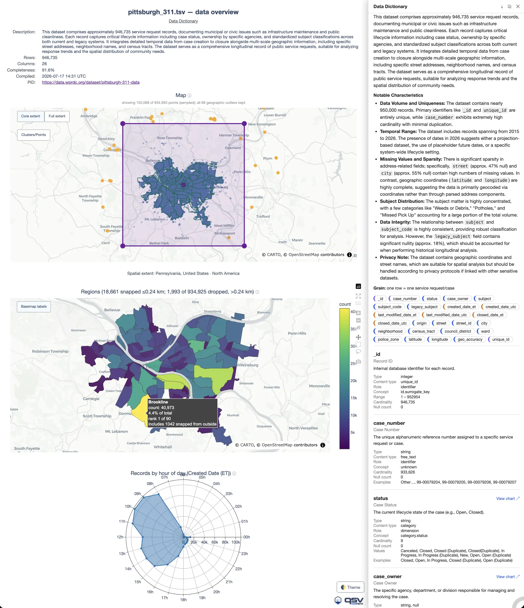
viz smart draws the filled regions on an interactive MapLibre tile basemap (token-free carto tiles, fine street/coastline detail) instead of the coarse projection basemap it uses for country/continental choropleths. The leading point map flags bad-geocode outliers (here, 9 in Pennsylvania): a nice illustration of the hover's value — for a stray PA point, the tooltip shows the record's own Incident City: NEW YORK right above its reverse-geocoded Pennsylvania, United States, so a real Manhattan complaint saddled with corrupt coordinates is self-evident at a glance. --smarter runs moarstats --advanced to enrich the stats cache, and a committed --dictionary (nyc311_dict.schema.json — a Data Dictionary generated for this dataset, then reviewed and committed alongside it) tags the record's identifier columns (Unique Key, BBL) so they're skipped rather than charted as quantities, labels the State-Plane coordinates as coordinate dimensions, and supplies friendly names (e.g. Complaint Creation Date, Resolution Deadline), so the profiler treats a service-request log as volume-and-category data. Alongside the maps the auto-profiler fills the Data Schematic with frequency bars, an hour-of-day seasonality profile, a time trend, a parallel-categories (parcats) flow over 3-4 associated categorical columns (co-occurrence ribbons, auto-chosen over a nested treemap/sunburst for this many-to-many set). New here is an auto-selected, colored Sankey flow (Agency Code → Source Channel Type): it traces how each city agency's complaints arrive by channel, the thickest ribbons being HPD → PHONE (1,426) and NYPD → PHONE (1,348). --bivariate adds an NMI association heatmap across 29 of the charted columns plus a ranked Top Relationships panel — a horizontal multivariate lollipop where each dot's position is the pair's NMI on a value axis zoomed to the shown band (so near-ceiling associations separate instead of crushing together at 1.0), its size encodes co-occurrence support, and an amber dot flags a nonlinear pair. The top pair is a purely categorical one a Pearson-only heatmap could never surface, since neither column is numeric: Borough × Park Borough (NMI=1.0). The ranking is support-weighted: a pair only qualifies when its co-occurring row count is at least 10% of the best-supported pair's, so a technically-perfect NMI from two sparsely-populated columns can't crowd out a more broadly meaningful one. Below the top pair, the ranking surfaces the dataset's redundant columns — the same street recorded twice (Cross Street 1/2 × Intersection Street 1/2) and a code/name lookup (Agency × Agency Name) — exactly the columns a curated dictionary or a select would fold together. No pair here is nonlinear, so every dot keeps the default color. --dict-info adds a per-panel info icon and a slide-over Data Schematic drawer sourced from the same committed schema, topped by a download row that bundles the dictionary as JSON Schema, the frequency counts the panels actually charted, and the stats & bivariate sidecars this run was built from — every file carried inside the HTML, so anyone you send the Data Schematic to can save them. The run stays fully deterministic and offline: because the dictionary is committed, --bivariate never triggers a live --dictionary infer pass. The standalone page is a ~4 MB Data Schematic, shown here as a screenshot so the gallery page stays light: click it to open the fully interactive Data Schematic in a new window.qsv viz smart nyc_311.csv --smarter --bivariate --dict-info --dictionary nyc311_dict.schema.json \
--geojson nyc_neighborhoods.geojson -o smart_nyc311.html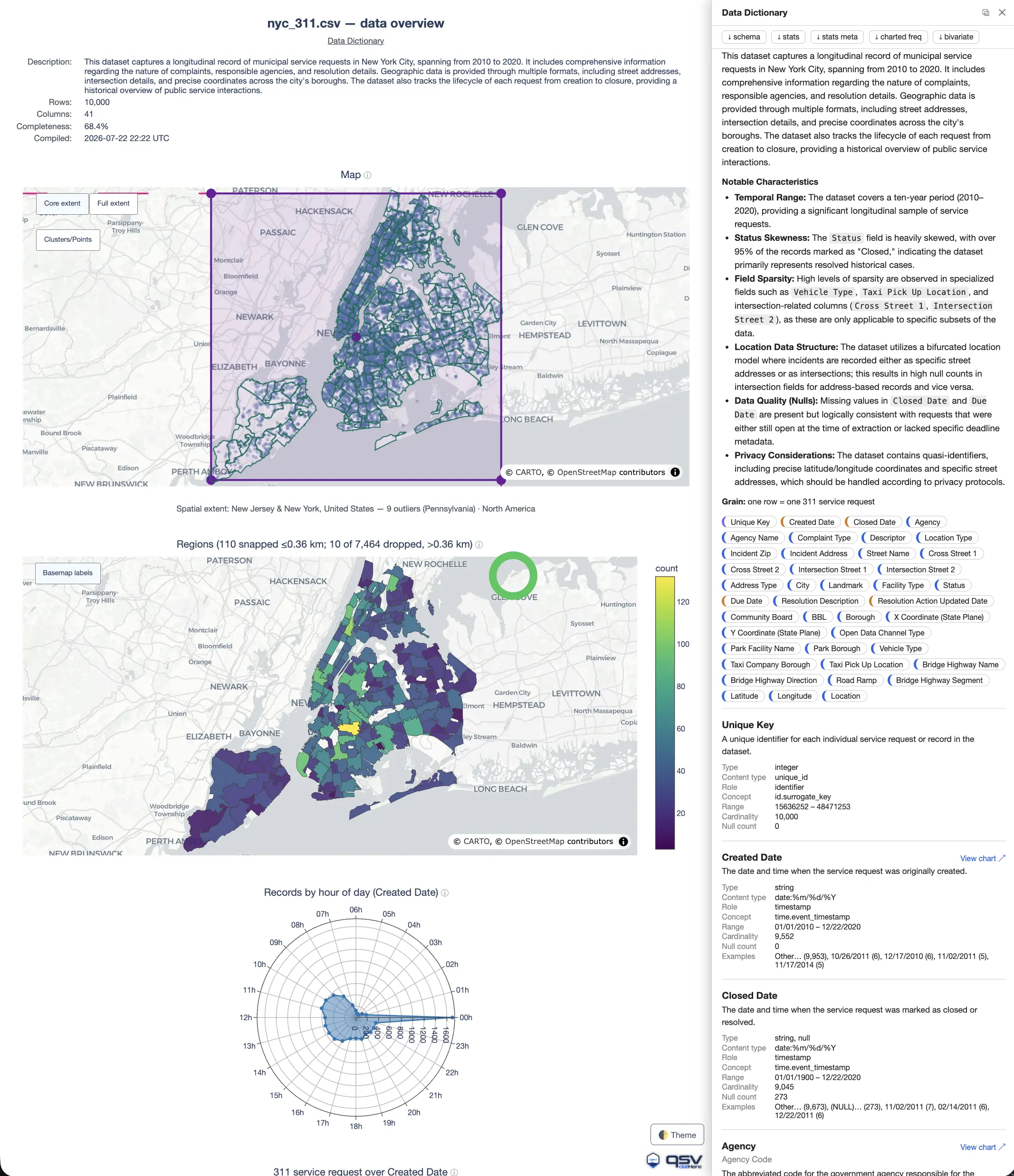
qsv viz smart Data Schematic over a full year of Boston 311 service requests (2025): 267,187 rows x 31 columns, 92.6% complete, from the City of Boston open data portal, profiled into some 30 auto-chosen panels. A dense point map leads, followed by a 25-neighborhood choropleth: each request's coordinates are binned point-in-polygon into Boston's neighborhood boundaries (--geojson with --feature-id-key properties.name, no geocoding) — Dorchester tops it at 38,855 requests (14.7%, rank 1 of 25), and each region's hover reports how many nearby strays were snapped into it. Because the matched regions span a city-scale extent, the fill lands on an interactive MapLibre tile basemap rather than the coarse projection basemap used for country/continental choropleths. Beyond the maps the auto-profiler adds hour-of-day and day-of-week seasonality rings, a case-volume time trend, a parallel-categories flow (Data Source → Subject Area → Fire District → City Council District), a Fire District → City Council District Sankey, the --bivariate NMI association heatmap with its ranked Top Relationships panel, and 23 frequency bars — among them the SLA split (ONTIME 182,145 vs OVERDUE 85,042). --smarter enriches the stats cache (moarstats --advanced), and a committed --dictionary (boston311.schema.json, generated with qsv describegpt --dictionary --two-pass --format jsonschema, then reviewed and committed) supplies the friendly field labels that --dict-info renders as the in-page Data Schematic tab — a hover/click info icon on every panel title, and a download row bundling the dictionary as JSON Schema alongside the stats and charted-frequency sidecars this run was built from. --dataset-pid adds a clickable citation link back to the source dataset. --photos turns the closed_photo column into map imagery: a point that has a photo says so in its hover, and resting on it for two seconds opens the case photo in a small preview beside the marker (nothing is fetched until you dwell, since the images load from a third-party host). Embedding every one of the 264,951 mapped points (all 267,187 records, via QSV_VIZ_MAX_POINTS=300000), plus the first 50,000 rows for the data viewer drawer that the row count's (Preview) link opens, makes this a ~21.9 MB self-contained Data Schematic — too large to embed inline — so this is a screenshot: click it to open the fully interactive Data Schematic in a new window.QSV_VIZ_MAX_POINTS=300000 qsv viz smart boston311-2025.tsv --smarter \
--dictionary boston311.schema.json --dict-info --bivariate --photos \
-o smart_boston_311_2025.html --geojson boston_neighborhood_boundaries.json \
--dataset-pid https://data.boston.gov/dataset/311-service-requests/resource/9d7c2214-4709-478a-a2e8-fb2020a5bb94 \
--feature-id-key properties.name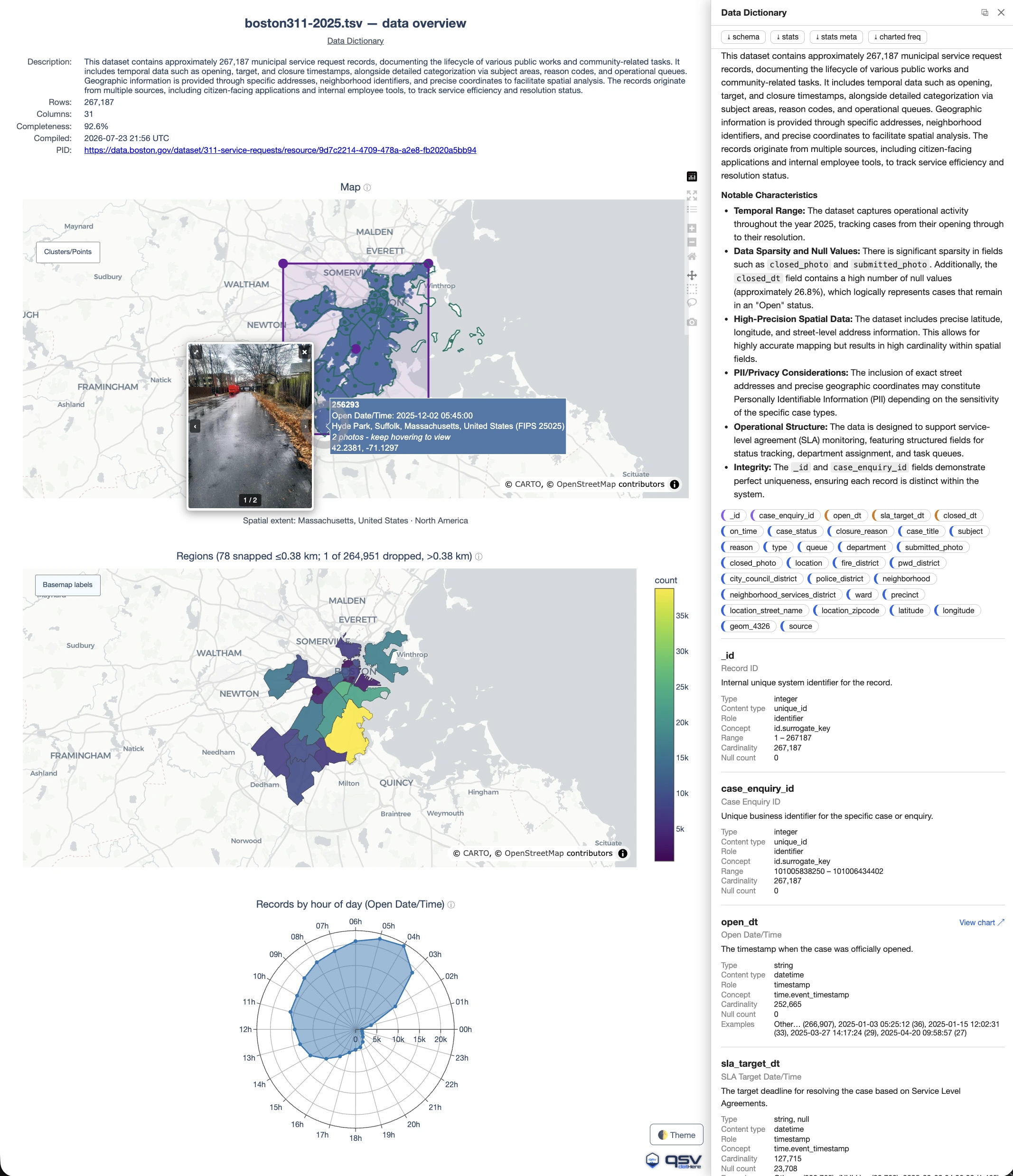
qsv viz smart Data Schematic rendered entirely in Portuguese over four weeks of LPG (GLP) cooking-gas prices — 12,732 rows x 16 columns, 89.1% complete — from Brazil's national open data portal, dados.gov.br. This is the localization showcase: --language pt resolves through the curated pt-BR locale (the bare tag is a registered alias), so every piece of Data Schematic chrome — Descrição, Linhas, Colunas, Completude, Data Schematic, Ver o gráfico — plus the vendored plotly and DataTables locale bundles all render in Portuguese. The input is a semicolon-separated (.ssv) export whose dates are day-first, so QSV_PREFER_DMY=1 makes Data da Coleta parse as DD/MM/YYYY rather than month-first. The auto-profiler leads with a 27-state choropleth (contagem por Estado (Sigla)) drawn on the coarse projection basemap viz smart uses for country-scale extents, followed by a day-of-week radar over the collection date and a price time trend. --bivariate adds the NMI association panels (and implicitly forces --smarter, so the stats cache is enriched by moarstats --advanced), while a committed --dictionary supplies the friendly Portuguese field labels that --dict-info renders as the in-page Data Schematic tab. Neither the .ssv export nor brazil_geo.json is committed here, so this page is reused as-is. The standalone Data Schematic is a ~18 MB self-contained page — too large to embed inline — so this is a screenshot: click it to open the fully interactive Data Schematic in a new window.QSV_PREFER_DMY=1 qsv viz smart ultimas-4-semanas-glp.ssv --smarter \
--dictionary ultimas-4-semanas-glp.schema.json --dict-info --bivariate \
-o smart-brazil-lpg-4-semanas.html --geojson brazil_geo.json \
--language pt --dataset-pid https://dados.gov.br/dados/conjuntos-dados/serie-historica-de-precos-de-combustiveis-e-de-glp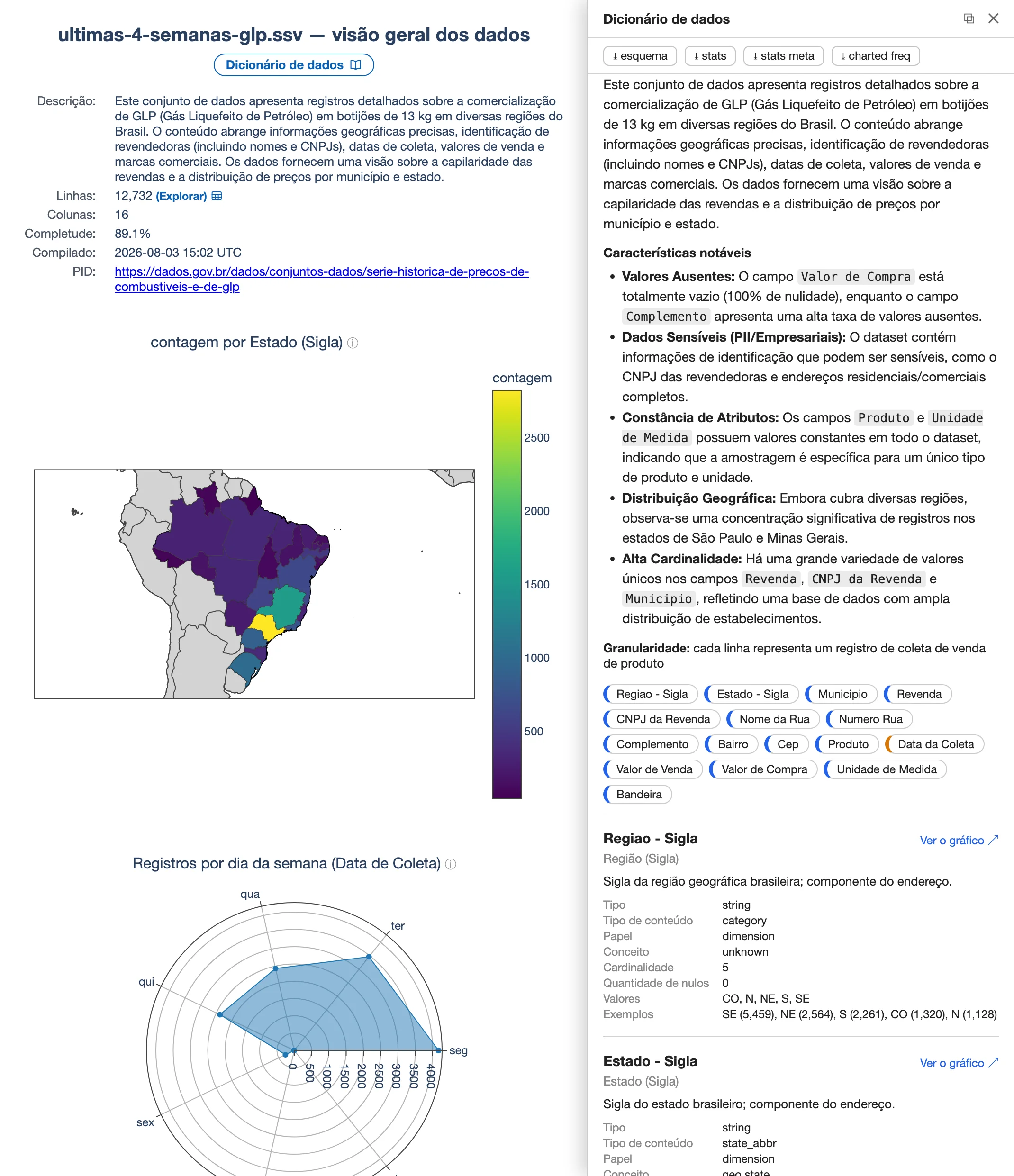
qsv viz smart Data Schematic rendered entirely in Spanish (--language es) over PM10 / PM2.5 particulate measurements recorded at Colombian monitoring stations between 2011 and 2024 — 8,842 rows x 25 columns, 100% complete. A KPI row headlines the totals (19.2M observations, 758k exceedance counts, 182k days with an exceedance), followed by a station point map and a department choropleth (Regiones) that bins each station point-in-polygon into Colombia's department boundaries via --geojson colombia_departments.geojson with --feature-id-key properties.shapeName — 14 stray points are snapped to their nearest department within the auto-derived 35 km cap. Because the matched regions span a country-scale extent the fill lands on an interactive MapLibre tile basemap. The committed --dictionary is hand-tuned, and both edits are load-bearing: Latitud/Longitud carry explicit geo.latitude/geo.longitude concepts because viz's header-name fallback matches only the English lat/latitude/lon/longitude (without them the Data Schematic has no map at all), and only the genuinely additive columns keep role=measure — viz recognises non-additive measures from an English token list, so Spanish Promedio/Mediana/Porcentaje would otherwise be SUMMED into meaningless KPI totals. --bivariate adds the NMI association panels (and implicitly forces --smarter), and --dict-info renders the dictionary as the in-page Data Schematic tab. Regenerate with the committed dictionary, not --dictionary infer. The standalone Data Schematic is a ~5.4 MB self-contained page, shown here as a screenshot so the gallery page stays light: click it to open the fully interactive Data Schematic in a new window.qsv viz smart calidad-aire-pm-colombia.csv --language es --geojson colombia_departments.geojson \
--feature-id-key properties.shapeName --dictionary calidad-aire-pm-colombia.schema.json \
--dict-info --bivariate -o smart-colombia-calidad-aire.html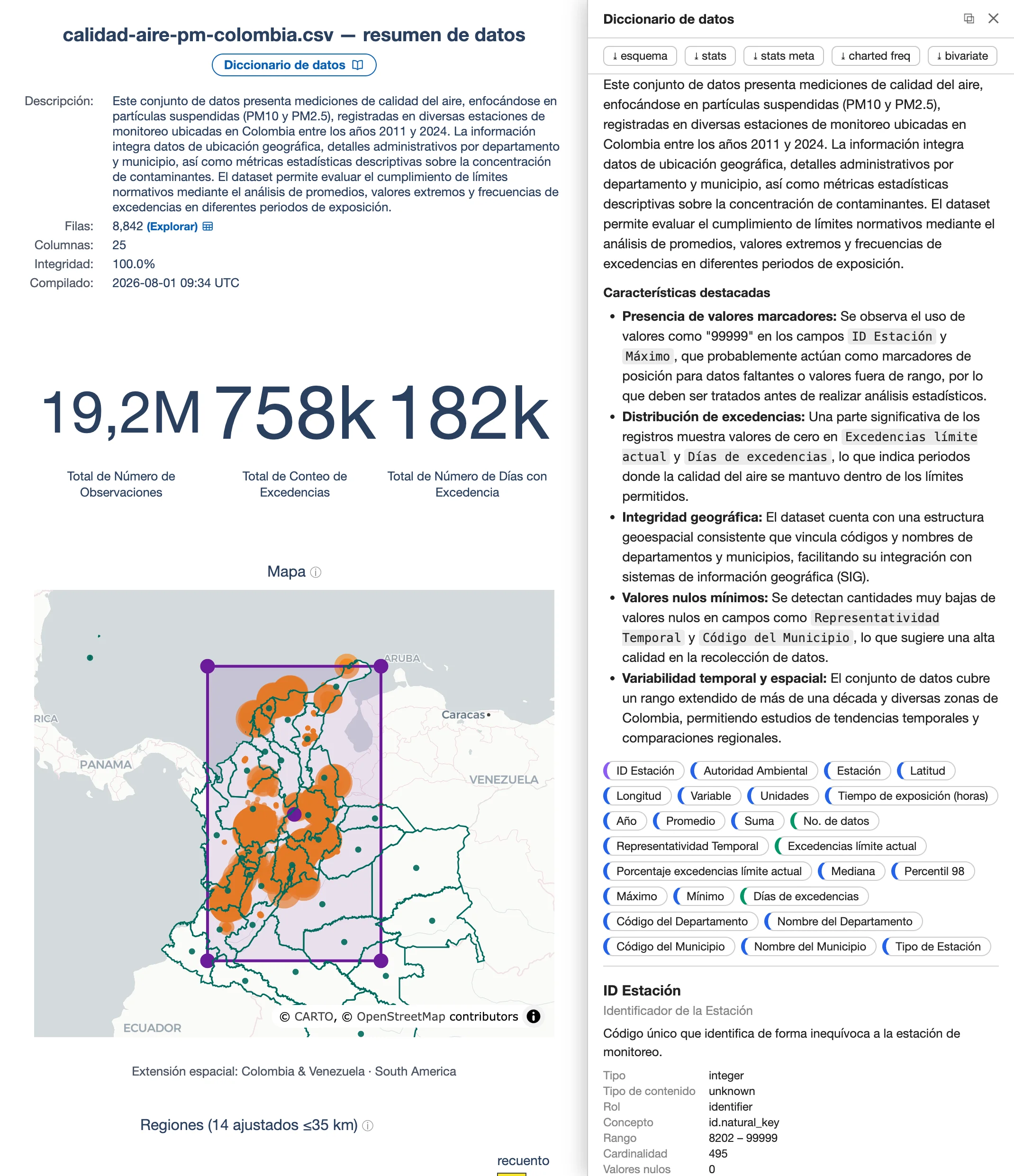
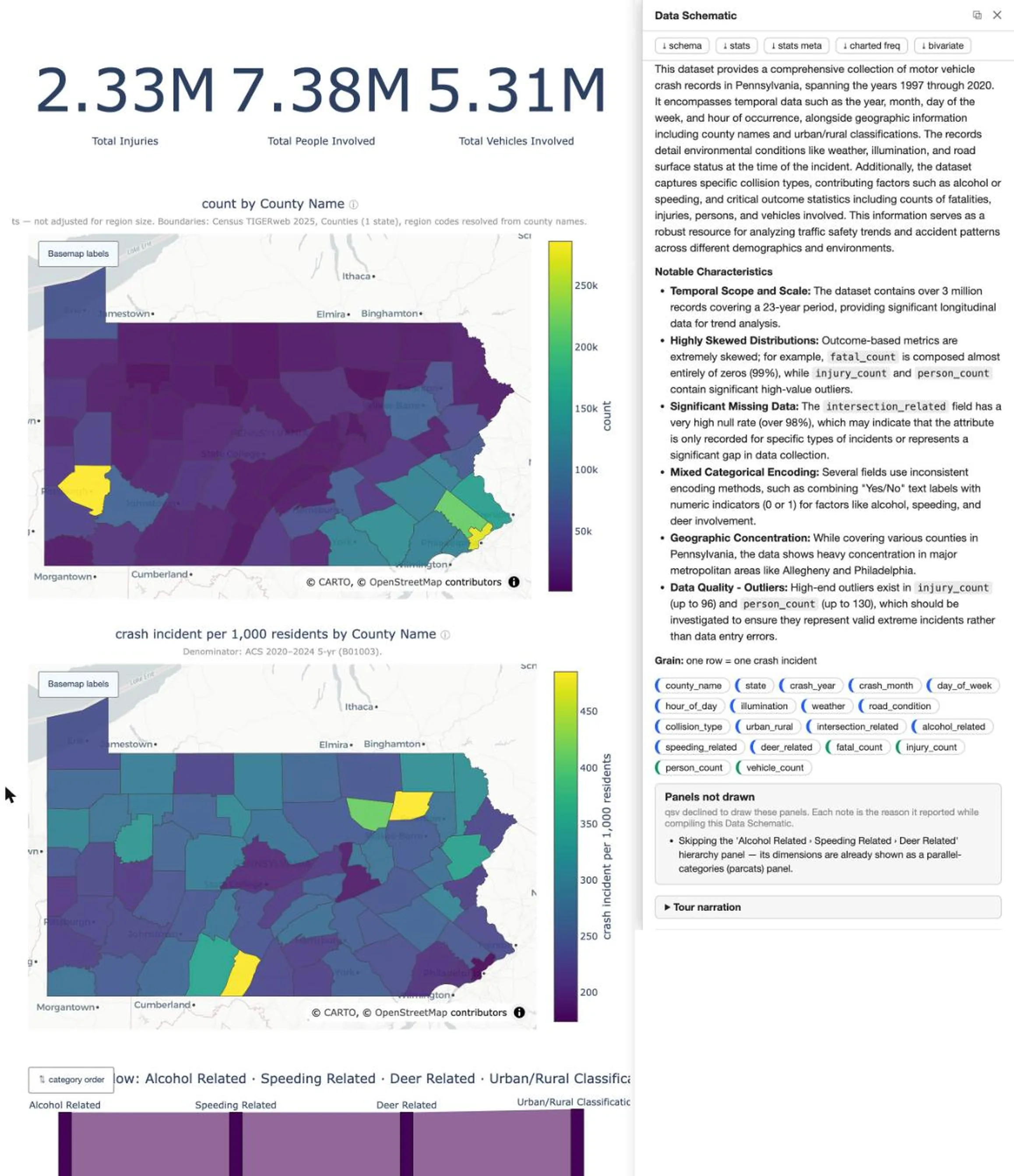
--denominator census figure, and the only one with a light theme (--theme plotly_white). 3,088,272 PennDOT crash records across all 67 Pennsylvania counties (data.pa.gov dc5b-gebx, a 19-column slice of a 219-column table). The dataset title says “CY 1997 - Current” but the data stops at 2020 — the figure is captioned for what is actually in it. --geojson auto does double duty: it fetches the county boundaries from the Census TIGERweb service and canonicalizes the county-name column to Census GEOIDs, which is what lets --denominator census@2024 key fetched ACS population onto the same regions. So the Data Schematic draws each map twice, raw and per capita: the raw count by County Name (labelled “not adjusted for region size”) and crash incident per 1,000 residents beneath it. They tell opposite stories. Allegheny (286,238 crashes) and Philadelphia (274,824) top the count map — which is largely a population map — while on the rate map Philadelphia ranks 67th of 67 (174 per 1,000) and Allegheny 51st (231); rural Wyoming (486) and Fulton (483) lead. Because injury_count is an additive measure, a second pair follows: Injuries by County Name (the per-county total, not a row count) and Injuries per 1,000 residents. Here Philadelphia leads the total (313,927 injuries, ahead of Allegheny's 198,224 despite fewer crashes) yet ranks only 21st per capita (199 per 1,000), while Fulton (329) and Wyoming (318) again top the rate map and Allegheny falls to 56th (160). Two honest caveats the maps cannot state for themselves: the rates are 23-year cumulative, not annual (Wyoming's 486 is ~21 crashes per 1,000 per year), and a per-resident rate under-counts commuter and through-traffic exposure, which is very likely why low-population counties carrying I-80 and I-70 come out on top. The ACS vintage is pinned (census@2024): unpinned, qsv probes the newest published release against today, so a rebuild next year would silently re-vintage every number on this page. This is a screenshot of the standalone, self-contained Data Schematic (~4 MB): click it to open the fully interactive Data Schematic in a new window.qsv viz smart pa_crashes.csv --smarter --dictionary pa_crashes.schema.json \
--dict-info --bivariate --theme plotly_white --geojson auto --denominator census@2024 \
-o smart_pa_crashes.html --dataset-pid https://data.pa.gov/Transportation/Crash-Incident-Details-CY-1997-Current-Annual-Count/dc5b-gebx