## Abstract {#abstract}
Scattering changes the angular momentum exchanged between a bar and resonant orbits. The net effect depends on how the orbits are populated, but local calculations often replace that population with a simple distribution. We test the error introduced by this replacement in a prescribed sweeping-resonance model with additive action diffusion. A Gaussian, an exponential and a reference isochrone distribution are matched in density and slope at the initial resonance. In the tested slice of orbital actions, the Gaussian gives a positive noise-minus-smooth transfer contrast at an early time when the reference distribution gives a negative contrast. At a later time both contrasts are negative, but the Gaussian contrast has 4.7 times the reference magnitude. The exponential closely follows the reference at both times. We explain this difference using a response kernel that separates the dynamics of the orbits from their initial abundance. The kernel also provides a test of population-approximation error. At a second sweep rate, all eight comparisons accepted by this test satisfy the specified 5 per cent accuracy criterion in an independent calculation; four other accurate comparisons are rejected because the test discards signed cancellation. A finite-displacement control reduces the sampling variance for broad populations. These results identify a source of error in finite-time resonance calculations and a way to assess it within the prescribed local model. Their extension to a self-consistent halo remains untested.
[Learn the foundations](https://raw.githubusercontent.com/djova/bar-halo-benchmark/publication-2026-09-24.2/publication/web/learn.md) · [Inspect and reproduce](https://raw.githubusercontent.com/djova/bar-halo-benchmark/publication-2026-09-24.2/publication/web/reproduce.md) · [Claim registry](https://raw.githubusercontent.com/djova/bar-halo-benchmark/publication-2026-09-24.2/publication/web/claims.json) · [Download this article](https://raw.githubusercontent.com/djova/bar-halo-benchmark/publication-2026-09-24.2/publication/web/paper.md)
## Introduction {#previous-work}
A rotating bar continually accelerates and decelerates the particles of its surrounding halo. For most orbits, the phase relative to the bar changes rapidly, and successive torque contributions largely cancel. Near a resonance, that phase changes slowly enough for the torque to accumulate. Some orbits become trapped and oscillate about a preferred phase relative to the bar. The angular momentum exchanged by the population therefore depends on both the response of individual orbits and the number of particles occupying each part of phase space.
Scattering can change this exchange even when it produces only a small change in an orbit's total action. The relevant scale is the width of the resonance. [Hamilton et al. (2023)](https://arxiv.org/abs/2208.03855) showed that diffusion across this width can sustain torque at a stationary bar resonance, where phase mixing would otherwise suppress it. A slowing bar introduces another effect: its resonances move through action space, carrying trapped particles into regions with a different background population. [Chiba (2023)](https://arxiv.org/abs/2305.00022) showed how this motion contributes to the torque and argued that diffusion should weaken the associated population contrast. Related competition between migration and diffusion occurs at planetary corotation resonances in gaseous discs ([Ogilvie & Lubow 2006](https://doi.org/10.1111/j.1365-2966.2006.10506.x)). These results motivate a calculation of the net finite-time effect; they do not imply that scattering must change the transfer in the same direction in every population.
Such a calculation requires an initial distribution function. A convenient local approximation matches its value and slope at the resonance. This is sensible when the response is confined to a region over which the slope changes little. A moving resonance, however, samples an interval of actions, and diffusion can broaden the relevant region further. Matching at one point then leaves an uncontrolled choice: the approximation may contain too much or too little material where the torque contributions have opposite signs. It is this choice, rather than a change to the equations of motion, that we investigate here.
We compare three positive populations with the same central density and slope while holding the bar and diffusion law fixed. The reference is the isotropic distribution associated with an isochrone potential, restricted to one pair of fast actions. The alternatives are an exponential and a Gaussian. This construction isolates population dependence: replacing the population cannot change the imposed force or noise. We first measure its effect on accumulated bar transfer, then use an action-dependent response kernel to locate the source of the difference. Finally, we test whether the kernel can identify acceptable approximations at a second sweep rate and measure the computational benefit of a variance-reduced estimator. The calculation addresses one local resonance contribution, rather than the total torque on a galactic bar.
## A prescribed sweeping resonance {#model}
### Orbital variables and scales
Consider the corotation resonance of an imposed quadrupole bar. Its slow action and angle are \(J_s=L_z/2\) and \(\psi=2(\theta_\phi-\phi_{\rm bar})\), where \(L_z\) is the specific angular momentum about the rotation axis. The canonical azimuthal angle \(\theta_\phi\) advances with the orbital frequency; it is generally different from a particle's instantaneous geometric azimuth. Averaging over the remaining, rapidly varying angles leaves a one-degree-of-freedom Hamiltonian. Expanding about the resonance action \(J_{\rm res}\), we use
Local Hamiltonian
```math
H(J_s,\psi,t_{\rm phys})=
\frac{a}{2}[J_s-J_{\rm res}(t_{\rm phys})]^2-b\cos\psi.
```
Here \(a<0\) is the local derivative of the resonant frequency and \(b>0\) is the bar-coupling amplitude. Both coefficients are held constant. Thus \(\dot\psi=a(J_s-J_{\rm res})\) and \(\dot J_s=-b\sin\psi\): the action displacement sets how quickly the orbit moves through bar phase, while the phase sets the sign of its torque.
Define the action scale \(u=\sqrt{b/|a|}\), time scale \(t_0=1/\sqrt{|a|b}\), dimensionless time \(t=t_{\rm phys}/t_0\), and moving action coordinate \(j=(J_s-J_{\rm res})/u\). For a stationary resonance without noise, the separatrix half-width is \(2u\) and the small-amplitude libration period is \(t_{\rm lib}=2\pi t_0\). These reference scales remain useful when the resonance moves. The sweep rate \(s=\dot J_{\rm res}/b\) compares that motion with the largest action-change rate the bar can supply.
We add independent Gaussian action increments with constant diffusion coefficient. In the scaled variables,
Reduced dynamics
```math
\begin{aligned}
\mathrm d\psi&=-j\,\mathrm dt,\\
\mathrm dj&=(-\sin\psi-s)\,\mathrm dt+\sqrt{2D}\,\mathrm dW_t,\\
D&=\frac{2\eta}{\pi}.
\end{aligned}
```
The Wiener increment has zero mean and variance \(\mathrm dt\). If \(D_{\rm phys}\) is the diffusion coefficient in the unscaled action, then \(\eta=D_{\rm phys}t_{\rm lib}/(2u)^2\). It compares diffusion over a reference libration with the squared resonance half-width. The term \(-s\) arises solely from the moving coordinate. With \(D=0\), an equilibrium requires \(j=0\) and \(\sin\psi=-s\); a finite stable libration region exists for \(|s|<1\), on the branch with \(\cos\psi<0\). At \(s=0\), its centre is \(\psi=\pi\). Noise allows particles to leave that region, so deterministic trapping does not imply permanent locking in the stochastic model.
Our principal comparison has \(s=0.25\) and \(\eta=0.1\). The bar has its full, constant amplitude from \(t=0\); the initial phases are uniform, rather than equilibrated with the bar. We measure the response at \(T=10\) and 20, approximately 1.59 and 3.18 reference libration periods. These are finite-time experiments with a specified turn-on, not estimates of a stationary torque.
### Initial populations
The reference population is taken from the isotropic distribution function of an isochrone potential with \(G=M=1\) and scale radius \(c=0.5\), tabulated using AGAMA ([Vasiliev 2019](https://arxiv.org/abs/1802.08239)). We fix \((J_r,J_z)=(0.08,0.05)\) and \(J_{s,0}=0.25\). The calibrated coefficients are \(a\simeq-2.7911\) and \(b\simeq8.8585\times10^{-7}\), giving \(u\simeq5.63\times10^{-4}\). Writing the initial displacement as \(x=(J_s-J_{s,0})/u\), the three unwindowed weights are
Initial populations
```math
\begin{aligned}
w_{\rm H}(x)&=f_{\rm halo}(J_s;J_r,J_z)/f_{\rm ref},\\
w_{\rm E}(x)&=\exp(gx),\\
w_\sigma(x)&=\exp\!\left(gx-\frac{x^2}{2\sigma^2}\right).
\end{aligned}
```
The constant \(f_{\rm ref}\) is the halo DF at the initial resonance and \(g\simeq-0.00475\) is its logarithmic derivative with respect to \(x\). All three weights have value one and derivative \(g\) at \(x=0\). We use \(\sigma=8\) for the initial Gaussian comparison. The Gaussian's logarithmic slope becomes \(g-x/\sigma^2\), whereas the exponential retains the constant slope \(g\). This difference in curvature is the variable under test.
A common window leaves the weights unchanged for \(|x|\leq24\) and tapers them to zero at \(|x|=40\). We also use a wider window, flat to 48 and zero at 64, to check sensitivity to this truncation. Central density is preserved; each windowed population is not separately normalized to unit mass. Such a normalization would change the amount of material represented and obscure the effect we wish to measure. Full calibration and window definitions are given in the [population methods — historical website-only](https://djova.ca/galaxy-bar/population-methods.html).
### The measured angular-momentum transfer
The final action contains three contributions: torque from the bar, the coordinate shift and the imposed random impulse. To distinguish them, define
Accumulated bar impulse
```math
\begin{aligned}
B(T)&=-\int_0^T\sin\psi\,\mathrm dt,\\
j(T)-x&=B(T)-sT+\Xi_T,\qquad
\Xi_T=\sqrt{2D}\,W_T.
\end{aligned}
```
Only \(B\) measures transfer mediated by the bar. For a population \(w\), our response \(\mathcal R[w]\) is the accumulated transfer with diffusion minus that without diffusion, averaged over initially uniform phase and integrated over \(x\). A positive response means that noise increases the transfer to the sampled population. A negative response means it decreases that transfer; it does not determine the sign of the total torque in either treatment.
The reported responses are dimensionless. Multiplication by \(4u^2(2\pi)^3f_{\rm ref}\simeq2.70\times10^{-6}\) converts them to an angular-momentum contribution per unit fast-action area in the isochrone model's units. Integrating over the rest of the halo and other resonances would be a separate calculation.
### Numerical methods
We compute the response using stochastic trajectories and, for selected comparisons, a separately evolved distribution. The trajectories use split phase drifts and action kicks, with shared Brownian paths for paired timestep refinements. Each of eight independent seeded batches contains 1,572,864 initial points distributed among 176 action strata. The fine timestep is 0.00625; its paired control uses 0.0125. Sampling errors are estimated from the variation between batches. Antithetic noise partners and different population weights within a batch remain paired; they are not additional independent realizations.
For the distribution \(f(j,\psi,t)\), the same dynamics imply
Distribution evolution
```math
\frac{\partial f}{\partial t}
-j\frac{\partial f}{\partial\psi}
-(\sin\psi+s)\frac{\partial f}{\partial j}
=D\frac{\partial^2 f}{\partial j^2}.
```
The initial condition is \(f(j,\psi,0)=w(j)/(2\pi)\). We solve this equation by Fourier Strang splitting on a periodic numerical domain. The physical population is compactly windowed inside that domain. Domain enlargement and edge-mass checks test contamination by periodic wrapping; timestep and mesh refinements test the measured transfer. The Fourier method does not enforce positivity, so negative mass is monitored separately. For the zero-diffusion reference we use direct fourth-order characteristic integration, which resolves the fine phase-space structure without evolving it on a Fourier grid. At the second sweep rate, the principal noisy calculation uses 6,144 action cells on \([-96,96]\), 256 phase cells and timestep 0.025; the wider population window uses 8,192 action cells on \([-128,128]\). The collisionless quadrature uses 40,960 action nodes on \([-160,160]\) and 1,024 phase nodes, with timestep 0.025. The [frozen numerical protocol](https://raw.githubusercontent.com/djova/bar-halo-benchmark/publication-2026-09-24.2/publication/web/protocols/ACCURACY_PLAN.md) specifies their refinements and acceptance criteria. Refinement differences estimate numerical sensitivity; they are not rigorous bounds on the continuum error.
## Population dependence of the transfer {#population-result}
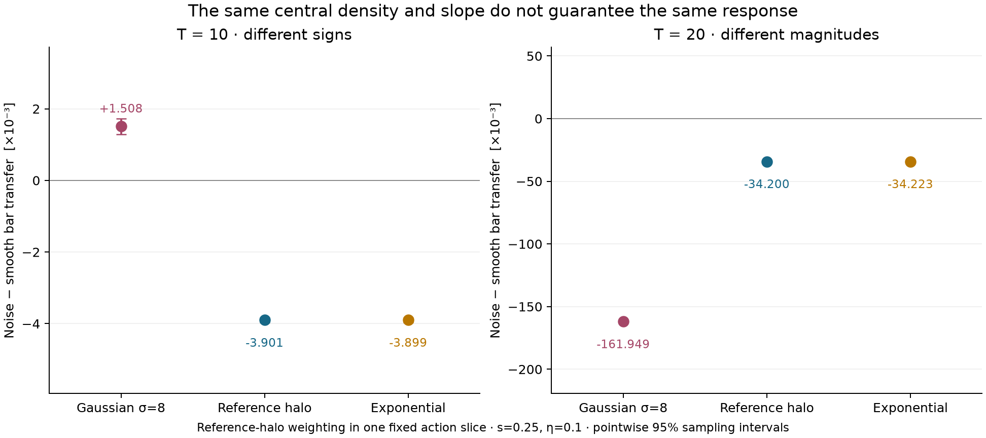
Figure F-POP-01 shows the result of changing only the initial weight. At \(T=10\), diffusion increases the Gaussian's accumulated transfer by \(1.51\times10^{-3}\), but decreases the halo-weighted transfer by \(3.90\times10^{-3}\). The sampling intervals resolve both signs, and the signs survive the specified timestep and window checks. Matching the initial density and slope therefore does not preserve even the direction of the noise-induced change in this example.
At \(T=20\), diffusion decreases the transfer for both populations. The Gaussian response is \(-0.16195\), compared with \(-0.03420\) for the halo, a magnitude ratio of **4.735323**. Suppression thus survives replacing the Gaussian by the reference halo population, but its magnitude is much smaller. The exponential gives \(-0.003899\) and \(-0.034223\) at the two times. Its point differences from the halo are only about 0.050 and 0.068 per cent. These close means do not by themselves establish accuracy at that level; such a claim would require the paired uncertainty and numerical error of the difference.
**Figure F-POP-01.** Change in accumulated bar transfer caused by diffusion, for populations with the same density and slope at the initial resonance. The Gaussian gives the wrong early sign relative to the reference halo weighting and a larger late suppression; the exponential closely follows the reference. Both panels use s = 0.25, η = 0.1 and the cutoff-40 window. The ordinate is the dimensionless response \(\mathcal R[w]\), conditional on one fast-action slice. Error bars are pointwise 95 per cent Student-t intervals from eight independent batches; they do not include numerical sensitivity. The panels show two measured endpoints, with different vertical scales. [Values and numerical controls](https://raw.githubusercontent.com/djova/bar-halo-benchmark/publication-2026-09-24.2/publication/web/results/populations.json).
| Population | T | Response | 95% lower | 95% upper | Numerical/window qualified |
| --- | --- | --- | --- | --- | --- |
| Gaussian σ=8 | 10 | 0.00150764622 | 0.00128939881 | 0.00172589363 | yes |
| Reference halo | 10 | -0.00390067586 | -0.00396285817 | -0.00383849356 | yes |
| Slope-matched exponential | 10 | -0.0038987336 | -0.00396095025 | -0.00383651696 | yes |
| Gaussian σ=8 | 20 | -0.161949145 | -0.162575063 | -0.161323226 | yes |
| Reference halo | 20 | -0.0342002314 | -0.034326595 | -0.0340738678 | yes |
| Slope-matched exponential | 20 | -0.0342234835 | -0.0343499518 | -0.0340970151 | yes |
This result suggests a more precise question than whether the initial curvature is small. Over which actions must the approximation preserve the population gradient? A difference far from the dynamically relevant region need not affect the transfer. Conversely, a modest difference can matter if it changes the balance of large, oppositely signed contributions. We use the response kernel to identify that region and measure this balance.
## The action-dependent response {#kernel}
Because the bar and the noise do not depend on the population, the orbit calculation can be performed before choosing its weight. Define
Response kernel
```math
\begin{aligned}
K_B(x)&=\mathbb E[B_{\rm noise}-B_{\rm smooth}\mid x],\\
\mathcal R[w]&=\int w(x)K_B(x)\,\mathrm dx.
\end{aligned}
```
The expectation averages over initial phase and noise. The kernel measures what the imposed dynamics do to particles starting at \(x\); the weight specifies how much material starts there. Trapping can make an individual trajectory highly nonlinear without spoiling this separation. It requires only that changing the population leave the evolution law unchanged.
Let \(Q_{\rm p}\) be a primitive of \(K_B\). Integration by parts gives
Gradient representation
```math
\mathcal R[w]=[wQ_{\rm p}]_{\rm boundary}
-\int w'(x)Q_{\rm p}(x)\,\mathrm dx.
```
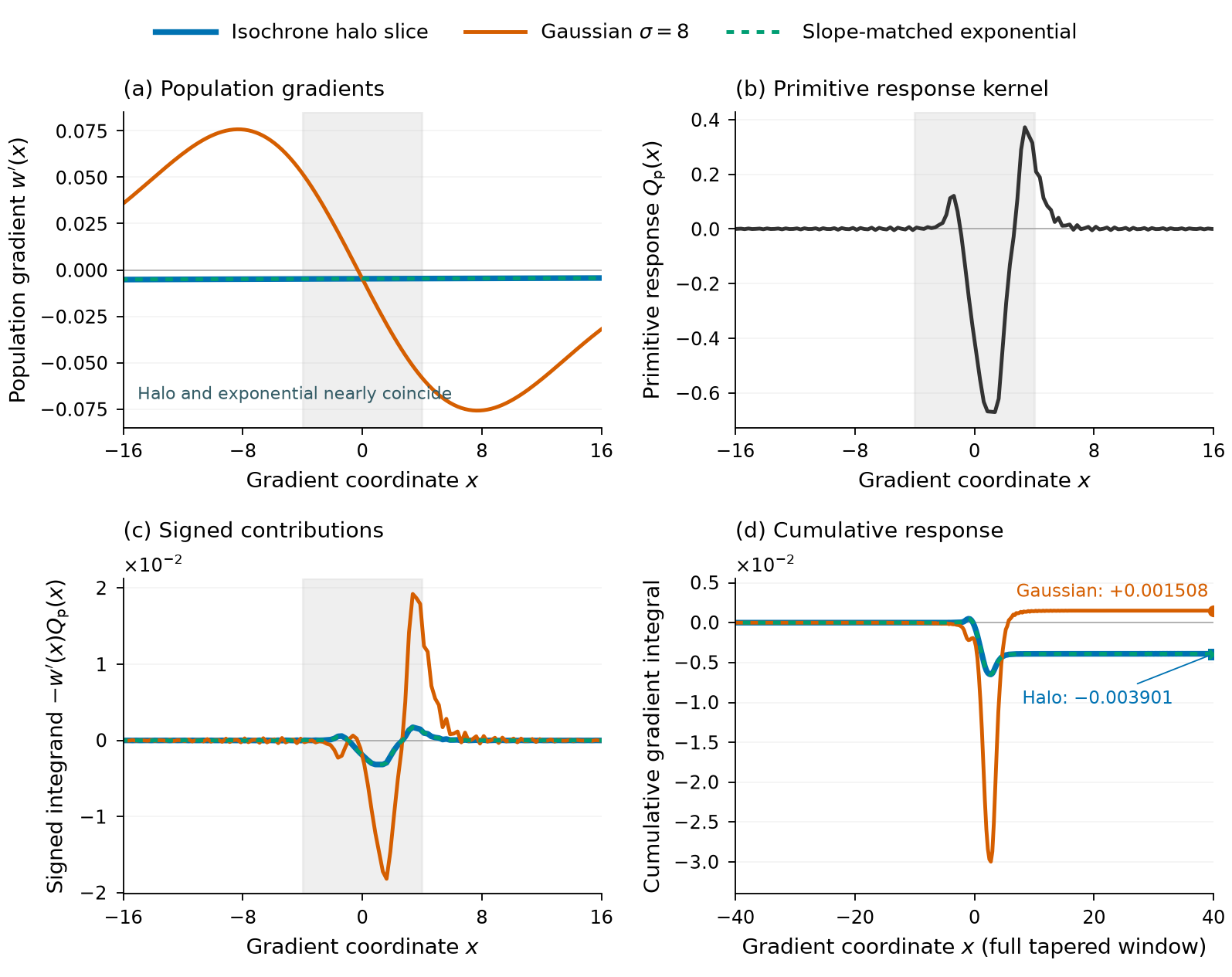
Figure F-GRAD-01 displays the ingredients of this integral. The boundary term vanishes for the compact windows used here. This form shows exactly which population gradients matter: the contribution at each action is \(-w'Q_{\rm p}\). It also explains why agreement at the initial resonance is insufficient. The Gaussian changes the derivative away from that point, where the primitive kernel can still be appreciable.
**Figure F-GRAD-01.** How population gradients weight the recorded response at T = 10, s = 0.25 and η = 0.1. (a) Population gradients; (b) their common primitive kernel; (c) signed contributions to the gradient integral; (d) cumulative response across the complete cutoff-40 window. The grey strip marks \(|x|<4\). Panels (a)–(c) show the central interval \(|x|\leq16\). Products are evaluated on the original fine cells before summation into display cells; multiplying the displayed mean curves is not equivalent. Shaded curve bands are pointwise 95 per cent Student-t intervals from eight batches, without numerical-error expansion. These are terms in the integration-by-parts representation, not separate cohorts of initial orbits. The explanatory curves describe the recorded kernel estimate; the sampling and numerical checks for the endpoint values are supplied with Figure F-POP-01.
For the Gaussian at \(T=10\), integrating the gradient contribution inside and outside \(|x|=4\) gives approximately \(-0.011058\) and \(+0.012565\). Their sum is positive. For the halo, the corresponding contributions are \(-0.004835\) and \(+0.000934\), giving a negative sum. The Gaussian's imposed curvature changes this balance enough to reverse the sign. The exponential, whose gradient remains close to the halo's over the relevant interval, largely preserves it.
This decomposition explains the population dependence of the measured response. It does not by itself separate diffusion-supported friction from changes in resonant capture: that would require additional dynamical diagnostics. Its use here is to calculate several population responses from one set of trajectories and to make the error of a chosen approximation explicit.
## Testing a population approximation {#accuracy}
Suppose \(h\) is the reference weight and \(v\) an approximation. Subtracting their gradient representations gives a signed integral of \(v'-h'\). Taking its absolute value yields
Population-error bound
```math
\left|\mathcal R[v]-\mathcal R[h]\right|
\leq \int |v'(x)-h'(x)|\,|Q_{\rm p}(x)|\,\mathrm dx.
```
This bound is exact for an exact kernel and the stated boundary treatment. It is small when the approximation preserves the gradient where the response is sensitive. Its limitation is equally clear: taking absolute values loses cancellations, so the bound can be larger than the actual error.
In practice, \(Q_{\rm p}\) is estimated from trajectories. We enlarge the gradient integral to account for its sampling uncertainty and measured numerical sensitivity, then add the uncertainty in the approximate response itself. We accept an approximation at the requested accuracy only when this total allowance lies below the target. For the 5 per cent tests, the absolute target is set using a conservative lower estimate of the reference response. A separate sign test asks whether the expanded response interval excludes zero.
The sampling calculation uses eight independent batches and a Student-t envelope with Bonferroni allocation over the specified kernel cells and scalar estimates. Paired timestep differences and factor-two mesh refinements supply numerical-error estimates. These choices produce a reproducible decision rule, but its coverage is approximate: the exact inequality does not turn sampled kernels or refinement differences into rigorous error bounds.
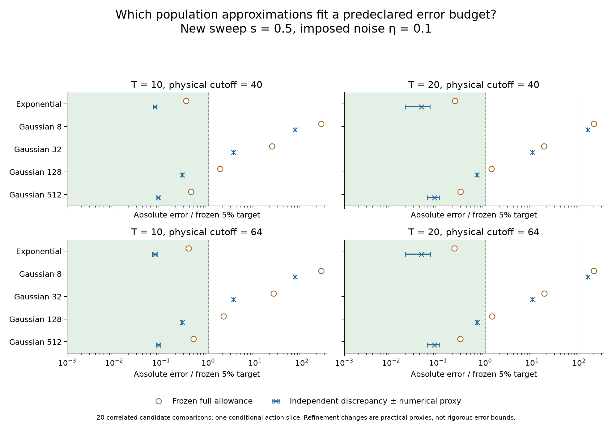
We tested the rule at \(s=0.5\), twice the original sweep rate, keeping \(\eta=0.1\). The new dynamics require a new kernel. The candidate family comprises the exponential and Gaussians with \(\sigma=8,32,128,512\), at both endpoints and both windows. These choices and the decisions were fixed before the independent distribution calculations were examined. Figure F-ACC-01 compares the resulting error allowances with the independent outcomes. Among twenty candidate comparisons, the rule accepted eight: the exponential and Gaussian of width 512 at two times and two windows. All eight meet the specified 5 per cent target in the independent calculation, including its numerical-error estimates. The comparisons share one dynamical condition and one sampled kernel; their count does not represent eight independent physical regimes.
**Figure F-ACC-01.** Performance of the population-error test at s = 0.5 and η = 0.1. Orange circles show the total error allowance divided by the frozen 5 per cent target. Blue crosses show the discrepancy between the approximate response predicted from the kernel and the independently evolved halo response, expanded by the halo's numerical-error estimate and divided by the same target. The latter includes kernel-estimation error, whereas the intrinsic population error compares independently evolved populations. All eight accepted candidates meet the target. Four Gaussian-128 comparisons also meet it but are rejected by the test; eight remaining candidates are independently outside the target. Four halo self-references are excluded from these counts. [Full values](#table-accuracy).
The four conservative rejections illustrate the cost of discarding cancellation. For Gaussian 128 at \(T=10\) in the primary window, the signed population contrast from the mean kernel is approximately \(9.48\times10^{-5}\) in magnitude. The integral of the absolute gradient contributions is \(5.20\times10^{-4}\), already larger than the \(4.38\times10^{-4}\) target before adding kernel uncertainty. More precise kernel sampling does not restore the cancellation discarded by taking absolute values. The test can therefore identify useful approximations while declining some that would in fact be accurate.
### Explore the error calculation {#interactive-decision}
[Interactive decision explorer — requires the canonical site](https://djova.ca/galaxy-bar/paper.html#interactive-decision) · [Static accuracy values — available in this mirror](https://raw.githubusercontent.com/djova/bar-halo-benchmark/publication-2026-09-24.2/publication/web/results/accuracy.json). All recorded outcomes are also tabulated below.
### Complete accuracy values {#table-accuracy}
| ID / population · T · window | Kernel forecast | Independent response | Intrinsic error ± proxy | Forecast − independent halo | Full allowance / 5% target | Advance 5% / independent |
| --- | --- | --- | --- | --- | --- | --- |
| Reference halo · 10 · 40 (reference) | -0.00886738702 | -0.0088400079 | 0 ± 0 | -2.73791146e-05 | 0.000113244174 / 0.000437707142 | Qualified / independently within 5% |
| Slope-matched exponential · 10 · 40 | -0.0088723455 | -0.00884491869 | -4.91078514e-06 ± 7.70468092e-09 | -3.23375997e-05 | 0.000148862064 / 0.000437707142 | Qualified / independently within 5% |
| Gaussian σ=8 · 10 · 40 | -0.0398135751 | -0.0396109614 | -0.0307709535 ± 3.05130755e-05 | -0.0309735672 | 0.113123884 / 0.000437707142 | Not qualified / independently outside 5% |
| Gaussian σ=32 · 10 · 40 | -0.0103457493 | -0.0103050984 | -0.00146509045 ± 2.23114269e-06 | -0.00150574144 | 0.0100394536 / 0.000437707142 | Not qualified / independently outside 5% |
| Gaussian σ=128 · 10 · 40 | -0.00896218156 | -0.0089338922 | -9.38842914e-05 ± 1.47467e-07 | -0.000122173657 | 0.000794600692 / 0.000437707142 | Not qualified / independently within 5% |
| Gaussian σ=512 · 10 · 40 | -0.00887795134 | -0.00885047045 | -1.04625485e-05 ± 1.64425664e-08 | -3.79434334e-05 | 0.000189338267 / 0.000437707142 | Qualified / independently within 5% |
| Reference halo · 10 · 64 (reference) | -0.00886970857 | -0.0088424281 | 0 ± 0 | -2.72804678e-05 | 0.000125126449 / 0.000437229106 | Qualified / independently within 5% |
| Slope-matched exponential · 10 · 64 | -0.00887466249 | -0.00884733137 | -4.90327501e-06 ± 1.07602545e-08 | -3.22343933e-05 | 0.000167582146 / 0.000437229106 | Qualified / independently within 5% |
| Gaussian σ=8 · 10 · 64 | -0.039813574 | -0.0396109618 | -0.0307685337 ± 2.96698035e-05 | -0.0309711459 | 0.112054479 / 0.000437229106 | Not qualified / independently outside 5% |
| Gaussian σ=32 · 10 · 64 | -0.0103469499 | -0.0103061665 | -0.00146373843 ± 2.43893043e-06 | -0.00150452184 | 0.0108583051 / 0.000437229106 | Not qualified / independently outside 5% |
| Gaussian σ=128 · 10 · 64 | -0.00896441884 | -0.00893617755 | -9.37494552e-05 ± 1.95531726e-07 | -0.000121990741 | 0.000929584953 / 0.000437229106 | Not qualified / independently within 5% |
| Gaussian σ=512 · 10 · 64 | -0.00888026334 | -0.00885287494 | -1.04468434e-05 ± 2.24912369e-08 | -3.78352457e-05 | 0.000215716763 / 0.000437229106 | Qualified / independently within 5% |
| Reference halo · 20 · 40 (reference) | -0.0661634001 | -0.0661331971 | 0 ± 0 | -3.02029798e-05 | 0.000546072501 / 0.00328086638 | Qualified / independently within 5% |
| Slope-matched exponential · 20 · 40 | -0.0662762799 | -0.0662460699 | -0.000112872735 ± 3.18237406e-07 | -0.000143082815 | 0.000753037978 / 0.00328086638 | Qualified / independently within 5% |
| Gaussian σ=8 · 20 · 40 | -0.570824503 | -0.570685682 | -0.504552485 ± 0.00092853291 | -0.504691306 | 0.675506654 / 0.00328086638 | Not qualified / independently outside 5% |
| Gaussian σ=32 · 20 · 40 | -0.0991751529 | -0.0991428226 | -0.0330096254 ± 9.04520944e-05 | -0.0330419558 | 0.0593473779 / 0.00328086638 | Not qualified / independently outside 5% |
| Gaussian σ=128 · 20 · 40 | -0.0683290608 | -0.0682987261 | -0.00216552899 ± 6.11217596e-06 | -0.00219586364 | 0.00451776613 / 0.00328086638 | Not qualified / independently within 5% |
| Gaussian σ=512 · 20 · 40 | -0.0664045621 | -0.0663743443 | -0.000241147163 ± 6.80995613e-07 | -0.000271365005 | 0.000988743067 / 0.00328086638 | Qualified / independently within 5% |
| Reference halo · 20 · 64 (reference) | -0.0661736164 | -0.066142906 | 0 ± 0 | -3.07104753e-05 | 0.000519889295 / 0.00328268636 | Qualified / independently within 5% |
| Slope-matched exponential · 20 · 64 | -0.0662864735 | -0.0662557552 | -0.000112849281 ± 3.14117196e-07 | -0.000143567573 | 0.000733737515 / 0.00328268636 | Qualified / independently within 5% |
| Gaussian σ=8 · 20 · 64 | -0.570824507 | -0.570685685 | -0.504542779 ± 0.000927460422 | -0.504681601 | 0.674266443 / 0.00328268636 | Not qualified / independently outside 5% |
| Gaussian σ=32 · 20 · 64 | -0.0991807238 | -0.0991477929 | -0.0330048869 ± 8.97728828e-05 | -0.0330378178 | 0.0601306957 / 0.00328268636 | Not qualified / independently outside 5% |
| Gaussian σ=128 · 20 · 64 | -0.0683388449 | -0.0683079968 | -0.00216509083 ± 6.0403304e-06 | -0.00219593894 | 0.00461589381 / 0.00328268636 | Not qualified / independently within 5% |
| Gaussian σ=512 · 20 · 64 | -0.0664147295 | -0.0663840031 | -0.000241097167 ± 6.7249861e-07 | -0.000271823514 | 0.000977177308 / 0.00328268636 | Qualified / independently within 5% |
[JSON](https://raw.githubusercontent.com/djova/bar-halo-benchmark/publication-2026-09-24.2/publication/web/results/accuracy.json) · [CSV](https://raw.githubusercontent.com/djova/bar-halo-benchmark/publication-2026-09-24.2/publication/web/results/accuracy.csv). Numeric uncertainty is defined in the protocol above; a deterministic proxy is not a sampling confidence interval.
Computing the new kernel required about 5,105 worker CPU-seconds; evaluating the six-profile diagnostic took about 0.8 seconds. The kernel is the expensive step. Once it and the full reference DF are available, directly contracting them is also cheap. The error test is useful for assessing a simplifying population choice, not as a claim that approximating a known DF is always faster than using it.
## Estimating small transfers efficiently {#estimator}
Directly averaging weighted impulses can be inefficient. An individual orbit may gain or lose much more angular momentum than the net transfer of a broad population. The estimate then depends on cancellation between large sampled terms. We reduce that variance by subtracting a control whose integrated expectation is known to vanish.
Let \(F'=w\). From the action budget, removing the coordinate shift and random impulse gives \(y=j+sT-\Xi_T=x+B\). For a fixed noise history, the map from the initial phase plane to \(\psi,y\) preserves area. The time derivative of the integrated primitive displacement can therefore be written as an integral of \(-w(y)\sin\psi\) over that plane. Its angular average vanishes, and the primitive displacement is initially zero. With uniform initial phase and sufficient auxiliary action support, the finite displacement \(F(x+B)-F(x)\) has zero integrated expectation. Consequently,
Finite-displacement estimator
```math
\begin{aligned}
\int w(x)\,\mathbb E[B]\,\mathrm dx
&=-\int\mathbb E\!\left[F(x+B)-F(x)-w(x)B\right]\,\mathrm dx.
\end{aligned}
```
The left-hand side is the generally nonzero transfer. On the right, the first-order term has cancelled *inside the remainder*. For a weight that varies slowly over the displacement, the remainder begins with \(w'B^2/2\); the estimator uses its negative. This replaces a large fluctuating impulse by a smaller quantity controlled by the variation of the weight.
The identity needs more than area preservation alone. The auxiliary initial-action region must extend beyond the physical support by the maximum bar impulse, so that translated trajectories are accounted for even when their starting weights vanish. Those auxiliary samples add no physical mass. The [derivation](https://raw.githubusercontent.com/djova/bar-halo-benchmark/publication-2026-09-24.2/publication/web/methods/CUMULATIVE_IDENTITY.md) specifies the support and symmetry assumptions; action-dependent noise, nonuniform initial phases or a responding halo require a new argument. We apply the identity separately to the noisy and smooth transfers and subtract them.
Variance reduction by subtracting a known contribution is established practice. In cosmological neutrino calculations, [Elbers et al. (2021)](https://arxiv.org/pdf/2010.07321) use a δf construction to sample departures from a reference distribution. Our control instead uses the finite-displacement identity for the accumulated bar impulse. The useful question is how much this particular construction reduces variance for the present target, and where it ceases to help.
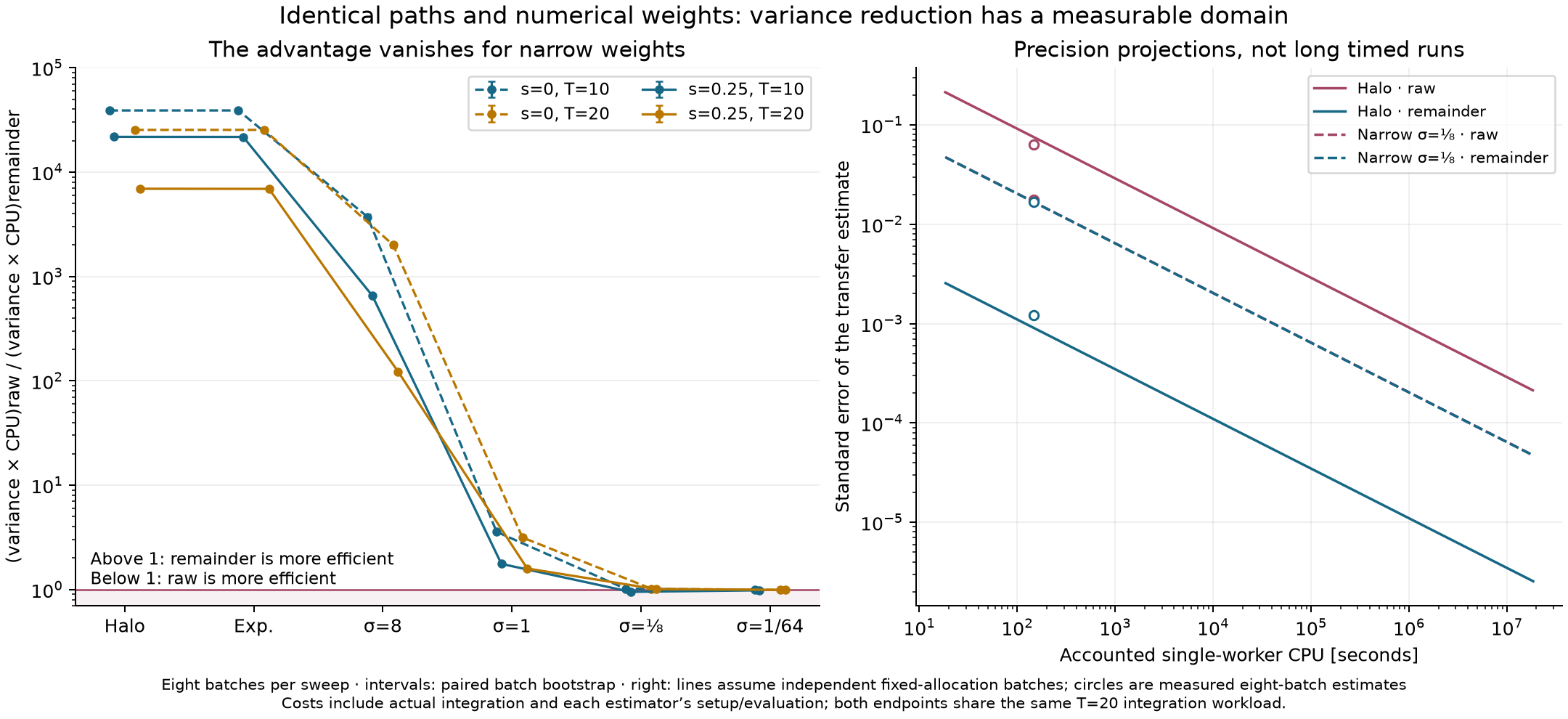
**Figure F-COST-01.** Efficiency of the finite-displacement estimator on matched paths and weights. Left: raw-to-remainder cost-times-variance ratio. Right: precision projected under independent repetition of the measured batch workload, with circles marking the eight-batch estimates. The broad halo population benefits strongly, whereas the narrowest Gaussian does not. Costs include trajectory integration to T = 20, paired timestep refinement, setup and method-specific evaluation; both methods exclude I/O and common covariance assembly. T = 10 receives the same full-workload cost. Intervals are whole-batch bootstrap intervals. Conditional and between-batch variance estimates are reported separately in the [complete records](#table-cost).
Figure F-COST-01 shows the measured efficiency across broad and narrow weights. For the halo weight at \(s=0.25\), \(T=20\), the raw and remainder calculations cost about 18.40 and 18.56 CPU-seconds per batch. Their conditional cost-times-variance ratio is approximately 6,928; using the noisier variance between the eight batches gives about 2,749. The gain comes from lower variance, not faster orbit integration. For a Gaussian of width \(1/64\), the ratio is about 0.993 and the advantage disappears, as expected when the weight changes sharply over an impulse displacement. One of the 24 pointwise paired method-comparison intervals excludes zero; it remains in the record and is not, by itself, evidence of bias after multiple comparisons.
[Interactive estimator comparison — requires the canonical site](https://djova.ca/galaxy-bar/paper.html#estimator) · [Static estimator values — available in this mirror](https://raw.githubusercontent.com/djova/bar-halo-benchmark/publication-2026-09-24.2/publication/web/results/cost.json). All recorded outcomes are also tabulated below.
### Complete estimator-cost values {#table-cost}
| Population · s · T | Raw / remainder CPU s | Cost×variance ratio | Bootstrap interval | Between-batch ratio | Raw−remainder 95% interval |
| --- | --- | --- | --- | --- | --- |
| halo · 0.0 · 10 | 18.2927416 / 18.4636202 | 38988.5558 | [38008.699, 40043.7838] | 89013.143 | [-0.0469247543, 0.111264275] |
| exponential · 0.0 · 10 | 18.2873912 / 18.4509676 | 39002.9004 | [38024.4573, 40062.5082] | 89093.6618 | [-0.0469219707, 0.111260408] |
| gaussian8 · 0.0 · 10 | 18.2879427 / 18.4467792 | 3730.44102 | [3579.87624, 3919.33533] | 6777.02582 | [-0.0370077712, 0.102973788] |
| stress1 · 0.0 · 10 | 18.2888599 / 18.4464164 | 3.57293977 | [3.46038643, 3.69321681] | 2.10966059 | [0.00189734593, 0.0705498717] |
| stress0.125 · 0.0 · 10 | 18.2890393 / 18.4529955 | 1.0167378 | [0.997359472, 1.03637194] | 0.689486757 | [-0.0025506543, 0.0206194091] |
| stress0.015625 · 0.0 · 10 | 18.2880118 / 18.4515892 | 0.992355072 | [0.982503353, 0.998662704] | 1.17587075 | [-0.000333731476, 0.00301891144] |
| halo · 0.0 · 20 | 18.2927416 / 18.4636202 | 25391.9454 | [24624.54, 26166.9585] | 13958.0278 | [-0.0387549753, 0.150559704] |
| exponential · 0.0 · 20 | 18.2873912 / 18.4509676 | 25401.5441 | [24632.1593, 26179.7586] | 13964.1292 | [-0.0387520904, 0.150550573] |
| gaussian8 · 0.0 · 20 | 18.2879427 / 18.4467792 | 1999.34617 | [1891.74532, 2113.27781] | 1984.36574 | [-0.0302260419, 0.137654808] |
| stress1 · 0.0 · 20 | 18.2888599 / 18.4464164 | 3.15315647 | [3.08115964, 3.22569516] | 2.33288971 | [-0.0199932485, 0.0833105724] |
| stress0.125 · 0.0 · 20 | 18.2890393 / 18.4529955 | 1.0179098 | [0.990506414, 1.04162801] | 1.01849023 | [-0.00680509509, 0.0175994924] |
| stress0.015625 · 0.0 · 20 | 18.2880118 / 18.4515892 | 0.992678781 | [0.982394718, 0.999541036] | 1.06109263 | [-0.00124153863, 0.0023117685] |
| halo · 0.25 · 10 | 18.3951548 / 18.5555606 | 21774.1766 | [21232.2166, 22388.9995] | 15771.4777 | [-0.154478939, 0.0515187704] |
| exponential · 0.25 · 10 | 18.3893467 / 18.5494944 | 21737.6501 | [21193.2822, 22346.4601] | 15751.2286 | [-0.154477821, 0.0515151541] |
| gaussian8 · 0.25 · 10 | 18.3900161 / 18.5535038 | 655.056603 | [642.440071, 668.687611] | 595.86026 | [-0.145108703, 0.0453767745] |
| stress1 · 0.25 · 10 | 18.3910858 / 18.5584824 | 1.76012886 | [1.72686248, 1.7918993] | 1.51851776 | [-0.0430420305, 0.0217359335] |
| stress0.125 · 0.25 · 10 | 18.3917059 / 18.5551953 | 0.950669603 | [0.929711113, 0.970806296] | 1.21402495 | [-0.00742977169, 0.00469680938] |
| stress0.015625 · 0.25 · 10 | 18.3913661 / 18.5558685 | 0.982318106 | [0.976786364, 0.987149269] | 1.00221341 | [-0.00100054773, 0.000636462618] |
| halo · 0.25 · 20 | 18.3951548 / 18.5555606 | 6928.35383 | [6734.74079, 7229.0683] | 2749.39907 | [-0.200904278, 0.0958018925] |
| exponential · 0.25 · 20 | 18.3893467 / 18.5494944 | 6909.883 | [6719.27032, 7205.83238] | 2741.03489 | [-0.200907308, 0.0957963382] |
| gaussian8 · 0.25 · 20 | 18.3900161 / 18.5535038 | 122.402097 | [118.569864, 126.059907] | 48.8071359 | [-0.193000966, 0.0795659508] |
| stress1 · 0.25 · 20 | 18.3910858 / 18.5584824 | 1.59023169 | [1.57376204, 1.60533648] | 1.23894207 | [-0.0522395946, 0.0108568746] |
| stress0.125 · 0.25 · 20 | 18.3917059 / 18.5551953 | 1.00717161 | [1.00078163, 1.01310713] | 1.08977343 | [-0.00642130534, 0.00555408516] |
| stress0.015625 · 0.25 · 20 | 18.3913661 / 18.5558685 | 0.992683075 | [0.990994634, 0.994227314] | 1.04131574 | [-0.0010128956, 0.000780686105] |
[JSON](https://raw.githubusercontent.com/djova/bar-halo-benchmark/publication-2026-09-24.2/publication/web/results/cost.json) · [CSV](https://raw.githubusercontent.com/djova/bar-halo-benchmark/publication-2026-09-24.2/publication/web/results/cost.csv). All 24 endpoints retain their paired consistency assessments.
## Discussion and conclusions {#limitations}
The population choice can alter a finite-time noise response even when central density and slope are matched. In our example, the Gaussian gives the opposite early sign from the reference halo slice and a late suppression about 4.7 times larger. The exponential succeeds much better because its gradient follows the reference over the actions that contribute to the response. The relevant matching condition is therefore distributed over that interval, rather than confined to the initial resonance.
The response kernel makes this statement quantitative. It identifies how changes in the population gradient affect the transfer and provides an error test that can be evaluated before a new population is evolved. At the second sweep rate, the accepted approximations satisfy the independent numerical comparison. The conservative rejections show that this usefulness comes with a limitation: an absolute bound can discard cancellation essential to the final answer. A failure to accept an approximation need not mean that the approximation is inaccurate.
These conclusions concern a fixed external evolution. The halo DF enters as an initial weight on one pair of fast actions; it does not generate a responding potential. In a self-consistent system, redistribution of particles can alter the forces and resonance locations. The connection between DF structure and dynamical friction in such systems is discussed, for example, by [Dattathri et al. (2026)](https://arxiv.org/abs/2511.11804v2), but their collective core dynamics are absent from this model. The present calculation neither measures a full-halo torque nor provides a universal correction for one.
The constant coefficients, additive diffusion, finite population window and abrupt bar turn-on further define the scope of the result. A different history or noise law requires a new kernel. Our attempted transfer to prescribed-field three-dimensional orbits remains statistically unresolved; even successful agreement there would leave collective halo response untested. The noise coefficient has not been calibrated to dark-matter scattering. **These experiments do not test CDM against SIDM.**
The practical result is a way to assess a population substitution in a controlled resonance calculation: compare its gradient with the reference over the region weighted by the kernel, retain cancellation when computing the response, and include kernel uncertainty when assessing the error. The finite-displacement estimator makes that assessment affordable for broad populations. Its extension to a broader range of resonances and noise histories can be tested independently of the population example presented here.
## Supporting evidence and earlier studies {#models}
The main argument above is self-contained. This section connects it to the machine-readable records and to earlier investigations without treating their different physical models as interchangeable.
| Model ID | What evolves | What this establishes | Clock / methods |
| --- | --- | --- | --- |
| GAL-LIVE — Self-gravitating galaxy and its fixed-field controls | Stellar and halo particles; live components alter gravity. Named frozen/static controls remove specified response. | Behavior and numerical sensitivity of the specified galaxy models; No SIDM comparison; no converged universal bar-strength prediction | Gyr; kpc; solar masses · [methods — historical website-only](https://djova.ca/galaxy-bar/methodology.html) |
| CART-EXT — Prescribed-field Cartesian orbits | Test particles in an external analytical field, imposed bar and disturbances; cloud does not react collectively | Particle response to those specified external fields; Not live-halo validation | Analytical-potential model time/action · [methods — historical website-only](https://djova.ca/galaxy-bar/response-methods.html) |
| RES-POS — Reduced noisy resonance, positive population | Slow action and resonant angle; constant additive action diffusion; fixed fast-action slice | Population response and numerical accuracy within this local operator; Not full-halo torque, SIDM or general confidence coverage | Dimensionless T, x and impulse B · [methods](https://raw.githubusercontent.com/djova/bar-halo-benchmark/publication-2026-09-24.2/publication/web/paper.md#model) |
| RES-SIGNED — Earlier signed perturbation with reservoirs | Signed deviation with its own reservoir/boundary conditions | Verification and response of that separate setup; Not interchangeable with positive-population results | Its documented reduced-model units · [methods — historical website-only](https://djova.ca/galaxy-bar/noise-methods.html) |
| SYNTH — Synthetic controls | Known stochastic laws or analytical limiting processes | Verification of estimators, coordinates or numerical algorithms; Not a new astrophysical measurement | Control-specific units · [methods — historical website-only](https://djova.ca/galaxy-bar/response-validation.html) |
POP-01 · At s=0.25, Gaussian and reference-halo weighting in the tested slice have opposite T=10 responses; their T=20 suppression magnitudes differ by 4.735323.
PA-ACC-01 · Eight advance 5% qualifications are supported by independent numerical comparison at one new sweep rate, s=0.5.
PA-ACC-02 · Four Gaussian-128 comparisons meet 5% in the independent assessment but are not qualified by the conservative absolute-gradient allowance.
EST-01 · The matched estimator has a large conditional cost-times-variance advantage for broad halo weights; the advantage disappears for the narrowest stress population.
**LIM-01.** One isochrone fast-action slice and finite windows/times; no total halo torque or universal 4.7 correction.
**LIM-02.** Imposed bar and population-independent additive noise; no collective halo response or calibrated SIDM operator.
**LIM-03.** Approximate sampling coverage and numerical-refinement proxies; no rigorous operational 5% guarantee.
**LIM-04.** Eight qualified comparisons share one new dynamical condition and correlated kernel; no eight independent physical regimes.
**LIM-05.** Prescribed-field 3D transfer remains unresolved; even successful transfer would not validate a live halo.
**LIM-06.** Cost-times-variance ratios project precision under a fixed workflow; no measured 6900-fold faster simulation.
**LIM-07.** Specific estimator priority and astrophysical generalization remain open; not externally reviewed.
**LIM-08.** Software reproduction and deployment checks do not independently confirm physics.
The earlier 24 population forecasts passed their original criterion, max(0.0002, 5% of forecast). A later assessment combining numerical-error estimates leaves two early Gaussian-12 window comparisons marginal. Their original outcomes remain unchanged in the [historical assessment](https://raw.githubusercontent.com/djova/bar-halo-benchmark/publication-2026-09-24.2/publication/web/diagnostics/population-accuracy/joint-error-assessment.json). The prescribed-field study also retains two separate corrections: the smooth response replicated under new phases at the same actions and forcing, and constant diffusion with restoring drift can fail a flat finite-lag variance screen. Neither correction is a result of the present population comparison. [Earlier response study — historical website-only](https://djova.ca/galaxy-bar/response.html).
## Data, code and correspondence {#reproduction}
The [public benchmark](https://github.com/djova/bar-halo-benchmark) contains inputs, numerical methods and reproduction commands. The [reproduction map](https://raw.githubusercontent.com/djova/bar-halo-benchmark/publication-2026-09-24.2/publication/web/reproduce.md) distinguishes checking supplied values from rerunning the evolution and states the coverage of each released study. The archived project receipt documents exact reproduction of 162 saved arrays; that is software reproducibility, not additional physical sampling or external scientific review.
REP-01 · The project receipt documents exact reproduction of 162 saved arrays from the released numerical source. This publication campaign does not claim a new rerun.
Questions and corrections can be submitted through the [public issue tracker](https://github.com/djova/bar-halo-benchmark/issues), using an equation, figure or claim identifier and the release version. Analysis, software and exposition were developed with AI assistance. The human project maintainer is djova; no institutional affiliation or outside endorsement is asserted.
**Release 2026-09-24.2:** rewrites the physical argument, derives the model and scales, documents the initial forcing and tabulated DF, and separates the manuscript from the website’s supporting records. An added figure shows the existing gradient-kernel data; no trajectories or scientific outcomes changed. The [editorial correction — historical website-only](https://djova.ca/galaxy-bar/communication.html#editorial-20260924) records the diagnosis and revised skill. Earlier releases remain unchanged. [Archive — historical website-only](https://djova.ca/galaxy-bar/archive.html) · [manifest](https://raw.githubusercontent.com/djova/bar-halo-benchmark/publication-2026-09-24.2/publication/web/manifest.json) · [reuse conditions](https://raw.githubusercontent.com/djova/bar-halo-benchmark/publication-2026-09-24.2/publication/web/reproduce.md#licenses).
## References and reading record {#references}
Primary links appear beside the associated statements. [Original scholarly sources — historical website-only](https://djova.ca/galaxy-bar/diagnostics/population-accuracy/SOURCES.md) and [publication review sources](https://raw.githubusercontent.com/djova/bar-halo-benchmark/publication-2026-09-24.2/publication/web/publication-sources.md) identify the inspected material and its limits. Accessibility follows the [W3C complex-image guidance](https://www.w3.org/WAI/tutorials/images/complex/) through readable captions and complete values. Registry design follows [FAIR principles](https://www.gofair.foundation/fair-principles); no formal certification is claimed.