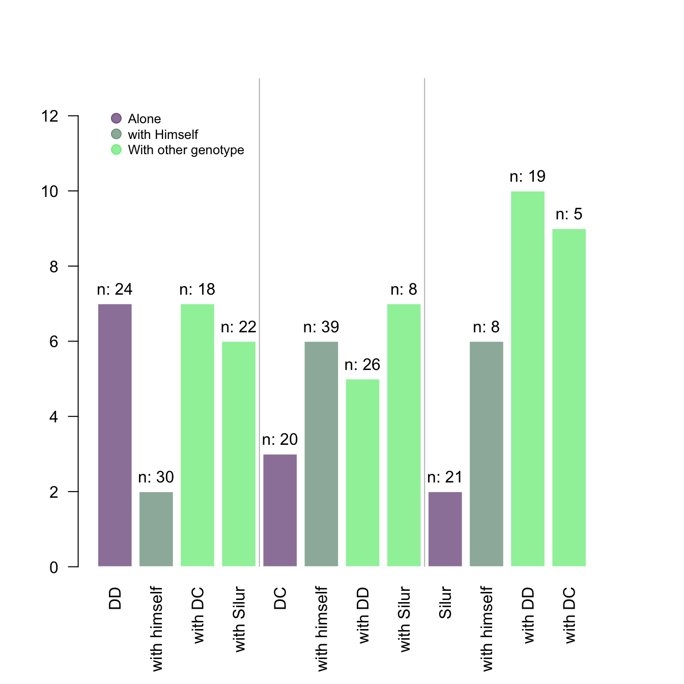
This chart illustrates many tips you can apply to a base R barplot:
- Add abline with
abline() - Change axis labels orientation with
las - Add text with
text() - Add a legend with
legend()

# Data
data <- data.frame(
  name = c("DD","with himself","with DC","with Silur" ,"DC","with himself","with DD","with Silur" ,"Silur","with himself","with DD","with DC" ),
  average = sample(seq(1,10) , 12 , replace=T),
  number = sample(seq(4,39) , 12 , replace=T)
)

# Increase bottom margin
par(mar=c(6,4,4,4))


# Basic Barplot
my_bar <- barplot(data$average , border=F , names.arg=data$name ,
                  las=2 ,
                  col=c(rgb(0.3,0.1,0.4,0.6) , rgb(0.3,0.5,0.4,0.6) , rgb(0.3,0.9,0.4,0.6) ,  rgb(0.3,0.9,0.4,0.6)) ,
                  ylim=c(0,13) ,
                  main="" )

# Add abline
abline(v=c(4.9 , 9.7) , col="grey")

# Add the text
text(my_bar, data$average+0.4 , paste("n: ", data$number, sep="") ,cex=1)

#Legende
legend("topleft", legend = c("Alone","with Himself","With other genotype" ) ,
     col = c(rgb(0.3,0.1,0.4,0.6) , rgb(0.3,0.5,0.4,0.6) , rgb(0.3,0.9,0.4,0.6) ,  rgb(0.3,0.9,0.4,0.6)) ,
     bty = "n", pch=20 , pt.cex = 2, cex = 0.8, horiz = FALSE, inset = c(0.05, 0.05))


