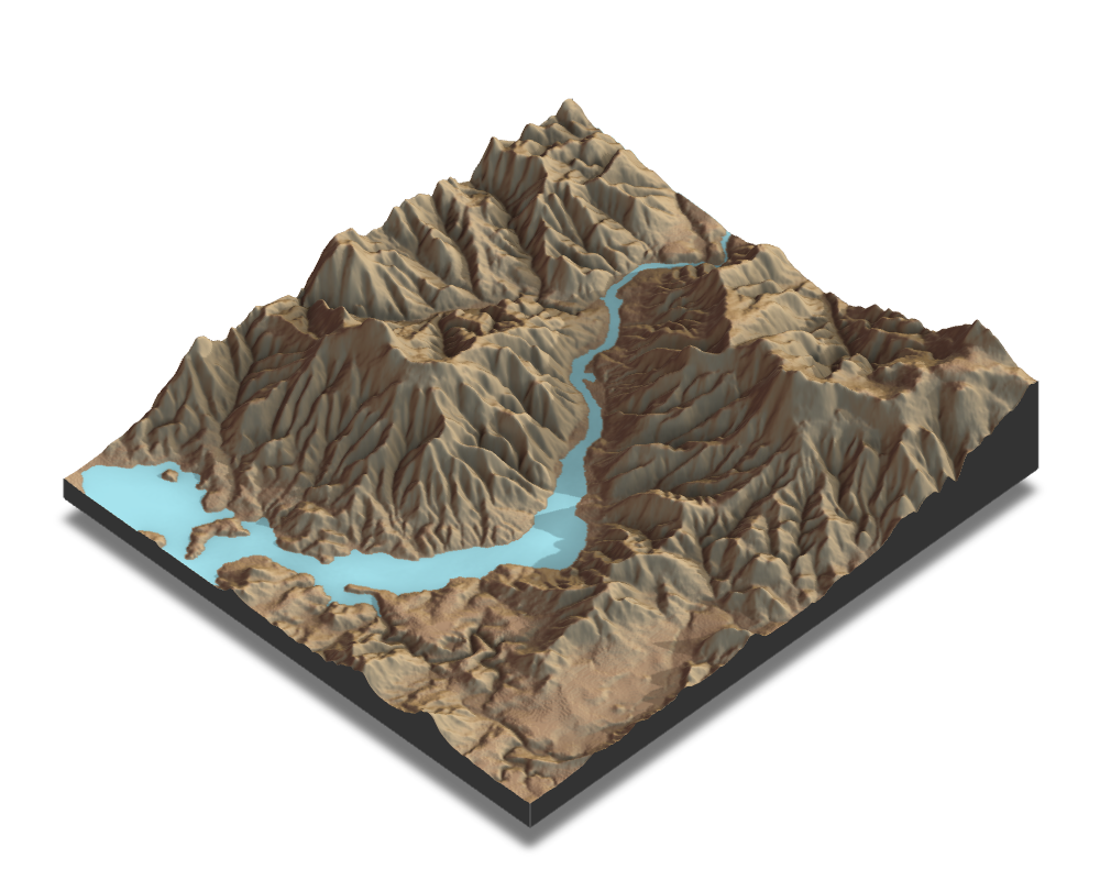
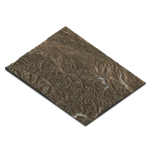
Beautiful shaded maps with rayshader


The rayshader package in R is a highly versatile tool designed to create stunningly detailed shaded maps and 3D visualizations. This comprehensive guide aims to provide an in-depth explanation of how to effectively use the rayshader package, covering its key features and functionalities.

Additionally, it showcases a curated collection of graph examples that highlight the package’s capabilities and potential applications.

Documentation

{rayshader}

Quick start


The rayshader package in R allows us to create beautiful, 2D and 3D shaded maps.

rayshader offers a robust suite of functions for generating beautifully shaded maps in R, allowing for the creation of detailed 3D visualizations. The package includes tools for rendering 3D surfaces, adding textures, and incorporating lighting effects.

Users can control z-scale, shadow depth, and water layers to enhance realism. Additionally, rayshader supports external spatial data integration, enabling complex overlays and customizations.

✍️ author → Tyler Morgan-Wall

📘 documentationgithub

⭐️ more than 1000 stars on github

rayshader example

Installation


To get started with rayshader, you can install it directly from CRAN using the install.packages function:

install.packages("rayshader")

Data format


The rayshader package makes it easy quite easy to create shaded maps but requires the data to be in a specific format.

The data should be a matrix of elevation values. If you’re not used to it, think of matrix as a table where each cell contains a value, like in a dataframe.

You can use the raster package to convert raster data to a matrix.

Example:

library(rayshader)
library(terra)

# Load a raster file
loadzip = tempfile()
download.file("https://tylermw.com/data/dem_01.tif.zip", loadzip)
localtif = raster::raster(unzip(loadzip, "dem_01.tif"))
unlink(loadzip)

# Convert the raster to a matrix
elevation_matrix = raster_to_matrix(localtif)

Once we have the data in the right format, we can start creating shaded maps in just a few lines of code.

Key features


→ Simple 2d maps

rayshader allows you to create simple 2D maps.

Example:

elevation_matrix %>%
  sphere_shade(texture = "desert") %>%
  plot_map()


→ Add water

You can add water to your maps using the detect_water() and add_water() functions.

Example:

elevation_matrix %>%
  sphere_shade(texture = "desert") %>%
  add_water(detect_water(elevation_matrix), color = "desert") %>%
  plot_map()


→ Change the shading and sun position

You can change the shading and sun position using the add_shadow(), ray_shade(), and ambient_shade() functions.

Example:

elevation_matrix %>%
  sphere_shade(texture = "desert") %>%
  add_water(detect_water(elevation_matrix), color = "desert") %>%
  add_shadow(ray_shade(elevation_matrix), 0.5) %>%
  add_shadow(ambient_shade(elevation_matrix), 0) %>%
  plot_map()


→ 3D maps

Using the same data as before, you can create 3D maps with the plot_3d() function. This will enhance the visual aspect of your maps and give them a more realistic look.

Example:

elevation_matrix %>%
  sphere_shade(texture = "desert") %>%
  add_water(detect_water(elevation_matrix), color = "desert") %>%
  add_shadow(ray_shade(elevation_matrix, zscale = 3), 0.5) %>%
  add_shadow(ambient_shade(elevation_matrix), 0) %>%
  plot_3d(elevation_matrix, zscale = 10, fov = 0, theta = 135, zoom = 0.75, phi = 45, windowsize = c(1000, 800))
render_snapshot()

rayshader example


❤️ 10 best R tricks ❤️

👋 After crafting hundreds of R charts over 12 years, I've distilled my top 10 tips and tricks. Receive them via email! One insight per day for the next 10 days! 🔥