Libraries

The rayshader package makes it simple to create shaded 2D relief maps.

Since the package is on CRAN, you can install it with install.packages("rayshader").

We also load the raster package to access data to work with.

# install.packages("rayshader")
library(rayshader)
library(raster)

Data format

The rayshader package requires input data in elevation matrix format. This special matrix has each cell containing the elevation value of the corresponding map point.

Here’s how to obtain the elevation matrix from a raster file using the raster package.

# Define a region for the SRTM data (example: Swiss Alps)
extent_alps <- extent(7.0, 9.0, 46.0, 47.5)

# Download SRTM data
srtm_alps <- getData("SRTM", lon = 8.0, lat = 46.75)

# Crop the SRTM data to the defined extent
srtm_alps_cropped <- crop(srtm_alps, extent_alps)

# Convert the raster data to matrix
elevation_matrix <- raster_to_matrix(srtm_alps_cropped)

Basic 3D map

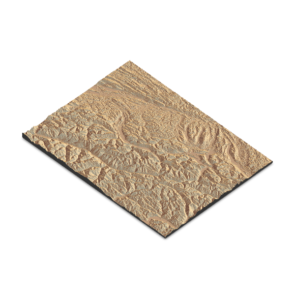
To create a basic 3D map with rayshader using the sphere_shade() and plot_3d() functions, follow these steps:

Load your elevation data.
Generate a shaded texture using sphere_shade().
Render the 3D map using plot_3d().

When you render it, a 3D window will open where you can interact with the map.

elevation_matrix %>%
  sphere_shade(texture="desert", sunangle = 45) %>%
  plot_3d(elevation_matrix, zscale = 50)

render_snapshot('img/graph/411-map-3d-with-rayshader-1.png')

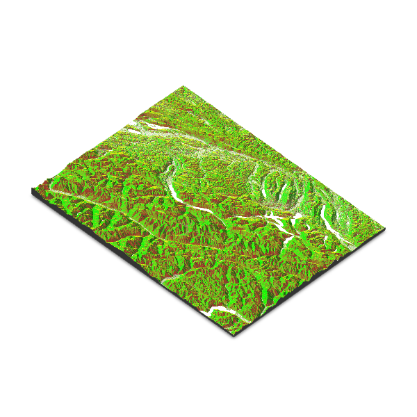
Change texture

rayshader includes a specialized function to create textures: create_texture(). This function accepts 5 colors as input and generates a texture suitable for use in the sphere_shade() function.

texture <- create_texture("darkgreen", "green", "yellow", "brown", "white")
elevation_matrix %>%
  sphere_shade(texture=texture, sunangle = 45) %>%
  plot_3d(elevation_matrix, zscale = 50)
render_snapshot('img/graph/411-map-3d-with-rayshader-2.png')

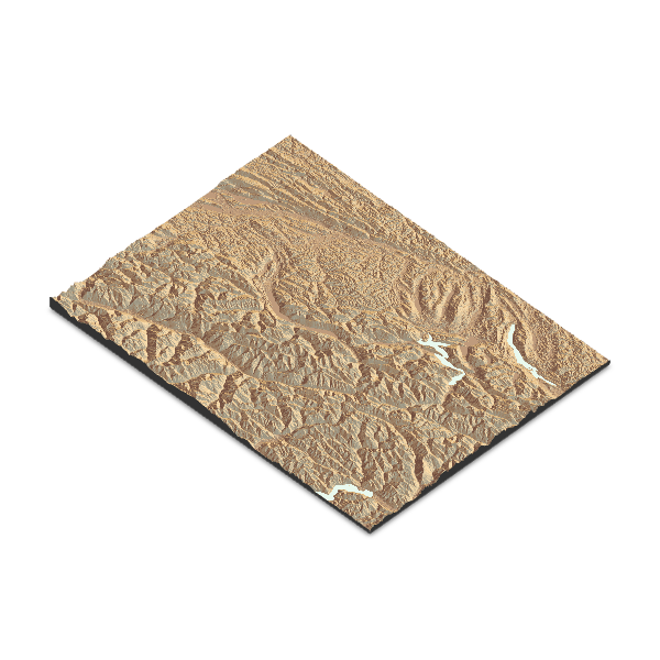
Add water

To add water, you first need to detect the water in the elevation matrix using the detect_water() function.

After that, you can use the add_water() function to integrate the water into the map.

elevation_matrix %>%
  sphere_shade(texture="desert", sunangle = 45) %>%
  add_water(detect_water(elevation_matrix)) %>%
  plot_3d(elevation_matrix, zscale = 50)
render_snapshot('img/graph/411-map-3d-with-rayshader-3.png')

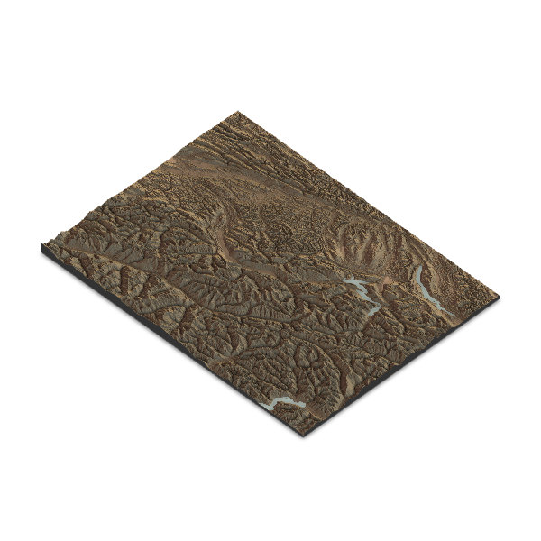
Change shade properties

The add_shadow() function can be used to add a shadow to the map. The ray_shade() function creates a shadow based on the sun angle, while the ambient_shade() function creates a shadow based on the ambient light.

elevation_matrix %>%
  sphere_shade(texture="desert", sunangle = 45) %>%
  add_water(detect_water(elevation_matrix)) %>%
  add_shadow(ray_shade(elevation_matrix), 0.5) %>% # this line adds a shadow
  add_shadow(ambient_shade(elevation_matrix), 0) %>% # this line adds an ambient shadow
  plot_3d(elevation_matrix, zscale = 50)
render_snapshot('img/graph/411-map-3d-with-rayshader-4.png')

3d maps with rayshader