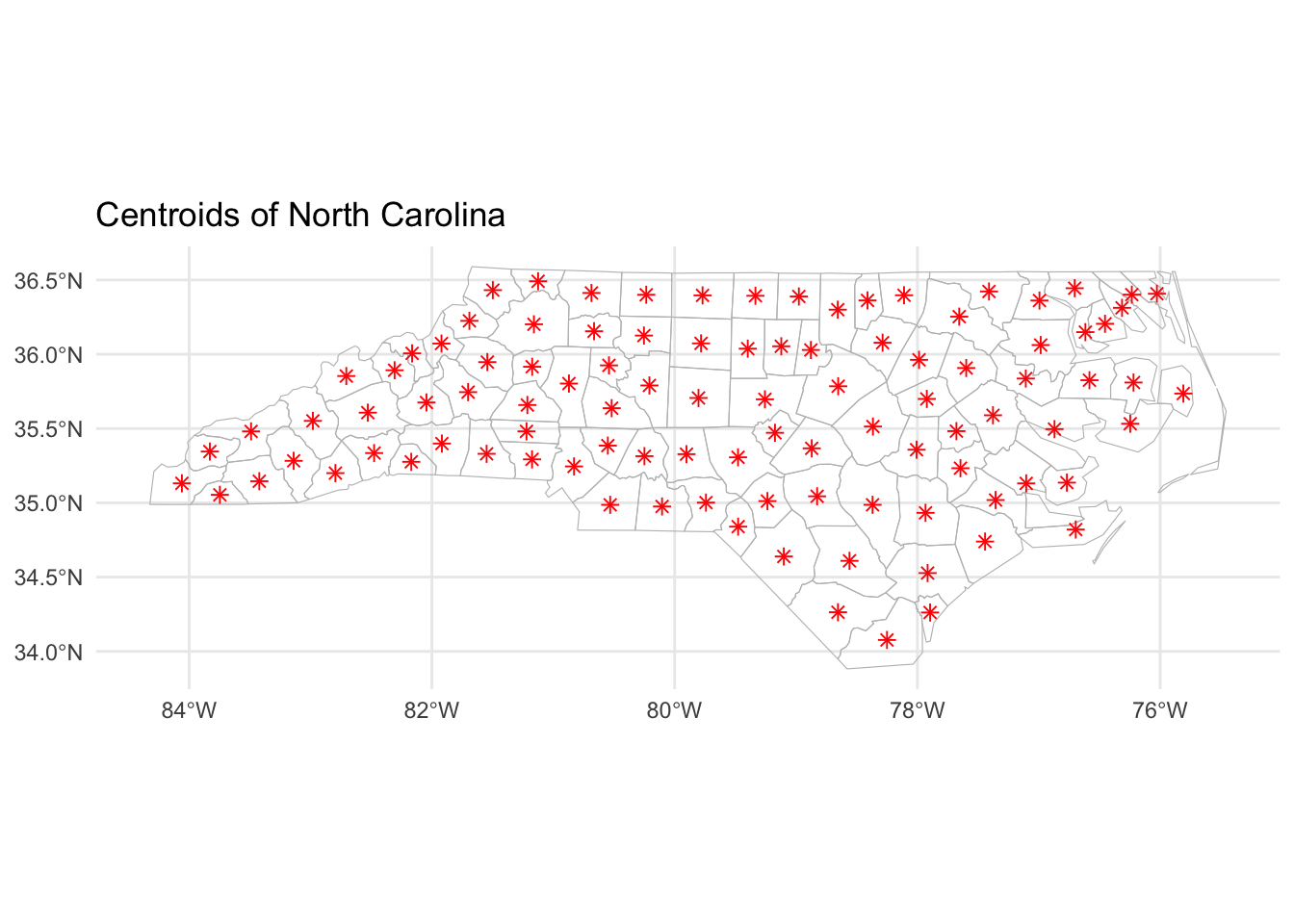
Plot and manipulate geographic features with sf


The sf package in R specializes in geospatial visualization, offering streamlined access to geographic features like points, lines, and polygons, and more generally to create maps.

Documentation

{sf}

Quick start


In just a few lines of code, you can create stunning visualizations with the sf package in R. What’s more, sf lets you create maps from almost any data format, such as shapefiles or geojson. You can learn more about geographical data in the map section.

This package offers a large variety of functions to manipulate and visualize geographic data. The main steps usually are:

  • create a geospatial object with st_read() or read_sf()

  • filter, transform, and manipulate the object for your needs

  • plot the object with plot() or with ggplot2

✍️ author → Edzer Pebesma

📘 documentationgithub

⭐️ more than 1000 stars on github

Installation


To get started with sf, you can install it directly from CRAN using the install.packages function:

install.packages("sf")

Basic usage


The sf package is shipped with the nc dataset, which contains the boundaries of North Carolina.

Here’s a basic example of how to plot the first feature of the nc dataset:

library(sf)
nc <- st_read(system.file("shape/nc.shp", package="sf"), quiet = TRUE)
plot(st_geometry(nc), col = "lightblue", border = "black", lwd = 1.2, main = "North Carolina")

Key features


→ Choropleth Maps

The sf package allows you to create choropleth maps with ease.

Simply use the geom_sf() function with ggplot2 to create a choropleth map of your geographic data.

You can customize the map by specifying the fill aesthetic and the color palette using the scale_fill_viridis_c() function

Example:

library(sf)
library(ggplot2)

# Read the shapefile
nc = st_read(system.file("shape/nc.shp", package="sf"), quiet = TRUE)

# Create the plot using ggplot2
ggplot() +
  geom_sf(data = nc, aes(fill = AREA)) +
  scale_fill_viridis_c() +
  ggtitle('Choropleth Map of North Carolina') +
  theme_minimal()


→ Graticules

Graticules are lines of latitude and longitude that help you orient yourself on a map. You can add graticules to your map using the plot() function.

Example:

library(maps)
library(sf)
library(ggplot2)
library(patchwork)

# create a map of the USA
usa = st_as_sf(map('usa', plot = FALSE, fill = TRUE))
laea = st_crs("+proj=laea +lat_0=30 +lon_0=-95") # Lambert equal area projection
usa2 <- st_transform(usa, laea)

# create ggplot objects with graticules
p1 = ggplot(data = usa) + 
  geom_sf() + 
  theme_minimal()

p2 = ggplot(data = usa2) + 
  geom_sf() + 
  theme_minimal()

# combine plots with patchwork
p1 + p2


→ Compute and plot centroids

You can compute and plot the centroids of your geographic features using the st_centroid() function.

Caution: Centroids serve merely as an approximation of a polygon’s “center” and may not always provide meaningful or accurate insights.

Example:

library(sf)
library(ggplot2)

# Read the shapefile
nc = st_read(system.file("shape/nc.shp", package="sf"), quiet = TRUE)
ncg = st_geometry(nc)
cntrd = st_centroid(ncg)

# Create the plot using ggplot2
ggplot() +
  geom_sf(data = ncg, fill = NA, color = 'grey') +
  geom_sf(data = cntrd, color = 'red', shape = 8, size = 2) +
  ggtitle('Centroids of North Carolina') +
  theme_minimal()


→ What’s more?

While sf is not a data visualization package per se, it provides extensive functionalities for handling and visualizing geographic data. This includes:

  • Creating a geospatial object using st_read() or read_sf() from virtually any file format.
  • Filtering, transforming, and manipulating the geospatial object to suit your specific requirements.
  • Enhancing your visualizations by integrating with other packages, such as ggplot2.

Explore the capabilities of sf below!


❤️ 10 best R tricks ❤️

👋 After crafting hundreds of R charts over 12 years, I've distilled my top 10 tips and tricks. Receive them via email! One insight per day for the next 10 days! 🔥