2.7. Novelty and Outlier Detection
Many applications require being able to decide whether a new observation belongs to the same distribution as exiting observations (it is an inlier), or should be considered as different (it is an outlier). Often, this ability is used to clean real data sets. Two important distinction must be made:
| novelty detection: | |
|---|---|
| The training data is not polluted by outliers, and we are interested in detecting anomalies in new observations. | |
| outlier detection: | |
| The training data contains outliers, and we need to fit the central mode of the training data, ignoring the deviant observations. | |
The scikit-learn project provides a set of machine learning tools that can be used both for novelty or outliers detection. This strategy is implemented with objects learning in an unsupervised way from the data:
estimor.fit(X_train)
new observations can then be sorted as inliers or outliers with a predict method:
estimator.predict(X_test)
Inliers are labeled 0, while outliers are labeled 1.
2.7.1. Novelty Detection
Consider a data set of  observations from the same
distribution described by
  features. Consider now that we
add one more observation to that data set. Is the new observation so
different from the others that we can doubt it is regular? (i.e. does
it come from the same distribution?) Or on the contrary, is it so
similar to the other that we cannot distinguish it from the original
observations? This is the question addressed by the novelty detection
tools and methods.
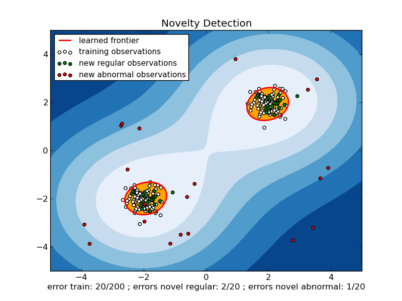
In general, it is about to learn a rough, close frontier delimiting
the contour of the initial observations distribution, plotted in
embedding  -dimensional space. Then, if further observations
lay within the frontier-delimited subspace, they are considered as
coming from the same population than the initial
observations. Otherwise, if they lay outside the frontier, we can say
that they are abnormal with a given confidence in our assessment.
The One-Class SVM has been introduced in [1] for that purpose and
implemented in the Support Vector Machines module in the
svm.OneClassSVM object. It requires the choice of a
kernel and a scalar parameter to define a frontier. The RBF kernel is
usually chosen although there exist no exact formula or algorithm to
set its bandwidth parameter. This is the default in the scikit-learn
implementation. The  parameter, also known as the margin of
the One-Class SVM, corresponds to the probability of finding a new,
but regular, observation outside the frontier.
Examples:
- See One-class SVM with non-linear kernel (RBF) for visualizing the frontier learned around some data by a svm.OneClassSVM object.
2.7.2. Outlier Detection
Outlier detection is similar to novelty detection in the sense that the goal is to separate a core of regular observations from some polluting ones, called “outliers”. Yet, in the case of outlier detection, we don’t have a clean data set representing the population of regular observations that can be used to train any tool.
2.7.2.1. Fitting an elliptic envelop
One common way of performing outlier detection is to assume that the regular data come from a known distribution (e.g. data are Gaussian distributed). From this assumption, we generally try to define the “shape” of the data, and can define outlying observations as observations which stand far enough from the fit shape.
The scikit-learn provides an object covariance.EllipticEnvelope that fits a robust covariance estimate to the data, and thus fits an ellipse to the central data points, ignoring points outside the central mode.
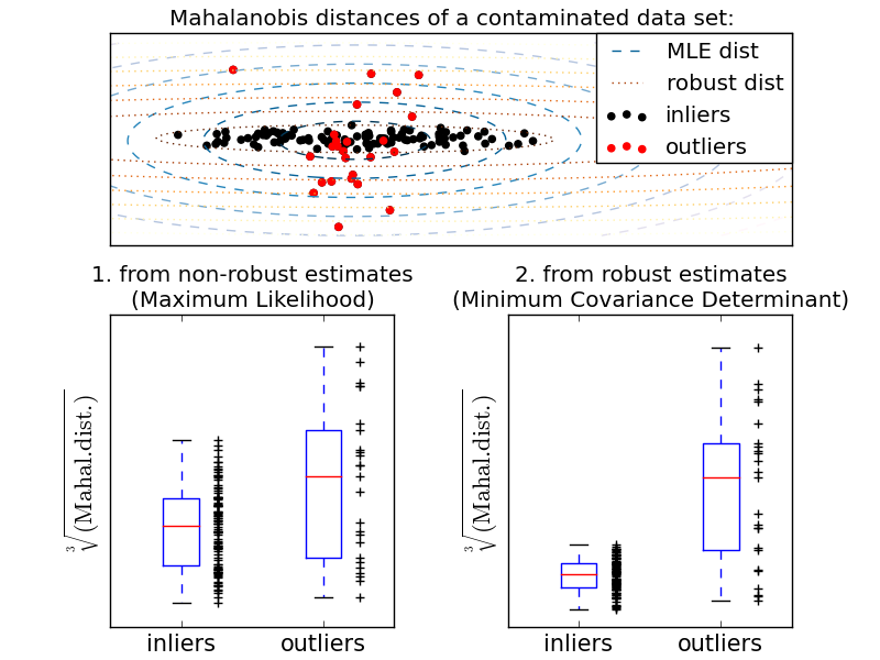
For instance, assuming that the inlier data are Gaussian distributed, it will estimate the inlier location and covariance in a robust way (i.e. whithout being influenced by outliers). The Mahalanobis distances obtained from this estimate is used to derive a measure of outlyingness. This strategy is illustrated below.
Examples:
- See Robust covariance estimation and Mahalanobis distances relevance for an illustration of the difference between using a standard (covariance.EmpiricalCovariance) or a robust estimate (covariance.MinCovDet) of location and covariance to assess the degree of outlyingness of an observation.
References:
| [RD1999] | Rousseeuw, P.J., Van Driessen, K. “A fast algorithm for the minimum covariance determinant estimator” Technometrics 41(3), 212 (1999) |
2.7.2.2. One-class SVM versus elliptic envelop
Strictly-speaking, the One-class SVM is not an outlier-detection method, but a novelty-detection method: it’s training set should not be contaminated by outliers as it may fit them. That said, outlier detection in high-dimension, or without any assumptions on the distribution of the inlying data is very challenging, and a One-class SVM gives useful results in these situations.
The examples below illustrate how the performance of the covariance.EllipticEnvelope degrades as the data is less and less unimodal. svm.OneClassSVM works better on data with multiple modes.
| For a inlier mode well-centered and elliptic, the svm.OneClassSVM is not able to benefit from the rotational symmetry of the inlier population. In addition, it fits a bit the outliers present in the training set. On the opposite, the decision rule based on fitting an covariance.EllipticEnvelope learns an ellipse, which fits well the inlier distribution. | 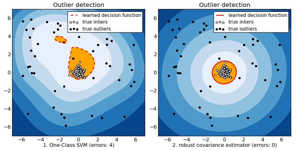 |
| As the inlier distribution becomes bimodal, the covariance.EllipticEnvelope does not fit well the inliers. However, we can see that the svm.OneClassSVM tends to overfit: because it has not model of inliers, it interprets a region where, by chance some outliers are clustered, as inliers. | 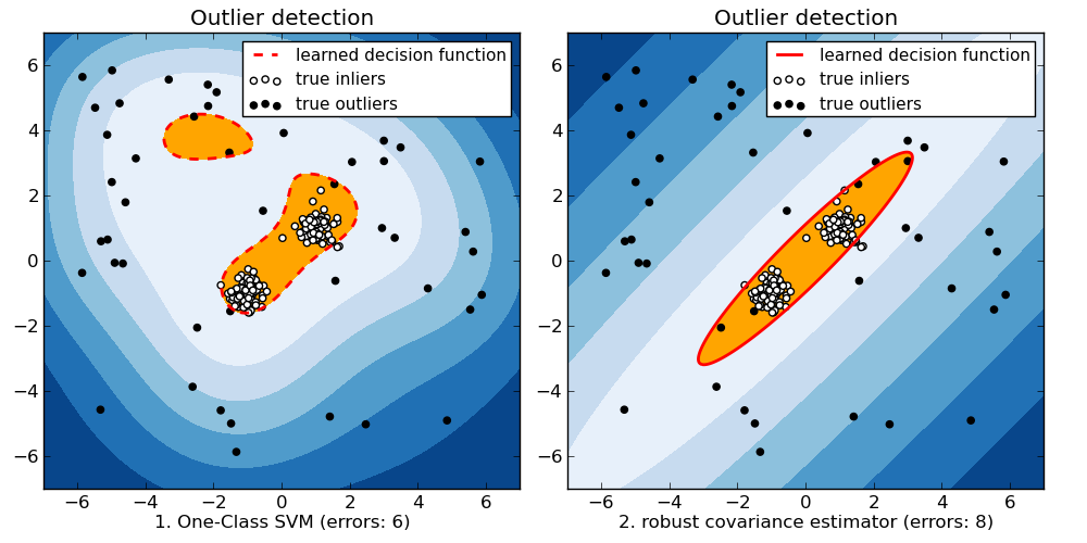 |
| If the inlier distribution is strongly non Gaussian, the svm.OneClassSVM is able to recover a reasonable approximation, whereas the covariance.EllipticEnvelope completely fails. | 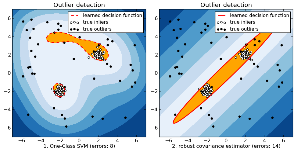 |
Examples:
- See Outlier detection with several methods. for a comparison of the svm.OneClassSVM (tuned to perform like an outlier detection method) and a covariance-based outlier detection with covariance.MinCovDet.


