Deep Learning for Forecasting in R: an Honest Guide
Deep learning for forecasting means turning a time series into an ordinary table of past-value columns, then training a network of simple "bend the number" units to predict the next value. This page builds one from scratch in R so you can watch it learn, then does the thing most tutorials skip: it scores the network against plain regression and ARIMA on the same data, with the same metric. Sometimes the network wins by a whisker. Twice it loses. Every number below was measured by running the code, not estimated, and you can run all of it right here.
What happens when you point a neural network at a time series?
Before any theory, let us settle the only question that matters: does a neural forecaster actually beat the simple methods you already know? We will race three things on the same data. The first is nnetar(), a ready-made neural network forecaster from the forecast package. The second is auto.arima(), the classical workhorse. The third is a deliberately dumb rule we will call the "no-model" baseline: predict next month by simply repeating this month's value. That last one is not a joke. If your fancy model cannot beat "tomorrow looks like today," it has earned nothing.
We will forecast monthly sunspot counts. The sunspot.month series ships with R and records how many sunspots were seen each month. It rises and crashes on a roughly eleven-year cycle, the rises are steeper than the falls, and that lopsided shape is exactly the kind of nonlinearity a straight-line model struggles with. It is the fairest possible home turf for a network. We train on 1900 through 1959 and test on 1960 through 1983, so every model is judged on years it never saw. Press Run.
The fitted(..., model = ...) calls keep the weights learned from 1900 to 1959 and only apply them to the later months, so no test value ever changed how a model was trained. That is what lets us score all three on years none of them were fitted on.
Those three numbers are mean absolute error (MAE): on average, how many sunspots each model was off by, per month, across the 1960 to 1983 test years. Smaller is better. Read them slowly. The neural network scored 18.05. ARIMA scored 17.87. The no-model baseline scored 19.16.
The network beat "repeat last month" by about one sunspot per month. ARIMA, a method from the 1970s with no neurons anywhere, beat the network. This is the honest starting point of the whole page, and it is nothing like the "deep learning crushes the classics" headline you may have expected. Hold onto that surprise; by the end you will know exactly why it happens and when it flips.
Let us look at what we are actually forecasting before we build anything.
We have 1008 months in total: 720 for training and 288 for testing. The counts run from 0 in quiet years to 359 at the peak of a busy cycle, with a typical month around 76. A picture makes the cycle obvious.
The dashed line marks 1960, where training ends and testing begins. Notice the repeating boom-and-bust cycles and how the peaks vary in height. A model has to learn both the rough rhythm and the fact that no two cycles are identical. That is genuinely hard, which is why the scores are so close together.
Try it: The no-model baseline depends on where you cut the data. The block below cuts at 1950 and re-scores "repeat last month" on the test years. Run it, then open the solution to see the same thing at a 1970 cut.
Click to reveal solution
Explanation: The baseline MAE changes with the test window (20.26 versus 21.69) because different years contain different amounts of month-to-month jumpiness. This is exactly why a fixed train/test split matters: change the split and every score shifts, so all models must be compared on the identical split.
How do you turn a time series into a table a network can read?
A neural network does not understand "time." It understands rows of a table: a set of input numbers, and a target number to predict. So the first real job in neural forecasting has nothing to do with neurons. It is reshaping the series into a supervised table, where each row says "given these recent values, predict the next one."
The trick is lagging. To predict a given month, we hand the network the previous twelve months as twelve input columns. The value from one month ago becomes column lag1, from two months ago lag2, and so on to lag12. The value we want to predict is the target. Slide this twelve-month window forward one step at a time and every month in the series becomes one training row.
Look closely at how the rows connect. In the first row the target is 257.7. In the very next row, that same 257.7 has slid into the lag1 column, because from the second row's point of view it is now "last month." Each target becomes the next row's most recent input. That sliding is the entire idea: we have taken a one-dimensional series and rewritten it as a normal predict-the-target table, the kind any regression tool can fit.
There is one more step before a network can use this, and skipping it is the single most common beginner mistake. Neural networks train far better when every input sits in a small, tidy range, so we rescale the counts to lie between 0 and 1. The catch: we must compute the minimum and maximum using the training years only, then apply those same two numbers to the test years. If we peeked at the test data to set the scale, we would be leaking future information into training, and our test score would be a flattering lie.
The training years span 0 to 359.4 sunspots, so we divide everything by that range. After reshaping we have 708 training rows and 288 test rows, each with 12 input columns and one target. That table, tr for training and te for testing, is what every model on this page will learn from. Figure 1 shows the shape of what we are about to build on top of it.

Figure 1: How twelve lagged months become one forecast.
Try it: We used 12 lags. The block below rebuilds the input table with only 6 lags. Run it and note how many usable training rows you get, then open the solution to see 24 lags.
Click to reveal solution
Explanation: More lags means each row needs more history to exist, so you lose usable rows off the front of the series: 714 rows at 6 lags, 696 at 24 lags. More inputs also means more weights to fit from fewer examples, which is a trade-off we will feel later.
How do you build and train a network from scratch in base R?
Now the neurons. The word "network" sounds intimidating, so let us defuse it. A single neuron does two tiny things: it takes a weighted sum of its inputs, then it bends that sum through a smooth squashing function. That is all. Here is one neuron, by hand, using twelve random weights and one row of our table.
The neuron multiplied each of the twelve lagged values by its own weight, added them up along with a bias term, and got 0.1722. Then it passed that through tanh, a function that gently squashes any number into the range from -1 to 1, giving 0.1705. That squashing is what lets a network learn bends instead of straight lines, so it can follow curves and asymmetric rises and falls. Here is the shape of tanh at a few points.
Notice how tanh is nearly straight through the middle (near 0 it barely changes the number) but flattens out at the edges: big positive inputs all get squashed toward 1, big negative ones toward -1. A layer of these neurons, each with its own weights, can bend the inputs in different places, and a final neuron adds up their bends into one forecast. Written as formulas, each hidden neuron $j$ computes
$$h_j = \tanh\left(\sum_{i=1}^{12} w_{ij}\, x_i + b_j\right)$$
and the output combines them into a prediction
$$\hat{y} = \sum_{j} v_j\, h_j + c$$
Where $x_i$ are the twelve lagged inputs, $w_{ij}$ and $b_j$ are the weights and bias of hidden neuron $j$, $v_j$ and $c$ are the output weights and bias, and $\hat{y}$ is the forecast. If the math is not your thing, skip it: the code below is the same idea and is all you need.
Let us write the network as two small functions. init_net creates random starting weights for whatever layer sizes we ask for. forward runs a table of inputs through the network to get predictions. We check the untrained network's error first, so we have something to improve on.
We built a network with 12 inputs, 8 hidden neurons, and 1 output, all starting from random weights. Its mean squared error on the training rows is 0.2622, which is terrible, as expected: random weights predict nonsense. Training is the process of nudging those weights until the error shrinks.
The nudging rule is called gradient descent, and it is more intuitive than its name. Each round, called an epoch, we do four things: run every row forward to get predictions, measure how wrong they are, work out which direction to shift each weight to reduce the error (that backward calculation is "backpropagation"), and take a small step in that direction. Repeat a few thousand times. The step size is the learning rate. Figure 2 shows the loop.
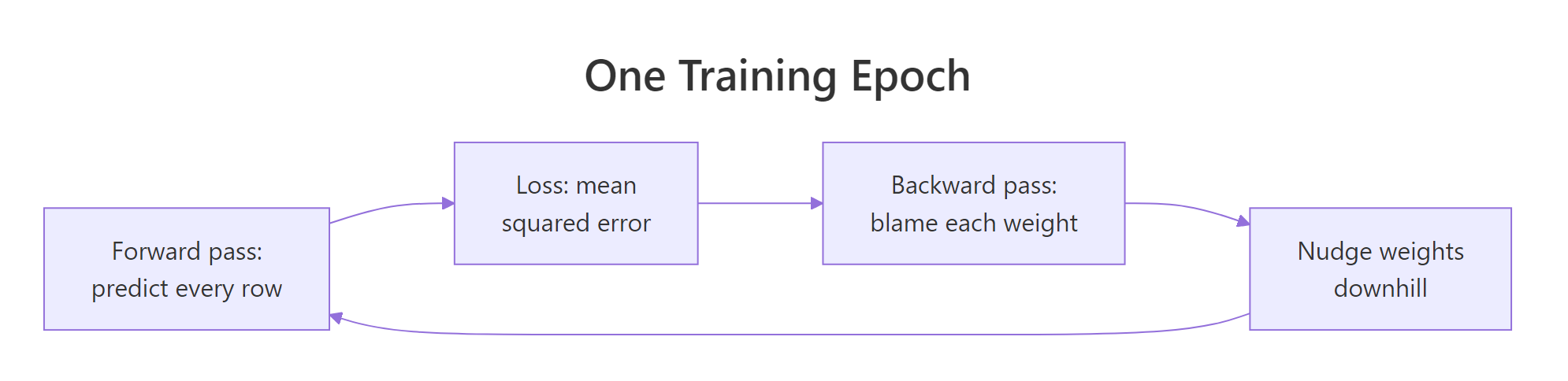
Figure 2: One epoch: predict, measure, assign blame, nudge.
The loss we are shrinking is the mean squared error between predictions and targets, and each weight moves against its slope:
$$L = \frac{1}{n}\sum_{t=1}^{n}(\hat{y}_t - y_t)^2 \qquad w \leftarrow w - \eta\, \frac{\partial L}{\partial w}$$
Where $\eta$ is the learning rate. Here is the whole training loop in R. It is under twenty lines, and it is complete: no deep learning library, just matrix arithmetic.
Watch the training error fall: 0.2622 at the start, down to 0.00627 after 100 epochs, then slowly settling near 0.0054. The steep early drop is the network learning the obvious pattern; the long flat tail is it squeezing out the last bits. After 3000 epochs it has stopped improving, so we stop. We now have a trained network. Let us score it on the test years against the same rivals from the opening, remembering to convert predictions back to the original sunspot scale.
Our hand-built network scored 17.52, edging out both nnetar (18.05) and ARIMA (17.87). That feels like a win for deep learning. But before you celebrate, we have to run the test that separates real skill from wishful thinking: how does the network compare to plain linear regression fed the exact same twelve lag columns? Linear regression has no hidden layer, no tanh, no epochs. If the network cannot beat it, the neurons added nothing.
Linear regression scored 17.75. The network scored 17.52. The neural network, with its hidden layer and thousands of training epochs, beat a one-line linear model by 0.23 sunspots per month, about one percent. That is the honest size of the "deep learning advantage" on this series. It is real, but it is tiny, and you should now be deeply suspicious of any tutorial that reports a huge neural win without ever showing you the linear baseline.
lm() was about one percent. Neurons shine when the pattern is genuinely nonlinear and you have lots of data, not on one modest series where a straight line already captures most of the signal.Try it: The learning rate controls how big each downhill step is. The block below trains at a cautious lr = 0.05 and reports a slow descent. Run it, then open the solution to see what a reckless lr = 2 does.
Click to reveal solution
Explanation: At lr = 0.05 the loss falls slowly but steadily. At lr = 2 each step overshoots the bottom of the valley and bounces higher every time, so the weights race off to infinity and the error becomes NaN. The learning rate is the most sensitive knob you have: too small wastes time, too large destroys the model.
Does adding more layers make the forecast better, or just noisier?
"Deep" learning suggests that more layers means more power. Let us test that belief directly by adding a second hidden layer and re-scoring. Everything else stays the same.
The two-layer network scored 17.54; the one-layer network scored 17.52. Adding a whole extra layer of neurons made the forecast very slightly worse. That 0.02 difference is not a meaningful gap in either direction, which raises an uncomfortable question: how much of any of these scores is just luck from the random starting weights? We can measure that directly by training the same network six times with six different random seeds.
Here is the result that should reshape how you read every neural forecasting claim. The same network, same data, same settings, scored anywhere from 17.53 to 19.07 depending only on the random seed. The spread is 1.54 sunspots. Now recall the one-layer versus two-layer difference: 0.02. The effect of adding a layer was seventy times smaller than the noise from simply re-rolling the dice on the starting weights.
This is why serious neural forecasting always averages several networks, which is exactly what nnetar's repeats argument does under the hood. It is not a nicety; it is the difference between a reproducible number and a coin flip.
Try it: Does making the hidden layer wider help? The block below trains a 16-neuron network. Run it, then open the solution to see a tiny 2-neuron network.
Click to reveal solution
Explanation: Sixteen neurons (17.64) and two neurons (17.81) both land within the seed-noise band around the eight-neuron model (17.52). On this series, width barely matters. The pattern is simple enough that a small network already captures it, and extra capacity mostly adds wiggle room to overfit.
Does the network still win when you forecast further than one step?
So far every score was one-step-ahead: predict next month given the true last twelve months. Real forecasting rarely stops there. You usually need the next year, twelve months out, and you do not get to peek at the true values in between. You have to feed the model's own predictions back in as inputs. This is recursive forecasting, and it is where errors can snowball.
We roll through the test years, and at each starting point we forecast twelve months ahead by feeding predictions back into the network. We compare the network against ARIMA and the no-model baseline. To keep the comparison fair, we use twenty-four separate starting points across the test period.
Two things jump out. First, every error is bigger than the one-step numbers: forecasting twelve months out is simply harder, so MAE climbs from around 18 to the high 20s. Second, and more interesting, the ranking changed. Over a twelve-month horizon the network (27.09) now beats ARIMA (30.27) and edges past the no-model baseline (28.80). The network's ability to bend around the cycle pays off more when it has to project a whole year of ups and downs rather than a single next step.
There is a second way to forecast twelve months out: train a network specifically to predict the value twelve months ahead in one shot, rather than stepping to it. That is the "direct" strategy. Let us pit direct against recursive at exactly the twelve-month mark.
At the twelve-month mark specifically, recursive (34.51) slightly beat direct (35.67), and both beat doing nothing (38.43). Here we used nnet, R's built-in single-hidden-layer network, to build the direct model in one line, which is a handy shortcut when you do not want to hand-roll the training loop. Neither strategy is universally best; the choice depends on your horizon and how much error compounds.
Try it: Does the network's edge hold at a shorter horizon? The block below scores the recursive network six months out. Run it, then open the solution for a two-year horizon.
Click to reveal solution
Explanation: At six months the network leads the baseline by a little (23.14 versus 24.53); at twenty-four months its lead widens (36.58 versus 43.92). The longer the horizon, the more the network's grasp of the cycle beats blindly repeating the last value, because a flat line drifts ever further from a series that keeps oscillating.
When does deep learning actually win?
We have been fair to the network and it has been unremarkable: a whisker better than linear regression on one series. So when does deep learning genuinely earn its keep? The answer, and it is the central lesson of modern forecasting, is when you have many related series and train one network across all of them at once. A network with only one short series to learn from behaves very differently from one trained on thousands of examples drawn from a whole population of series.
Let us simulate that. Imagine forty shops, each with a short sales history that follows the same underlying boom-bust dynamic but with its own noise. No single shop has much data, but together they reveal the shared rule. We will forecast one focus shop two ways: a network trained on that shop alone, versus a network trained on all forty shops pooled together.
One shop gives us 34 training rows, barely enough to fit anything reliably. Pooling all forty shops gives 1360 rows of the same underlying pattern. Each shop is short, but the pattern they share is now richly sampled. Now we train the solo network, the pooled network, and, to keep ourselves honest, a linear model on the same pooled data.
This is the payoff of the whole page. The network trained on a single shop scored 0.119. The very same network trained on all forty shops scored 0.068, almost twice as accurate. And crucially, a linear model given the identical pooled data managed only 0.221, because the boom-bust rule is genuinely curved and a straight line cannot follow it. Here, at last, the network is not beating linear regression by one percent. It is nearly three times better, and the pooled network beats the solo network by a wide margin too.
This mirrors the real evidence. In the M4 competition of 2018, across 100,000 mostly single series, pure machine learning methods did poorly and classical statistics dominated; the one neural method that won was a hybrid glued to exponential smoothing. Two years later in the M5 competition, forecasting thousands of related Walmart sales series, machine learning swept the board. The deciding factor was not smarter neurons. It was many related series to learn across.
Try it: How many shops do you need before pooling helps? The block below pools just 5 shops. Run it, then open the solution for 20 shops.
Click to reveal solution
Explanation: Five shops (0.078) already beats the single-shop network (0.119), and twenty shops (0.068) matches the full forty-shop result. The gain from pooling is steep at first and then flattens: even a handful of related series helps a lot, and you hit diminishing returns well before you need hundreds.
What are your real deep learning options in R today?
You now understand the machinery, so let us map it to the tools you would actually reach for. You rarely hand-code backpropagation in practice; you did it here to demystify it. In real work you pick a package sized to the job.
| Tool | What it is | Reach for it when |
|---|---|---|
nnetar() (forecast) |
One-line neural autoregression, auto-averaged | You want a neural baseline in seconds on one series |
nnet |
Base single-hidden-layer network | You want a direct multi-step forecaster fast |
torch |
Native R deep learning, no Python | You need LSTMs, GRUs, or custom architectures |
keras3 |
R interface to Keras/TensorFlow | You prefer the Keras style or port Python models |
modeltime |
Tidy wrapper unifying many forecasters | You want neural and classical models side by side |
For anything beyond a plain feed-forward network, torch is the modern choice in R. It runs natively without Python and gives you recurrent layers such as LSTMs, which carry a memory across time steps rather than seeing a fixed window of lags. A minimal torch model for our lag table looks like this. It will not run in your browser here (deep learning frameworks need to be installed on your own machine), so treat it as a sketch to run locally.
# Run this locally after install.packages("torch")
library(torch)

net <- nn_module(
  initialize = function() {
    self$fc1 <- nn_linear(12, 8)
    self$fc2 <- nn_linear(8, 1)
  },
  forward = function(x) x |> self$fc1() |> nnf_tanh() |> self$fc2()
)
model <- net()
opt   <- optim_adam(model$parameters, lr = 0.01)
# ... training loop: forward, loss, backward, step ...
That is the identical structure you built by hand: a linear layer, a tanh bend, another linear layer. torch just handles the gradients and speed for you. Whatever tool you choose, the discipline stays the same: always check the network against a linear model and a naive baseline before you trust it. Let us wrap that discipline into a reusable function.
Read this table carefully, because it is the most useful thing on the page. On sunspots and nottem (monthly temperatures) the network wins, but only just, over linear regression. On AirPassengers the network (18.48) loses badly to linear regression (15.72), because that series is a smooth trend where a straight line already excels and the network merely adds noise. On UKDriverDeaths the network (135.67) barely beats the no-model baseline and loses to linear regression again. Two wins, two losses. That is the real batting average of a plain neural forecaster on ordinary single series, and it is why "just throw deep learning at it" is bad advice. Figure 3 turns this into a decision you can follow.
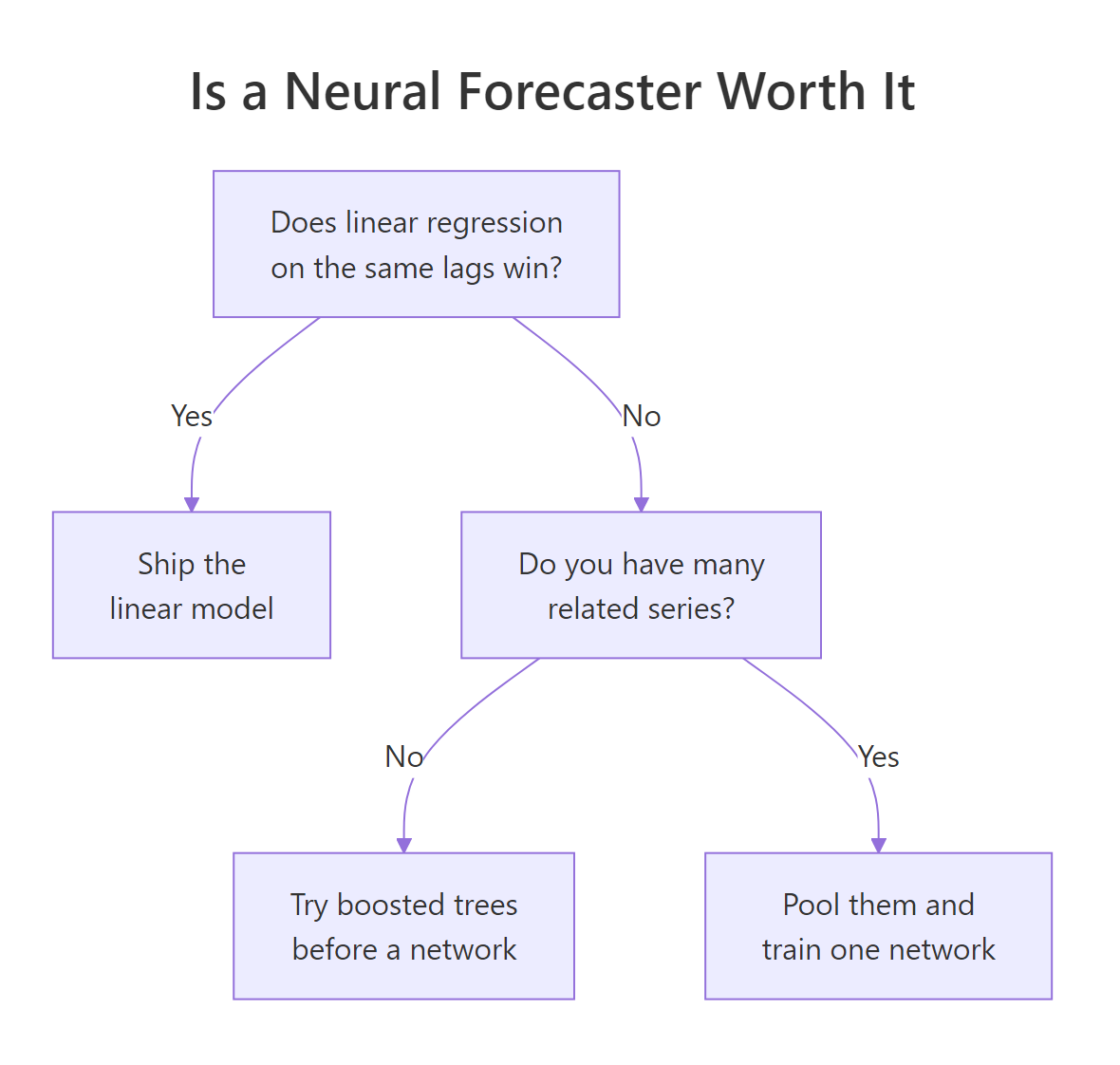
Figure 3: When a neural forecaster is worth the trouble.
worth_it() a habit, not an afterthought. Run every candidate network against linear regression and the naive baseline on your own data before you deploy it. If the network does not clearly beat both, ship the simpler model: it is faster and easier to explain, and it gives the same answer every time.Try it: Run the honesty check on a new series. The block below scores the lynx series (annual lynx trappings), using 6 lags since it is annual. Run it, then open the solution for BJsales.
Click to reveal solution
Explanation: On lynx, a wildly nonlinear predator-prey cycle, the network (639.25) genuinely beats linear regression (666.68): this is the kind of series neurons are built for. On BJsales, a smooth near-random-walk, the network (2.08) is more than twice as bad as simply repeating the last value (0.91). Same code, opposite verdicts. The series decides, not the algorithm.
Complete Example: an honest neural forecast from start to finish
Here is the entire workflow in one block: split the data, scale on training only, train the network, score it against both baselines, and print a plain-English verdict. This is the template to copy for your own series.
On the sunspot series with an 80/20 split the network scored 19.50, just ahead of linear regression at 19.67, so the verdict is to keep it, though by a margin thin enough that you would want several seeds before trusting it. The function does not care about the answer; it just reports whether the network earned its complexity. Swap in your own series and it will tell you, honestly, whether deep learning is worth it.
Practice Exercises
These combine the ideas above. Each starter block runs as-is so you can experiment; reveal the solution only after you have tried.
Exercise 1: Does the network win on the training-era sunspots alone?
Score the network against both baselines on just the 1900 to 1959 stretch of sunspots (720 months). Use worth_it() with 12 lags and read which column is smallest. Is the verdict a win or a loss?
Click to reveal solution
Explanation: On this shorter slice the network (23.42) loses to both linear regression (21.60) and, embarrassingly, is worse than the full-series result. Less data means the network overfits its limited training rows and generalizes worse. The verdict here is to ship the simpler model, a reminder that more neurons cannot rescue a data shortage.
Exercise 2: How does lag depth change the verdict?
Sweep the number of lags across 3, 6, 12, and 24 on the full sunspot series and stack the worth_it() rows into one table. Does giving the network more history (more lags) ever turn a loss into a win against linear regression?
Click to reveal solution
Explanation: The network beats linear regression at every lag depth here, and its edge grows slightly with more lags (18.65 at 3 lags down to 18.27 at 24 lags) because the eleven-year cycle needs a long memory to capture. But every gap is small and within seed noise, so the practical takeaway is that lag depth matters more than architecture on this series.
Exercise 3: Find the best stopping point with a validation split
Training too long overfits. Hold out the last 24 of the first 80 training rows as a validation set, train in chunks of 300 epochs, and track the validation error after each chunk. At which epoch is validation error lowest? Training past that point is wasted effort or worse.
Click to reveal solution
Explanation: Training error (fit_mse) keeps falling forever, but validation error bottoms out at 900 epochs and then climbs. Past that point the network is memorizing the training rows, not learning the pattern, which hurts on unseen data. Stopping when validation error turns upward, called early stopping, is one of the most important guards against overfitting a neural forecaster.
Frequently Asked Questions
Is deep learning always better than ARIMA for forecasting? No, and this page proves it with numbers. On a single ordinary series, ARIMA and even plain linear regression frequently match or beat a neural network. Deep learning pulls ahead when the pattern is strongly nonlinear or when you can train one model across many related series, as in the forty-shop example.
Do I need a GPU to forecast with neural networks in R? Not for the models here. Everything on this page trained in seconds on a plain laptop using nothing but base R matrix arithmetic. GPUs matter for large torch or keras3 networks with recurrent layers and thousands of series, not for a modest feed-forward forecaster.
What is the difference between nnetar and a torch LSTM? nnetar() fits a simple feed-forward network on lagged inputs, the same design you built by hand, and averages several of them. A torch LSTM adds a memory that carries state across time steps instead of seeing a fixed window of lags, which can help on long or complex sequences but needs more data and tuning to pay off.
Why did my neural forecast give a different number each time I ran it? Because the starting weights are random. As the six-seed experiment showed, the same network can vary by more than a full point of MAE from run to run. Set a seed for reproducibility and average several networks before you trust any single score.
How much data do I need before deep learning is worth trying? As a rough guide, you want far more training rows than network weights. A single short series rarely qualifies. If you have dozens or hundreds of related series, pool them into one model, and that is exactly when neural methods start to shine.
Summary
| Takeaway | What the numbers showed |
|---|---|
| Always compare to a baseline | The network beat "repeat last month" (19.16) by barely one point |
| Neurons barely beat regression on one series | 17.52 network versus 17.75 linear, about one percent |
| Depth is inside the noise | One versus two layers differed by 0.02; seed noise was 1.54 |
| Average several seeds | A single run could land anywhere from 17.53 to 19.07 |
| Deep learning wins by pooling series | Pooled network 0.068 versus solo network 0.119 |
| The series decides, not the algorithm | Two wins and two losses across four real series with worth_it() |
| Stop training early | Validation error bottomed at 900 epochs, then rose |
Deep learning is a genuine tool in the forecasting toolbox, not a magic upgrade. You built one from scratch, watched it learn, and scored it fairly: it earned a small win on some series and an honest loss on others. The habit that will serve you longest is not any architecture, it is the reflex to always race your network against a naive baseline and a linear model before you believe it.
References
- Hyndman, R.J. & Athanasopoulos, G. - Forecasting: Principles and Practice, 3rd Edition. Neural network models. Link
- Makridakis, S., Spiliotis, E. & Assimakopoulos, V. - The M4 Competition: results, findings, and conclusions. PLOS ONE (2018). Link
- Benidis, K. et al. - Deep Learning for Time Series Forecasting: Tutorial and Literature Survey (2020). Link
- Oreshkin, B. et al. - N-BEATS: Neural basis expansion analysis for interpretable time series forecasting (2019). Link
- torch for R - official documentation. Link
- Keydana, S. - Introductory time-series forecasting with torch. Posit AI Blog. Link
- Hyndman, R.J. -
nnetar()function reference, forecast package. Link - keras3 for R - official documentation. Link
- Venables, W.N. & Ripley, B.D. -
nnet: Feed-forward neural networks. CRAN. Link
Continue Learning
- Gradient Boosting for Time Series in R - the tree-based method that actually swept the M5 competition, built from scratch the same way.
- Global Forecasting Models in R - the pooling idea from section 6, done properly on real retail data.
- Backtesting Forecast Models in R - rolling-origin evaluation so your scores never fool you.