What the M Competitions Teach About Forecasting
The M competitions are a series of large, open forecasting contests, run by Spyros Makridakis since 1982, that test which methods actually predict the future best. Their verdicts have shaped modern practice: simple methods are hard to beat, combining forecasts reliably helps, and you must judge accuracy honestly on data the model never saw. This tutorial reproduces those lessons in a few lines of R so you can watch them happen.
Instead of taking these findings on faith, we are going to run miniature versions of the competitions ourselves. Every claim below comes with runnable code, so by the end you will have your own tiny forecasting bake-off that you can point at any series. We use the classic forecast package throughout because it gives us every method and every score in one place.
What are the M competitions, and why should you care?
A forecasting competition works like a fair exam. Everyone gets the same history, hides the most recent stretch, forecasts it, and then scores those predictions against what really happened. The M competitions did this at massive scale and settled decades of arguments with evidence instead of opinion. We start by running that exact test on a single series so the mechanic is concrete before anything else.
Here is the whole idea in one block. We take the monthly airline passengers series that ships with R, hide the last two years, forecast them with a deliberately dumb method, and score the result. The dumb method is the "seasonal naive" forecast: it simply predicts that each month will match the same month one year earlier.
That tiny block is the entire M-competition machine in miniature. We split the series into a training set (the model is allowed to see it) and a test set (kept hidden). We forecast 24 months ahead with snaive(), then accuracy() compares the forecast to the hidden test values and reports three error scores. Smaller scores mean a better forecast. We now have a number to beat, MAPE of 15.52 percent, and every method later in this post will be judged the same fair way.
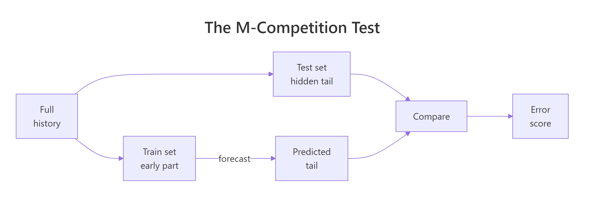
Figure 1: The M-competition test: hide the tail of a series, forecast it, then score the prediction against what actually happened.
The competitions grew enormously over four decades. The table below is your map for the rest of the post: each row is one competition, and the last column is the headline result we will reproduce or explain.
| Competition | Year | How many series | Headline result |
|---|---|---|---|
| M1 | 1982 | 1,001 | Simple methods do as well as complex ones |
| M2 | 1993 | 29 (real time) | Confirmed M1 on live data |
| M3 | 2000 | 3,003 | The simple Theta method won |
| M4 | 2018 | 100,000 | A stats-plus-machine-learning hybrid won |
| M5 | 2020 | 42,840 (retail) | Gradient-boosted trees won |
Try it: Set up your own hold-out on a different series. Split the USAccDeaths monthly series so the training set ends in December 1977 and the test set is all of 1978, then confirm the test set has 12 months.
Click to reveal solution
Explanation: window() slices a time series by calendar position. Ending the training set in December 1977 and starting the test set in January 1978 leaves exactly the 12 months of 1978 to forecast.
Why do simpler methods so often win?
The most famous finding of the M competitions is uncomfortable for anyone who loves complicated models: statistically sophisticated methods do not automatically forecast better than simple ones. To see it, we pit four methods against each other on the same hold-out. Here is a one-line description of each, in plain language, before we run anything:
- Seasonal naive: repeat last year's value for each month. The floor everything must beat.
- ETS: exponential smoothing, a weighted average that leans on recent months and tracks trend and season.
- ARIMA: an autoregressive model that predicts each point from recent points and recent errors.
- Theta: the strikingly simple method that won the M3 competition, built from just two smoothed lines.
We fit all four to the same train, forecast the same 24 months, and score them with one helper so the comparison is airtight. The helper computes three errors we will lean on: MASE, RMSE, and MAPE (we unpack what each means in a later section).
Read the table one row at a time. The $mean inside each forecast object is the vector of 24 predicted values, and score() turns each vector into three error numbers. Lower is better in every column, so scan down each column for the smallest value.
The result is exactly the M-competition story. The two simplest methods, ETS and Theta, post the lowest errors. The more elaborate ARIMA lands behind both of them, and the seasonal naive baseline is the worst, as expected. Nothing here says complex models are bad; it says complexity has to earn its keep against a simple, well-chosen alternative, and here it did not.
Try it: How much does ignoring seasonality cost? Forecast the same train with the plain, non-seasonal naive() (it just repeats the very last value forever) and score it with our score() helper.
Click to reveal solution
Explanation: Plain naive() repeats the final observed value, so it flatlines and misses every seasonal swing. Its MASE of 4.03 is far worse than the seasonal naive's 2.49, which is why seasonal naive, not plain naive, is the honest benchmark for seasonal data.
Does combining forecasts really beat the best single method?
If the M competitions have one signature lesson, this is it: instead of agonising over which single model to trust, average several of them. A combined forecast is often more accurate than the individual forecasts inside it, and it is almost always safer. Let us test that claim directly by averaging our three real models, point by point, into one forecast.
We added one row to the table. fc_combo is just the arithmetic mean of three forecast vectors, and we scored it exactly like the others. Now compare that new bottom row to the four above it.
Notice what the combination did and did not do. It did not top the table on this single series; Theta edged it out on RMSE, and ETS tied Theta on MASE. But look again: the combination beat ARIMA and the seasonal naive on every metric, and it was never the worst at anything. That is the real prize. You would have needed to know in advance that Theta was the star to beat the average, and in practice you never know that in advance.
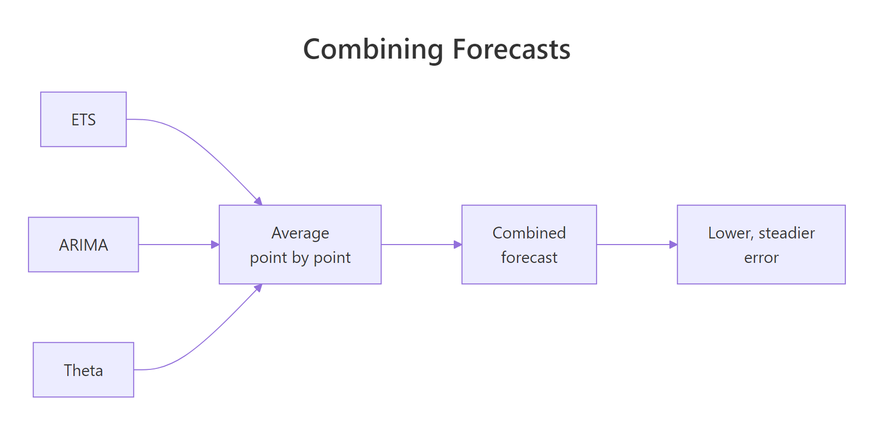
Figure 2: Combining forecasts: average several models point by point for a lower, steadier error.
Why does averaging help at all? Different models make different mistakes. ETS might overshoot in a month where ARIMA undershoots, so when you average them the errors partly cancel. It is the same reason a diversified portfolio is steadier than any single stock: you are not trying to pick the winner, you are smoothing out the losers.
Try it: Combinations do not have to use three models. Build a two-model average of just ETS and Theta, then score it.
Click to reveal solution
Explanation: Averaging the two strongest members gives an RMSE of 71.92, a hair better than the three-model average here because the weaker ARIMA is left out. In general you will not know which members are strongest ahead of time, which is exactly why broad, equal-weight combinations are so reliable.
Why does the best method change with your error metric?
You may have noticed that "which method is best?" already had different answers in different columns. That is the third M-competition lesson: the ranking of methods depends on the accuracy measure you choose. Before we prove it, here is what each of our three metrics actually means, in plain terms.
- RMSE (root mean squared error) is the typical size of a miss, in the original units (passengers). Because it squares errors, it punishes a few large misses heavily.
- MAPE (mean absolute percentage error) is the average miss as a percentage of the actual value. It is easy to explain but behaves badly when actual values are near zero.
- MASE (mean absolute scaled error) divides your error by the error of a seasonal naive forecast. Below 1 means you beat that baseline; above 1 means you did worse.
MASE is the metric the M4 competition leaned on, precisely because dividing by a baseline makes it comparable across series of wildly different scales. If you like formulas, here is the intuition made exact. The top is your average miss on the test set; the bottom is the seasonal naive's average miss on the training set.
$$\text{MASE} = \frac{\frac{1}{h}\sum_{t=1}^{h} \left| y_t - \hat{y}_t \right|}{\frac{1}{n-m}\sum_{t=m+1}^{n} \left| y_t - y_{t-m} \right|}$$
Where:
- $y_t$ = the actual value, and $\hat{y}_t$ = your forecast for it
- $h$ = the number of forecast points (24 months here)
- $n$ = the length of the training set, and $m$ = the season length (12 for monthly data)
- the denominator is the training-set error of predicting each month from the same month a year earlier
If you are not interested in the formula, skip it: the code above already computed MASE as mean(abs(e)) / scale_mae, which is the same thing. Now let us rank all five methods under each metric and watch the winner move.
rank() turns each column of errors into positions, where 1 is best. Reading across the rows shows the same methods trading places depending on the yardstick. Under MASE, ETS and Theta tie for first (the 1.5 is the average of ranks 1 and 2 for a tie). Under RMSE, Theta alone is first. Under MAPE, ETS is first and Theta drops to second. The combination shifts too, from third on MASE to second on RMSE.
The practical takeaway is blunt: never let someone tell you a method is "the most accurate" without asking accurate by which measure. Pick the metric that matches the cost of your errors first, then rank methods. If a single huge miss would be a disaster, weigh RMSE; if you need a scale-free number to compare across many products, use MASE.
Try it: Ask the table a direct question. Which single method has the lowest RMSE?
Click to reveal solution
Explanation: results[, "RMSE"] pulls out the RMSE column, which.min() finds the row with the smallest value, and names() reports it. Theta wins on RMSE even though it only tied for first on MASE, which is the whole point of this section.
How does the forecast horizon change the answer?
There is a fourth lever the M competitions surfaced: how far ahead you forecast changes which method looks best. A model that nails next month may drift badly two years out, and vice versa. We can see this on the very same forecasts by scoring them over a short window and a long window separately.
We sliced each forecast vector into its first 6 points and its full 24 points, then measured RMSE on each slice. The two columns tell different stories. Over the first six months, ETS is clearly the most accurate at 28.3, with Theta second. Over the full two years, they swap: Theta takes first at 71.4 and ETS slips to second. The best method genuinely depends on the horizon you care about.
This is why a good evaluation always scores at the horizon you will actually use. If you plan production one month ahead, a two-year-average error is the wrong number to optimise, and it might steer you to the wrong model entirely.
Try it: Zoom in even further. Compute the ETS forecast's RMSE over just the first three months.
Click to reveal solution
Explanation: Restricting the index to 1:3 scores only the nearest three months, where ETS is at its sharpest (11.8) because short-term forecasts have less room to drift than long ones.
Does the lesson hold across many series, or did we get lucky?
Everything so far ran on one series. That is exactly the trap the M competitions were built to avoid: any method can win on a lucky example. The real power of the competitions came from averaging results over thousands of series, so a good method has to be good on average, not just on your favourite chart. Let us build a small version of that idea over seven built-in series.
We write one function that runs our whole mini-contest on any series, then apply it across a list. For each series it holds out the last 24 points, fits all four methods plus the combination, and returns their MASE (scaled per series so the numbers are comparable).
sapply() runs run_contest() on each series and t() turns the result into a tidy one-row-per-series table. Scan the columns and the core M-competition lesson is clear: no single method wins everywhere. ETS is superb on co2 (0.21) but the worst on gas (3.33), where Theta alone does well at 2.74. Every method has a series it is bad at.
Now collapse the table to a single verdict by averaging each method's MASE across all seven series. This is the miniature version of "average over thousands of series."
On average, ETS finishes first and the combination edges out Theta for second, with both well ahead of ARIMA and the seasonal naive baseline. The combination did not top the podium, but think about what it bought you: without knowing in advance that ETS would win, the combination still beat three of the four individual methods and came within a whisker of the best. It is the one choice you could have made up front with no risk of a disaster.
Try it: The combination is meant to be safe. On how many of the seven series does it beat the seasonal naive baseline?
Click to reveal solution
Explanation: The combination beats the naive baseline on 6 of the 7 series. The exception is gas, where a strong seasonal pattern makes the naive forecast unusually hard to beat, a healthy reminder that the benchmark is not a pushover.
What did M4 and M5 change: machine learning, hybrids, and cross-learning?
The lessons above come mostly from the first three competitions. The two most recent ones, M4 in 2018 and M5 in 2020, brought machine learning into the arena, and the results are worth understanding because they refined the classic lessons rather than overturning them.
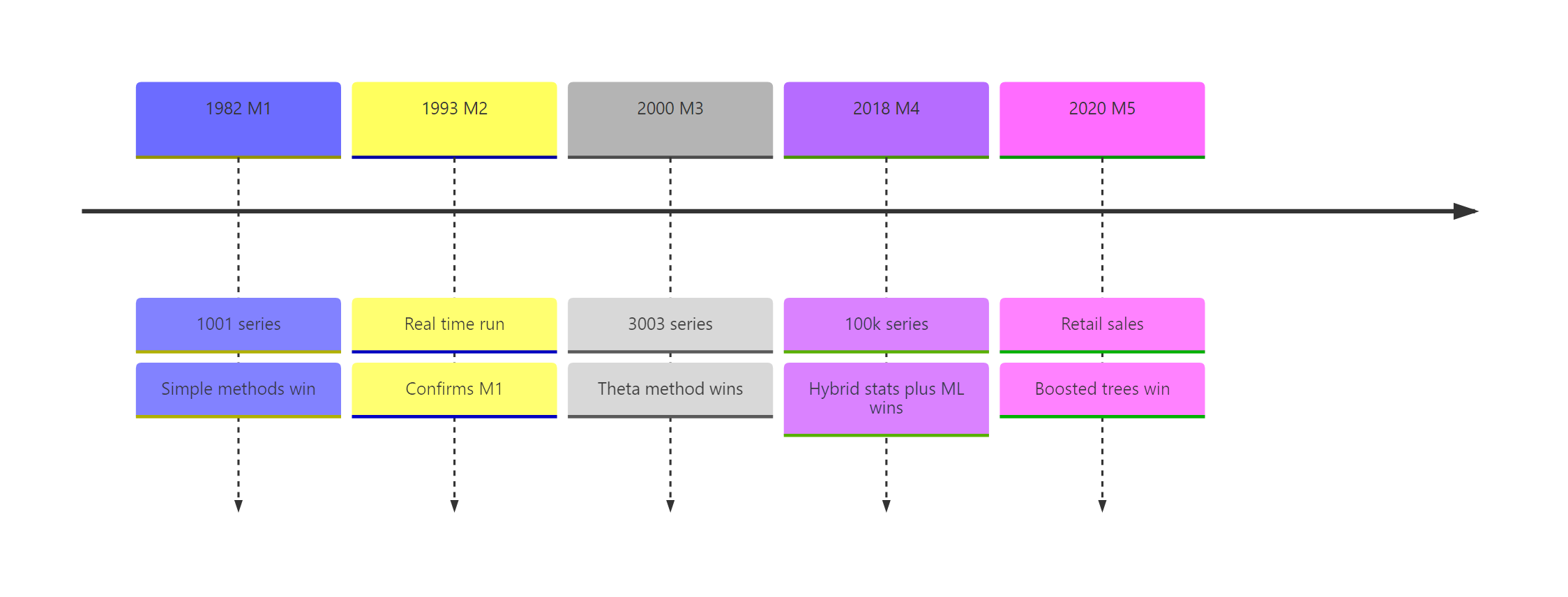
Figure 3: Five M competitions across four decades, and the headline result of each.
In M4 (100,000 series), the winner was a hybrid that bolted a neural network onto exponential smoothing, and second place went to a method called FFORMA that used machine learning to decide how to weight a pool of statistical models. The blunt subplot: pure machine-learning entries, with no statistical backbone, mostly did worse than the humble combination benchmark. Combining and cross-learning won; naive deep learning did not.
In M5 (Walmart retail sales), the story finally tilted toward machine learning. Gradient-boosted trees dominated both tracks. The difference was the data: M5 gave competitors thousands of related product series plus prices, promotions, and calendar events, and it rewarded models that learn across all series at once ("cross-learning") and forecast a whole distribution, not just a single number. With rich features and many related series, machine learning earned its complexity.
FFORMA's idea, choosing model weights from the shape of a series, is easy to make concrete. The feasts package measures features like how strong a series' trend and seasonality are, on a 0-to-1 scale. A method like FFORMA feeds exactly these numbers into a model that decides which forecasters to trust.
The airline series scores 0.99 for trend strength and 0.94 for seasonal strength, confirming what the eye sees: a strong upward trend plus a strong yearly cycle. A feature-based system measures dozens of series this way and learns, for example, to lean on seasonal methods when seasonal_strength_year is high. That is a combination that adapts to each series, and it is the through-line from the classic M lessons to the modern winners.
Try it: Measure the shape of a different series. Compute the trend and seasonal strength of the co2 series.
Click to reveal solution
Explanation: The atmospheric CO2 series has an almost perfect trend (1.000) and a very strong seasonal cycle (0.990), which is why the trend-and-season-aware methods like ETS did so well on it back in the seven-series contest.
Complete Example
To pull the whole idea into one reusable tool, here is a self-contained mini M-competition. Give it any seasonal series and a horizon; it holds out the tail, fits every method plus the combination, and returns a sorted MASE leaderboard. This single function is the practical distillation of everything above.
On the US accidental deaths series with a one-year hold-out, the combination comes out on top at 0.47, just ahead of ETS and ARIMA, with the seasonal naive baseline last. Point m_contest() at any series you like and you have run your own M competition: split, forecast, combine, score, and rank, all in one call.
Practice Exercises
These combine several ideas from the tutorial. Try each before opening the solution. They use my_ variable names so they will not disturb the objects we built above.
Exercise 1: Run the contest on a new series
Run a mini-contest on the fdeaths series (monthly female lung-disease deaths). Hold out the last 12 months, forecast with ETS and Theta, build their two-model combination, and report the MASE of all three. Which is lowest?
Click to reveal solution
Explanation: ETS and Theta tie at 0.40, and averaging them nudges the error down to 0.39. Even a two-model combination shaves error off both members, the combination lesson in miniature.
Exercise 2: Is the combination ever the worst?
Using the tutorial's scores matrix (seven series by five methods), find the best method and the worst method on each series. Confirm that no single method wins everywhere, and check whether the combination is ever the worst performer.
Click to reveal solution
Explanation: The best method changes from series to series (ETS four times, Combination twice, Theta once), so no method is universally best. Meanwhile the combination never appears in the "worst" list. That is the practical case for combining: it rarely wins outright, but it protects you from ever being last.
Exercise 3: The metric decides the winner
Using the tutorial's five-method results table, report which method has the best (lowest) MAPE and which has the best RMSE. Show that the two metrics disagree.
Click to reveal solution
Explanation: MAPE crowns ETS while RMSE crowns Theta on the very same forecasts. Whenever you read that a method is "the most accurate," this exercise is the reflex you want: ask, accurate by which measure?
Frequently Asked Questions
Are the M competitions still relevant now that deep learning exists?
Yes. The two most recent competitions, M4 in 2018 and M5 in 2020, both allowed machine learning, and its wins came only when the data had many related series and rich features, as in M5's retail sales. When you have a handful of ordinary series, a plain combination of ETS, ARIMA, and Theta is still hard to beat, and honest out-of-sample testing still decides the winner. Machine learning extended these lessons rather than replacing them.
Which method should I try first on my own series?
Start with ETS and the Theta method, and always score them against a seasonal naive forecast so you have a floor to beat. Both are one-line calls in the forecast package (ets() and thetaf()), both were strong across the seven series in this post, and neither needs tuning. If a more complex model cannot beat them on your hold-out, keep the simple one.
What is the practical difference between MASE and MAPE?
MAPE reports the average miss as a percentage of the actual value, which is easy to explain but blows up when actual values are near zero. MASE divides your error by a seasonal naive forecast's error, so a value below 1 means you beat that baseline and the number is comparable across series of any scale. For comparing methods across many different series, prefer MASE, which is the measure the M4 competition leaned on.
How many models should I combine?
Not many. A simple equal-weight average of two or three genuinely different methods captures most of the benefit, because the gain comes from the models making different mistakes that partly cancel. In this post a three-model average was never the worst method on any series, and even a two-model ETS-plus-Theta average shaved error off both members.
Can I run this whole contest on my own data?
Yes. Any regular seasonal time series works: pass it to the m_contest() function from the Complete Example, choose a horizon, and it splits, forecasts, combines, scores, and ranks in one call. The only requirement is enough history that the hold-out you cut off still leaves the model a few full seasonal cycles to learn from.
Summary
The M competitions replaced forecasting folklore with evidence, and you just reproduced their core findings on real data. Here is the whole post in one table, with the R move that demonstrates each lesson.
| Lesson from the M competitions | What it means for you | The R move that shows it |
|---|---|---|
| Simple methods are hard to beat | Always benchmark against seasonal naive, ETS, and Theta before adding complexity | score() on four methods |
| Combining forecasts is a safe default | Average several different models; it is rarely worst and often near best | (ets + arima + theta) / 3 |
| The metric changes the winner | Pick the error measure that matches your costs, then rank | apply(results, 2, rank) |
| The horizon changes the winner | Score at the lead time you actually use | RMSE over 1:6 vs 1:24 |
| Test honestly and at scale | Judge on hidden data across many series, not one | sapply(series_list, run_contest) |
| Machine learning wins with scale and features | Bring cross-learning and good features, as M5's retail data did | features(value, feat_stl) |
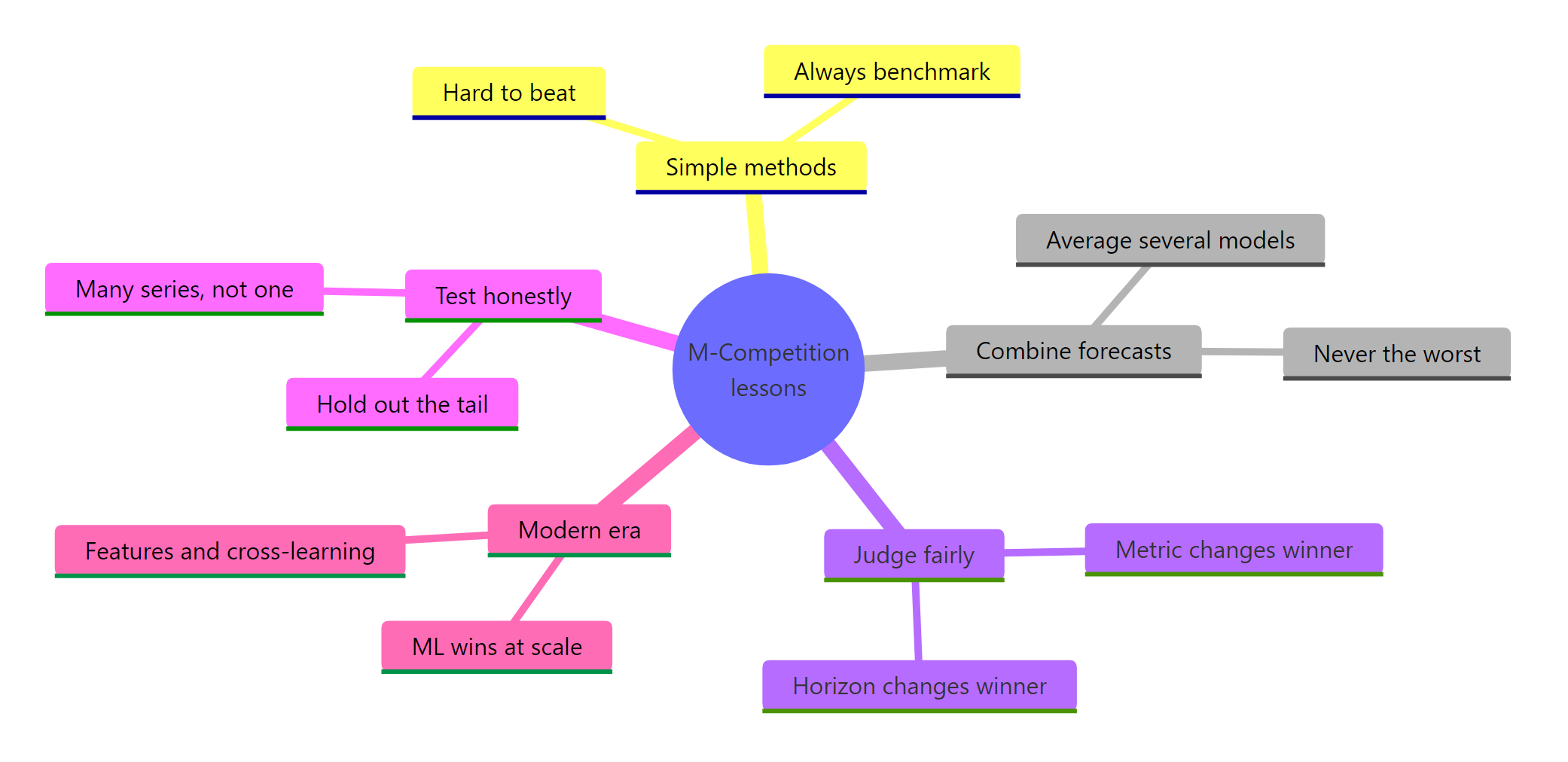
Figure 4: The durable lessons of the M competitions at a glance.
The unifying thread is humility. The M competitions reward forecasters who benchmark against simple methods, combine rather than gamble on one model, judge accuracy on the metric and horizon that matter, and never trust a score on data the model has already seen.
References
- Makridakis, S., Spiliotis, E., & Assimakopoulos, V. (2020). The M4 Competition: 100,000 time series and 61 forecasting methods. International Journal of Forecasting. Link
- Makridakis, S., Spiliotis, E., & Assimakopoulos, V. (2022). M5 accuracy competition: Results, findings, and conclusions. International Journal of Forecasting. Link
- Makridakis, S., & Hibon, M. (2000). The M3-Competition: results, conclusions and implications. International Journal of Forecasting. Link
- Hyndman, R. J., & Athanasopoulos, G. Forecasting: Principles and Practice (3rd ed.). OTexts. Link
- Smyl, S. (2020). A hybrid method of exponential smoothing and recurrent neural networks for time series forecasting (M4 winner). International Journal of Forecasting. Link
- Montero-Manso, P., Athanasopoulos, G., Hyndman, R. J., & Talagala, T. S. (2020). FFORMA: Feature-based forecast model averaging. International Journal of Forecasting. Link
- Hyndman, R. J. forecast package reference (thetaf, ets, accuracy). Link
- feasts and the tidyverts project reference. Link
Continue Learning
- Combining Forecasts in R goes beyond the simple average, showing how to weight and stack forecasts for even better combinations.
- Forecast Accuracy in R covers MASE, sMAPE, and RMSSE in depth, so you can choose the right metric with confidence.
- Time Series Cross-Validation in R replaces our single hold-out with many rolling origins, the fairest way to score a forecasting method.