Intermittent Demand Forecasting in R: Croston and Friends
Intermittent demand is demand that arrives in scattered bursts with many zero periods in between, the pattern you see with spare parts and slow-moving items. Croston's method forecasts it by smoothing two things separately, how big each demand is and how often it arrives, then dividing one by the other to get a steady demand rate. This tutorial builds Croston's method and its two best-known relatives, SBA and TSB, from scratch in R, then checks them against the forecast package.
What makes intermittent demand so hard to forecast?
Picture a warehouse that stocks a replacement gearbox for an old machine. Most months nobody orders one. Then a machine breaks, three orders land in a week, and it goes quiet again for half a year. The demand history is mostly zeros with occasional spikes. Ordinary forecasters were built for series that are always "on", like daily sales of a popular product, so they perform poorly here. Let's create such a series and look at it.
We simulate 48 months of demand for a slow-moving part. Each month a demand either arrives or it does not, and when it does, a small number of units go out. We arrange the result as a 4-year by 12-month grid so the gaps are easy to see.
Each row is one year. Most cells are zero, and the non-zero months carry a handful of units each. Demand clearly clusters: Year 4 is busy, Year 1 is nearly dead. This is the signature of intermittent demand, long stretches of nothing punctuated by bursts.
Now let's put a number on how sparse it is. Two quick summaries tell the story: the share of months with no demand at all, and the average units shipped per month across the whole history.
Almost 69% of the months are zero, yet on average the part still ships about 1.67 units a month. That average is the honest planning target. You cannot order 1.67 gearboxes in a given month, but over a year that rate tells you to keep roughly 20 in stock. A picture makes the burstiness obvious.
The vertical spikes stand alone with wide flat gaps between them. Nothing gradual is happening, so a method that expects a smooth trend has nothing to work with.
Here is why the usual tool struggles. Simple exponential smoothing, or SES, forecasts the next value as a weighted average that leans on recent months. On an always-on series that is sensible. On this series the forecast slides toward zero during every dry spell, then jerks upward right after a sale. Let's watch the one-step-ahead SES forecast and see how far it swings.
Across the series the SES forecast ranges from 0 all the way to 3.31, depending only on how recently a demand happened to land. Read it just after a spike and it says 3; read it after a long gap and it says 0. Neither is the true rate of about 1.67. The number you get depends on timing luck, not on the underlying demand.
Croston's insight is to stop forecasting the raw series and instead forecast two calmer quantities: how big demands are, and how far apart they are. Both are far more stable than the jumpy raw series, and combining them recovers the rate we actually want.
Try it: When this part does sell, how many units typically go out? Compute the average of only the non-zero months of demand. It should come out to about 5.3.
Click to reveal solution
Explanation: demand > 0 is a TRUE/FALSE mask, and demand[demand > 0] keeps only the months that actually shipped. Their average, about 5.33 units, is the "typical order size" that Croston's method will smooth.
How does Croston's method actually work?
Croston's method answers two separate questions and then multiplies them back together. The first question is "when it sells, how much does it sell?" The second is "how many months pass between sales?" Each answer is a slow, well-behaved series that exponential smoothing handles well. The diagram below shows the whole pipeline.
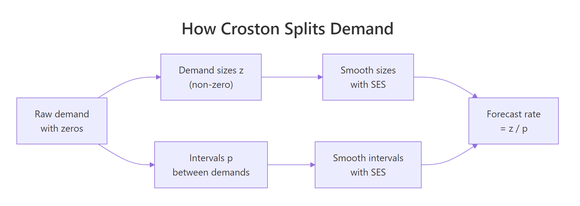
Figure 1: Croston splits one demand series into demand sizes and inter-arrival intervals, smooths each with exponential smoothing, then recombines them into a rate.
Let's do the split by hand. We find the months where demand is non-zero. The demand sizes are just those values. The intervals are the gaps between consecutive non-zero months, measured in months. The first interval is simply the position of the first sale.
The first vector, z, is the size each time the part sold: 5 units, then 4, then 5, with the sizes staying in a narrow range. The second vector, p, is how many months apart those sales were: the first sale came in month 6, the next 3 months later, the next 9 months after that. These two streams are what Croston forecasts, one at a time.
Now we apply exponential smoothing to each stream. Exponential smoothing keeps a running estimate and nudges it toward each new observation by a fraction $\alpha$ (alpha), a number between 0 and 1. After the $i$-th sale the size estimate updates as $\hat{z} \leftarrow \hat{z} + \alpha\,(z_i - \hat{z})$, and the interval estimate updates the same way. A small alpha means slow, steady learning; a large alpha means the estimate reacts fast to the latest sale. If you want the deeper mechanics of that update, see our guide to exponential smoothing in R. The forecast rate is then the smoothed size divided by the smoothed interval:
$$\hat{y} = \frac{\hat{z}}{\hat{p}}$$
Here is the whole method in one function. We seed both estimates with their first observed value, then smooth through the rest.
The function returns three numbers. The smoothed size is 5.227 units, meaning a typical sale is a bit above five units. The smoothed interval is 3.243 months, meaning sales come roughly every three months. Divide the two and you get a forecast of 1.612 units per month, close to the honest average of 1.67 we computed earlier, but built from stable parts instead of the jumpy raw series.
You do not have to hand-roll this every time. The forecast package ships Croston's method as croston(). Let's confirm our from-scratch version agrees with it, which is the best way to know we understood the algorithm.
Identical to our hand-coded 1.612. The h = 6 argument asks for a six-month-ahead forecast, but notice every month gets the same number: Croston produces one flat rate and repeats it. That is expected, since the method estimates a level, not a trend or a season.
croston() returns a rate with no honest way to attach an "80% confidence" band. If you need uncertainty, you build it separately, for example by simulating demand from the fitted size and interval.The smoothing parameter alpha is the one knob you control, so it helps to feel what it does. Let's forecast the same series across a range of alpha values.
A larger alpha leans harder on recent sales, which here were on the busy side, so the forecast climbs from 1.21 at alpha 0.05 up to 2.71 at alpha 0.30. There is no universally correct value. A common default is a small alpha between 0.05 and 0.2, and later we will pick one by testing on held-out data.
Try it: Forecast demand with a more reactive alpha of 0.3 using our croston_fit() function, and read off the rate. It should match the 2.709 from the sweep above.
Click to reveal solution
Explanation: With alpha 0.3 the estimates track the recent busy months closely, pushing the rate up to 2.71. That is why a high alpha is risky on short intermittent histories: one lucky burst raises the forecast.
Why does Croston's forecast run high, and how does SBA fix it?
Croston's method has a subtle flaw that took the field 30 years to pin down. On average, across many series, it forecasts a little too high. The reason is mathematical: Croston forecasts a ratio, smoothed size over smoothed interval, and the average of a ratio is not the ratio of the averages. That gap tilts the estimate upward. In 2005 Syntetos and Boylan proved the size of the bias and gave a clean correction.
Their fix, now called the Syntetos-Boylan Approximation or SBA, simply multiplies Croston's forecast by a shrinkage factor that depends on alpha:
$$\hat{y}_{\text{SBA}} = \left(1 - \frac{\alpha}{2}\right)\frac{\hat{z}}{\hat{p}}$$
Where:
- $\hat{z}/\hat{p}$ is the ordinary Croston rate
- $\alpha$ is the same smoothing parameter Croston uses
- $\left(1 - \frac{\alpha}{2}\right)$ is the correction factor, always a little below 1
Because the factor is below 1, SBA always pulls the forecast down a touch. With alpha 0.1 the factor is 0.95, a 5% trim. Let's code it as a one-line wrapper around our Croston function and compare the two on our series.
SBA nudges the forecast from 1.612 down to 1.531. On this single series that is just a small shift, and you might reasonably ask whether it is worth bothering with. The honest way to answer is not to stare at one series, where luck dominates, but to simulate many series from a known truth and check which method lands closer on average.
Let's generate 3,000 intermittent series, each with a demand probability of 0.3 and an average size of 5, so the true rate is exactly $0.3 \times 5 = 1.5$ units per month. We forecast each series with both methods and average the results.
There it is. Averaged over 3,000 series, Croston's forecast is 1.573 against a truth of 1.5, an upward bias of 0.073. SBA averages 1.494, a bias of just -0.006, more than ten times smaller. The tiny per-series trim adds up to a forecast that is essentially unbiased. If you hold a lot of slow-moving parts, that removed bias is fewer units of chronic over-stock across the whole catalog.
Try it: Compute the SBA correction factor for a smoothing parameter of 0.2. Use the formula one minus alpha over two.
Click to reveal solution
Explanation: At alpha 0.2 the factor is 0.9, a 10% trim. Larger alpha means a bigger correction, because a more reactive Croston estimate carries more of the ratio bias.
What happens when a product becomes obsolete? Meet TSB.
Croston and SBA share a blind spot. They only update their estimates when a demand arrives. During a long run of zeros, nothing changes, so the forecast just sits at its last value forever. That is fine for a part with steady demand, but it is dangerous for a part that is dying. If the last gearbox ever sold was two years ago, Croston still forecasts the old rate, and you keep stock you will never sell.
Teunter, Syntetos and Babai fixed this in 2011 with a method usually called TSB. Instead of tracking the interval between demands, TSB tracks the probability that a demand happens in any given month, and it updates that probability every single period, including the zeros. When demands stop, the probability decays toward zero, and so does the forecast. Two update rules run each month, with their own smoothing parameters:
$$\hat{p}_t = \hat{p}_{t-1} + \beta\,(d_t - \hat{p}_{t-1}) \qquad \hat{z}_t = \hat{z}_{t-1} + \alpha\,(z_t - \hat{z}_{t-1})$$
Where:
- $d_t$ is 1 if a demand occurred this month and 0 otherwise
- $\hat{p}_t$ is the smoothed probability of a demand, updated every month with rate $\beta$ (beta)
- $\hat{z}_t$ is the smoothed demand size, updated with rate $\alpha$ only in months that had a demand
- the forecast is $\hat{p}_t \times \hat{z}_t$, a probability times a size
Let's code it. The probability updates on every iteration; the size updates only when the month was non-zero.
TSB reads our series as a 36% chance of a demand each month, at a typical size of 5.227 units, giving a forecast of 1.883 units per month. It is a bit higher than Croston here because our series stays active to the end. The real advantage shows up when demand dries up. Let's take the same series but zero out the last 18 months, as if the part went obsolete after month 30, and compare the two methods.
After 18 dead months, Croston still forecasts 1.195 units a month, frozen at the value it held when the last sale happened. TSB has more than halved to 0.585 and keeps falling, because its demand probability shrank a little every one of those quiet months. TSB's forecast responded to the drop in demand; Croston's stayed frozen at its last value.
Try it: Run TSB on the obsolete dead series but with a faster-forgetting beta of 0.2 instead of 0.05. A bigger beta should decay the forecast even lower than 0.585.
Click to reveal solution
Explanation: A beta of 0.2 lets the probability fall four times faster than 0.05, so after 18 dead months the forecast has collapsed to 0.032, almost zero. Bigger beta means quicker reaction to obsolescence, at the cost of more jitter while the part is still alive.
Which method should you use? Classify your demand first.
You now have three tools. Rather than guess, the field uses a simple two-number test to sort any demand series into a category, and each category points to a method. The first number is the average inter-demand interval, or ADI, which is how many months pass between demands on average. The second is the squared coefficient of variation of the non-zero sizes, written $CV^2$, which measures how wildly the order sizes swing:
$$\text{ADI} = \frac{\text{number of months}}{\text{number of demands}} \qquad CV^2 = \left(\frac{\sigma_z}{\mu_z}\right)^2$$
Here $\sigma_z$ and $\mu_z$ are the standard deviation and mean of the non-zero demand sizes. Syntetos, Boylan and Croston proposed cutoffs of 1.32 for ADI and 0.49 for $CV^2$, which split the world into four named quadrants.
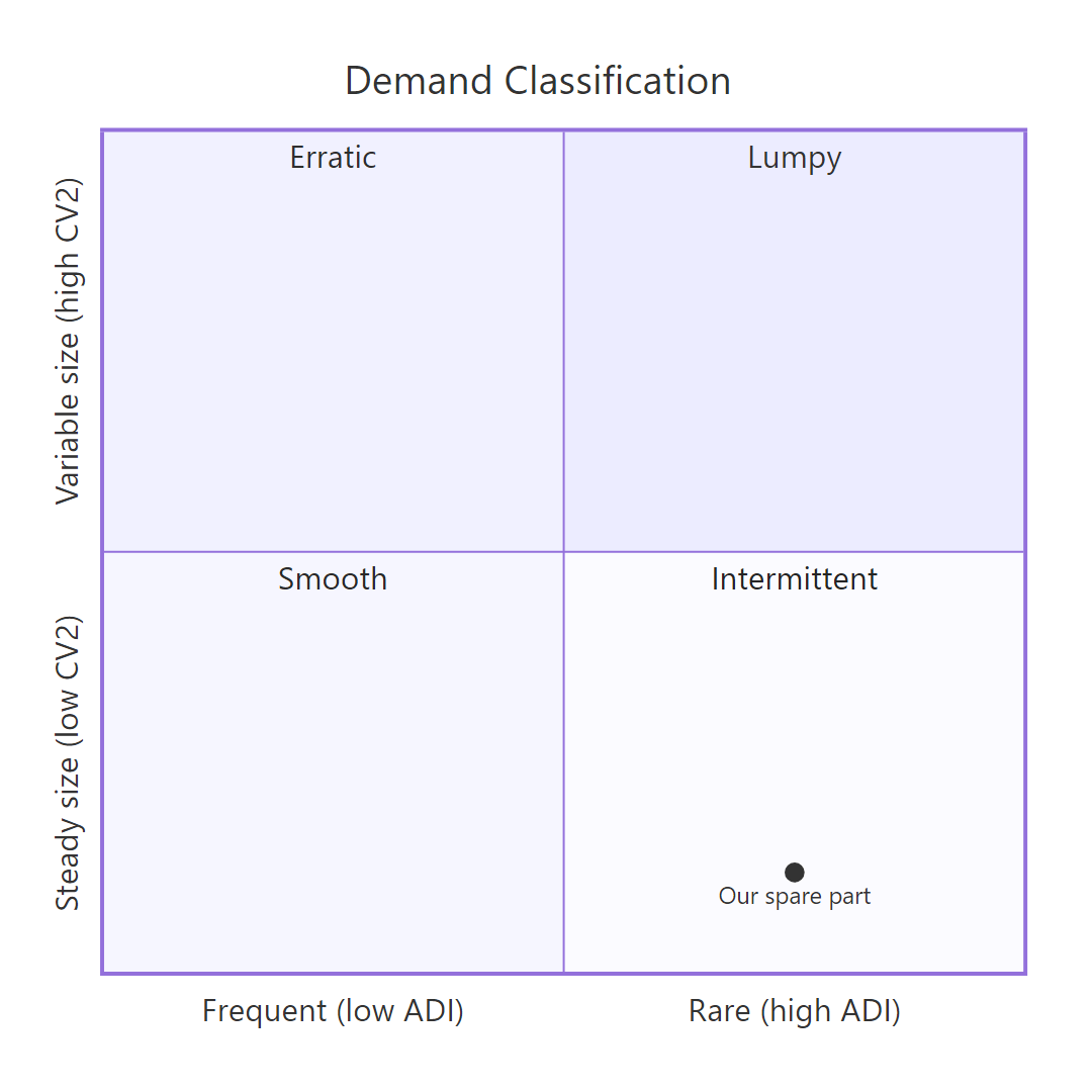
Figure 2: ADI and the squared coefficient of variation sort demand into four classes, each with a recommended forecasting approach.
Let's compute both numbers for our series and read off its class.
Our part has an ADI of 3.2, so demands are rare, roughly one every three months. Its $CV^2$ is only 0.054, so when it does sell the sizes are quite consistent, all in the four-to-eight range. Rare but steady-sized lands it in the intermittent quadrant, the classic home turf of Croston and SBA. This table sums up the four classes and what to reach for.
| Class | ADI | CV² | What it looks like | Method |
|---|---|---|---|---|
| Smooth | Low | Low | Sells most periods, steady size | Regular exponential smoothing |
| Intermittent | High | Low | Rare, but consistent size | Croston or SBA |
| Erratic | Low | High | Frequent, wildly varying size | SBA |
| Lumpy | High | High | Rare and wildly varying | SBA, and expect low accuracy |
Try it: Classify a series that sells every month with a steady size. Run classify_demand() on ex_series below and read the class label. It should come back as "smooth".
Click to reveal solution
Explanation: With a demand every month the ADI is 1, well below 1.32, and the Poisson sizes vary little, so $CV^2$ stays under 0.49. That is the smooth quadrant, where plain exponential smoothing beats Croston, no interval-splitting needed.
How do you measure accuracy when the data is full of zeros?
Scoring intermittent forecasts trips up newcomers, because the most popular error metric breaks down on this data. Mean absolute percentage error, MAPE, divides the error by the actual value. When the actual is zero, and here two of every three months are zero, you are dividing by zero. Let's split our series into a 36-month training set and a 12-month test set, fit Croston on the training months, then try to score the forecast with MAPE.
MAPE returns Inf, infinity, because of the division by zero in the test set. It is useless here, and so is any metric built on percentage errors. You need metrics that survive zeros. Two good ones are the root mean squared error, RMSE, which just squares the raw errors, and the cumulative bias, the total forecast units minus the total actual units over the horizon. Cumulative bias is the one inventory planners care about most, since it is the over- or under-stock that piles up. For a fuller tour of scoring, see forecast accuracy in R. Let's tabulate all four flat forecasts against the same test window.
Every method here under-forecasts, all four cumulative biases are negative, because this particular test window happened to be a busy stretch that the calmer first 36 months did not predict. On this one split TSB looks best and SBA looks worst, the reverse of what the theory promised. That is not a real result, it is the noise of judging a forecast on a single 12-month window. One draw of the dice tells you almost nothing.
The fix is to average over many series, exactly as we did for the bias. Let's simulate 3,000 series from the same known truth of 1.5 and measure each method's mean absolute error against that truth.
Over 3,000 series SBA has the lowest average error, 0.295, beating both Croston at 0.315 and TSB at 0.331. This is the same verdict the bias experiment gave, and it is the one to trust: SBA is the safe default for stable intermittent demand, with TSB reserved for products at risk of dying out.
Try it: Write a tiny cumulative-bias helper that takes a flat forecast and the actual test vector, and returns total forecast minus total actual. Test it with a forecast of 1.5 against test. It should return -14.
Click to reveal solution
Explanation: A flat forecast of 1.5 over 12 months predicts 18 units, but the test window actually shipped 32, so the cumulative bias is 18 minus 32, a shortfall of 14 units. Negative means you would have under-stocked.
The complete workflow, end to end
Putting the pieces together, a sound intermittent-demand routine is: classify the series, let the class choose the method, forecast the rate, and sanity-check it against the plain average. All the functions we built earlier combine into one short block.
The routine classifies the part as intermittent, which selects SBA, giving a forecast of 1.531 units per month. That the rate sits just below the raw sample mean of 1.667 is a good sign, it is the deliberate SBA bias correction at work, not a mistake. This four-line pattern scales to a whole catalog: loop it over every part number and you have a defensible, method-matched forecast for each.
Practice Exercises
These combine several ideas from the tutorial. Try each before opening the solution. The functions croston_fit(), sba_fit(), tsb_fit(), and classify_demand() from above are available.
Exercise 1: A one-call multi-method forecaster
Write a function forecast_all() that takes a demand series and returns a named vector with the Croston, SBA, and TSB forecasts, so you can compare all three at a glance. Run it on demand.
Click to reveal solution
Explanation: Wrapping the three calls in one function gives a compact dashboard. SBA sits just under Croston, as its correction factor guarantees, while TSB reads higher here because the series stays active to the end.
Exercise 2: Auto-select the method from the class
Write recommend() that classifies a series and returns both its class and the method you should use: SBA for intermittent or lumpy demand, Croston otherwise. Run it on demand.
Click to reveal solution
Explanation: The rule encodes the recommendation table: the two hardest quadrants, intermittent and lumpy, both route to SBA, while smoother patterns fall back to plain Croston. Drop this into a catalog loop for automatic method selection.
Exercise 3: Tune alpha by rolling evaluation
Write alpha_grid() that searches a grid of alpha values for Croston, trains on the first 70% of a series, forecasts the last 30%, and returns the alpha with the smallest mean absolute error. Run it on demand.
Click to reveal solution
Explanation: The search picks the smallest alpha, 0.05, because our test window is quieter than the busy training tail, so the most conservative, slowest-reacting forecast scores best. On a real catalog you would run this per part and cap the grid at a sensible maximum like 0.3.
Summary
Intermittent demand, all those zeros with occasional spikes, defeats ordinary forecasters, but a small family of purpose-built methods handles it cleanly. The trick they share is to stop forecasting the raw series and instead forecast demand size and demand timing separately.
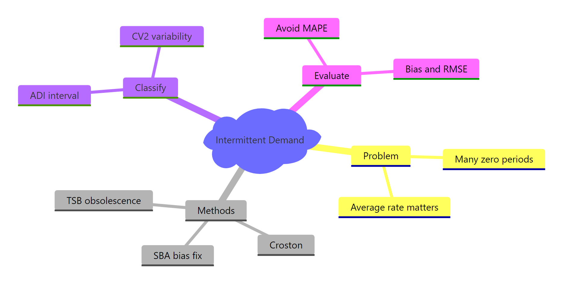
Figure 3: The intermittent-demand toolkit at a glance, from the problem to the three methods to how you evaluate them.
| Method | What it smooths | Best for | One-line reason |
|---|---|---|---|
| Croston | Size and interval, on demand months | Stable intermittent demand | Splits size from timing, but runs slightly high |
| SBA | Croston, times (1 - alpha/2) | Most intermittent and lumpy demand | Removes Croston's upward bias, the safe default |
| TSB | Size, plus demand probability every month | Products at risk of obsolescence | Decays toward zero when demand stops |
Key takeaways:
- Forecast the demand rate, size divided by interval, not the jumpy raw series.
- Croston splits the series into sizes and intervals and smooths each; the forecast package's
croston()reproduces it exactly. - SBA trims Croston by a factor just below one and is nearly unbiased, making it the default for intermittent and lumpy parts.
- TSB updates a demand probability every period, so it alone reacts when a product goes obsolete.
- Classify first with ADI and $CV^2$, and never use MAPE, score with bias and scaled error over many series.
Frequently Asked Questions
Can I use Croston's method for demand that is not intermittent?
You can, but you usually should not. On smooth demand that sells most periods, plain exponential smoothing or an ETS model is more accurate, because splitting the series into sizes and intervals only helps when there are real gaps to model. Run the ADI and CV² classification first: if the series lands in the smooth quadrant, forecast it the normal way.
How do I choose the smoothing parameter alpha?
Start with a small value between 0.05 and 0.2, which keeps the estimate stable on short, noisy histories. If you want to tune it, hold out the most recent months, forecast them across a grid of alpha values, and keep the one with the lowest mean absolute error, exactly what Exercise 3 above does. Avoid large alpha on short series, since one busy stretch can drag the forecast up.
What is the real difference between SBA and TSB?
SBA is Croston with a small downward correction that removes its upward bias; it still only updates when a demand arrives. TSB instead tracks the probability of a demand and updates it every month, so its forecast decays toward zero when demand stops. Use SBA as your default for active parts, and switch to TSB when a product might be going obsolete.
Why does Croston give the same forecast for every future month?
Croston estimates a level, the average demand rate, not a trend or a seasonal pattern. With nothing to trend toward, the best flat estimate of next month is also the best estimate of the month after, so croston() repeats one number across the whole horizon. That flat rate is what you feed into stock and reorder calculations.
Which R package should I use in production?
For a single Croston forecast, the forecast package's croston() is enough. For SBA, TSB, automatic parameter optimization, and demand classification in one place, use the tsintermittent package (crost, tsb, idclass) or the smooth package. The hand-coded versions in this tutorial match what those packages compute, so you can adopt them knowing what runs under the hood.
References
- Hyndman, R. J., forecast::croston() reference, the canonical R implementation of Croston's method. Link
- Shenstone, L. and Hyndman, R. J., Stochastic models underlying Croston's method for intermittent demand forecasting. Journal of Forecasting (2005). Link
- Syntetos, A. A. and Boylan, J. E., The accuracy of intermittent demand estimates. International Journal of Forecasting (2005), the paper that introduced SBA. Link
- Teunter, R. H., Syntetos, A. A. and Babai, M. Z., Intermittent demand: Linking forecasting to inventory obsolescence. European Journal of Operational Research (2011), the TSB method. Link
- Kourentzes, N., tsintermittent::crost() reference, a production R package implementing Croston, SBA and TSB. Link
- tsintermittent: Intermittent Time Series Forecasting, CRAN package page. Link
- Hyndman, R. J. and Athanasopoulos, G., Forecasting: Principles and Practice, section on count and intermittent time series. Link
Continue Learning
- Exponential Smoothing in R, the SES engine that sits inside every method in this tutorial, explained from first principles.
- Forecast Accuracy in R, a deeper look at error metrics, including the scaled errors that replace MAPE on intermittent data.
- Backtesting Forecasts in R, how to evaluate a forecast honestly with rolling origins instead of a single lucky hold-out.