Count Time Series in R: INGARCH with tscount
A count time series is a sequence of whole-number counts recorded over time, like weekly disease cases or daily support tickets. INGARCH models, fit in R with the tscount package, forecast these integer counts while respecting a fact that ordinary ARIMA ignores: a count can never be negative or fractional.
This tutorial builds up from the raw data to a working forecast. The exploration uses base R and runs right here in your browser. The modeling uses the tscount package, which you run in a local R session, and every result you see below was produced by actually running that code.
What makes a count time series different from an ordinary time series?
Most forecasting tutorials assume your data is continuous: temperatures, stock prices, sales in dollars. Counts are different. They are whole numbers that stop at zero, they are often small, and their spread tends to grow as their level grows. Feed counts into a method built for continuous, bell-shaped data and it will hand you a forecast of 11.54 cases, or even a negative one.
Let's make this concrete with a real dataset. The campy data records the number of Campylobacter infections reported every four weeks in a region of Quebec, 140 observations in all. We will paste the counts in directly so you can explore them immediately.
The plot shows exactly the features that make counts awkward. Every value is a whole number. Many are small (the minimum is 1). There is a yearly rise and fall. And around observation 100 there is a sharp outbreak that peaks at 55 cases, far above the usual level.
That last point hints at the deepest issue. For continuous data we often assume the spread is roughly constant. For counts, the spread grows with the level. A helpful first check is to compare the mean with the variance.
Here is why that ratio matters. The Poisson distribution, the natural starting point for counts, assumes the variance equals the mean. Our variance is 4.6 times the mean. When the variance is bigger than the mean, statisticians call it overdispersion, and it is the rule rather than the exception for real count data. Any honest count model has to allow for it.
Now let's see what a standard tool does with this series. We will let auto.arima pick an ARIMA model and forecast three steps ahead.
The forecasts are 11.54, 12.80, and 13.43. You cannot observe 11.54 infections; counts are whole numbers. And because ARIMA builds symmetric, bell-shaped intervals, a series with smaller counts would get an interval that dips below zero, predicting a negative number of cases. ARIMA simply does not know that counts stop at zero and come in whole units.
Try it: Overdispersion should show up in different stretches of the series, not just overall. Compute the variance-to-mean ratio separately for the first 70 observations and the last 70, and check that both are clearly above 1.
Click to reveal solution
Explanation: Both halves are overdispersed (ratio above 1), and the second half, which contains the big outbreak, is far more overdispersed than the first. Overdispersion is a property of the whole series, so the model must handle it everywhere.
What is the INGARCH model, and how does it actually work?
The trick behind INGARCH is to stop modeling the counts directly and instead model their conditional mean, the expected count at each time step given everything that came before. Call that expected count $\lambda_t$. At every step the model draws the actual count from a count distribution (Poisson to start) whose mean is $\lambda_t$, so the counts are always whole numbers by construction.
The clever part is how $\lambda_t$ moves over time. It responds to two things. First, the most recent count: if you just saw a spike, your expectation for right now should rise. Second, the most recent expectation itself: the level has momentum and carries forward smoothly. Think of a thermostat with memory. It reacts to the last reading, but it also remembers where it was aiming a moment ago.

Figure 1: How INGARCH turns the recent count and recent mean into the next count.
Those two feedback channels give the model its name. It is the count-data cousin of the GARCH models used for financial volatility, so it is called the integer-valued GARCH, or INGARCH, model. The simplest useful version uses one lag of each channel, written INGARCH(1,1).
If you like equations, here is the INGARCH(1,1) model in full. If not, the simulation just below teaches the same thing in code, so feel free to skip ahead.
$$Y_t \mid \mathcal{F}_{t-1} \sim \text{Poisson}(\lambda_t), \qquad \lambda_t = \beta_0 + \beta_1 Y_{t-1} + \alpha_1 \lambda_{t-1}$$
Where:
- $Y_t$ = the count at time $t$
- $\mathcal{F}_{t-1}$ = the history, everything known up to time $t-1$
- $\lambda_t$ = the conditional mean, the expected count right now
- $\beta_0$ = a baseline level (the intercept)
- $\beta_1$ = how strongly the most recent count pushes the mean up (reactivity)
- $\alpha_1$ = how strongly the previous mean carries forward (memory)
The best way to believe this is to build it yourself. The loop below starts with a level, then at each step computes $\lambda_t$ from the last count and last mean, and draws a Poisson count. This is the entire mechanism in a few lines.
Look at what happened. We never told the series to hover around any particular value, yet it settled into a stable band with an average near 5.6. That stable level is not an accident. It is set by the coefficients: a bigger $\beta_0$ lifts the whole series, while $\beta_1$ and $\alpha_1$ control how much recent history pulls each new value. Every count is a whole number because it came out of rpois, exactly as a real count series would.
Try it: The two feedback strengths add up to $\beta_1 + \alpha_1 = 0.7$ in the simulation above. Rerun it with alpha1 = 0.6 so they add up to 1, and watch what happens to the average count.
Click to reveal solution
Explanation: With the two coefficients summing to exactly 1, the series loses its anchor and drifts upward without bound, so the average explodes from about 5.6 to 182.5. That is the boundary of stability, and it is the reason well-behaved INGARCH models keep the feedback coefficients adding up to less than 1. We will meet this rule again in the next section.
How do you fit an INGARCH model in R with tscount?
You do not need to write the loop yourself. The tscount package fits INGARCH models by maximum likelihood with a single function, tsglm(). Because it is a specialized package, the modeling code in this section and the ones that follow runs in a local R session rather than in your browser. Every output shown is the real result of running that code.
install.packages("tscount") once in your R session. The package provides the campy dataset used here, so you can reproduce every result exactly.Let's fit the INGARCH(1,1) Poisson model from the previous section to the real data. The model argument is where you specify the two feedback channels: past_obs is the lag on past counts (the $\beta$ terms) and past_mean is the lag on past means (the $\alpha$ terms).
# Run this in a local R session (needs the tscount package)
library(tscount)
data(campy)

pois11 <- tsglm(campy, model = list(past_obs = 1, past_mean = 1), distr = "poisson")
summary(pois11)
#>
#> Call:
#> tsglm(ts = campy, model = list(past_obs = 1, past_mean = 1),
#>     distr = "poisson")
#>
#> Coefficients:
#>              Estimate  Std.Error  CI(lower)  CI(upper)
#> (Intercept)     2.389     0.6162      1.181      3.597
#> beta_1          0.518     0.0595      0.402      0.635
#> alpha_1         0.269     0.0853      0.102      0.436
#> Standard errors and confidence intervals (level =  95 %) obtained
#> by normal approximation.
#>
#> Link function: identity
#> Distribution family: poisson
#> Number of coefficients: 3
#> Log-likelihood: -436.7283
#> AIC: 879.4566
#> BIC: 888.2815
#> QIC: 879.7023
Read the coefficients like the pieces of the recursion you just simulated. The (Intercept) of 2.389 is the baseline $\beta_0$. The beta_1 of 0.518 is the reactivity: a little over half of a surprise in the latest count feeds into the next expected count. The alpha_1 of 0.269 is the memory: about a quarter of the previous expectation carries forward. Both confidence intervals exclude zero, so both channels earn their place.
Notice that the link function is identity. That means $\lambda_t$ is built by plain addition, exactly as in the formula, which keeps the coefficients easy to read. There is also a log link, which we will meet shortly, for when you need covariates or a multiplicative structure.
Try it: Fit the same INGARCH(1,1) model but with link = "log" instead of the default identity link, using the negative binomial distribution, and read off its AIC.
# Run locally. Change the link argument, then read the AIC.
logfit <- tsglm(campy, model = list(past_obs = 1, past_mean = 1),
                link = "identity", distr = "nbinom")   # change "identity" to "log"
AIC(logfit)
# Expected: an AIC near 820
Click to reveal solution
logfit <- tsglm(campy, model = list(past_obs = 1, past_mean = 1),
                link = "log", distr = "nbinom")
round(AIC(logfit), 2)
#> [1] 820.5
Explanation: The log link models the logarithm of the conditional mean, so the feedback becomes multiplicative. Its AIC of 820.5 is almost identical to the identity-link version we build next, so for this series the choice of link barely matters. The log link earns its keep when you add covariates that can push the mean in either direction.
How do you pick the distribution and model order?
Two decisions turn the basic INGARCH into a model that fits your data: which conditional distribution to use, and how many lags to include. The good news is that both decisions are guided by numbers you already know how to read.
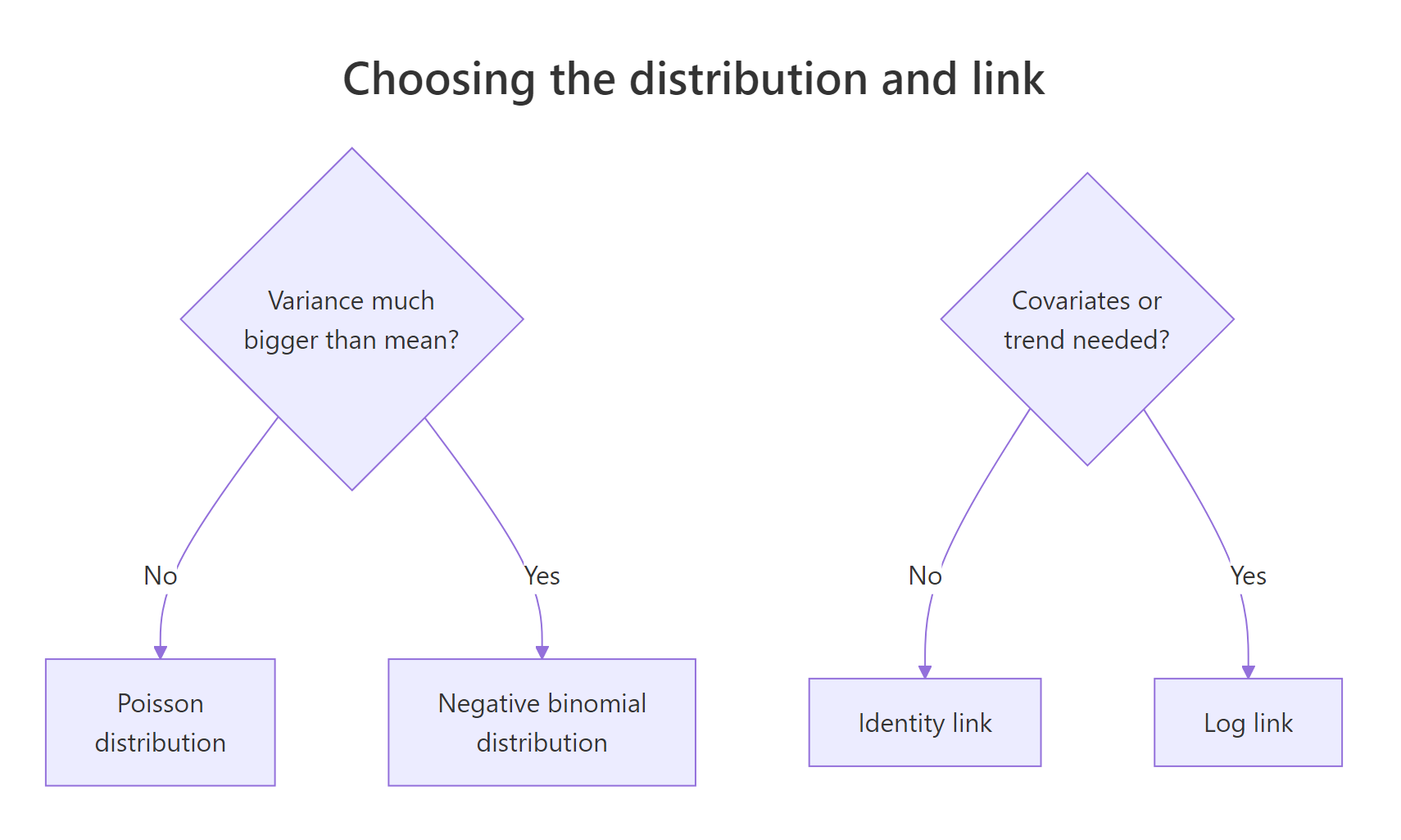
Figure 2: Picking the conditional distribution and link function.
Start with the distribution. We saw that campy is heavily overdispersed: its variance is 4.6 times its mean. The Poisson distribution cannot represent that, because it forces the variance to equal the mean. The negative binomial distribution adds one extra parameter that lets the variance exceed the mean, so it is the right choice for overdispersed counts. Let's refit with it.
nbin11 <- tsglm(campy, model = list(past_obs = 1, past_mean = 1), distr = "nbinom")
summary(nbin11)
#>
#> Call:
#> tsglm(ts = campy, model = list(past_obs = 1, past_mean = 1),
#>     distr = "nbinom")
#>
#> Coefficients:
#>              Estimate  Std.Error  CI(lower)  CI(upper)
#> (Intercept)     2.389      0.969     0.4895      4.289
#> beta_1          0.518      0.101     0.3200      0.717
#> alpha_1         0.269      0.139    -0.0029      0.542
#> sigmasq         0.109         NA         NA         NA
#> Standard errors and confidence intervals (level =  95 %) obtained
#> by normal approximation.
#>
#> Link function: identity
#> Distribution family: nbinom (with overdispersion coefficient 'sigmasq')
#> Number of coefficients: 4
#> Log-likelihood: -406.4186
#> AIC: 820.8371
#> BIC: 832.6037
#> QIC: 889.7003
The mean coefficients barely move, which is reassuring: the story about reactivity and memory is unchanged. What is new is sigmasq, the overdispersion parameter that quantifies the extra spread. And notice the log-likelihood jumped from -436.7 to -406.4. That is a large improvement from a single extra parameter.
To compare models properly we use the AIC and BIC, two scores that reward fit but penalize extra parameters, so lower is better. While we are at it, we will add a seasonal model. The campy counts rise and fall once a year, and the data is recorded 13 times a year, so a feedback term at lag 13 lets last year's level inform this year's. We add it with past_mean = 13.
seas <- tsglm(campy, model = list(past_obs = 1, past_mean = 13), distr = "nbinom")

comparison <- data.frame(
  model = c("Poisson (1,1)", "NegBin (1,1)", "NegBin seasonal"),
  AIC = round(c(AIC(pois11), AIC(nbin11), AIC(seas)), 1),
  BIC = round(c(BIC(pois11), BIC(nbin11), BIC(seas)), 1))
print(comparison, row.names = FALSE)
#>            model   AIC   BIC
#>    Poisson (1,1) 879.5 888.3
#>     NegBin (1,1) 820.8 832.6
#>  NegBin seasonal 820.1 831.8
The table tells a clear story. Switching from Poisson to negative binomial drops the AIC by nearly 60 points, a decisive win driven entirely by handling overdispersion. Adding the seasonal lag helps a little more. The negative binomial matters far more than the exact lag structure here, which is typical: get the distribution right first, then fine-tune the lags.
Try it: Maybe the count from two periods ago also helps. Fit a negative binomial model that regresses on both the first and second lags of past counts, using past_obs = c(1, 2), and compare its AIC with the 820.8 of the plain (1,1) model.
# Run locally. Fill in past_obs with the two lags, then read the AIC.
ex_fit <- tsglm(campy, model = list(past_obs = 1, past_mean = 1), distr = "nbinom")
AIC(ex_fit)
# Expected: compare against 820.8
Click to reveal solution
ex_fit <- tsglm(campy, model = list(past_obs = c(1, 2), past_mean = 1), distr = "nbinom")
round(AIC(ex_fit), 2)
#> [1] 823.05
Explanation: The AIC rises from 820.8 to 823.05, so the second lag makes the model worse once you account for the extra parameter. More lags are not automatically better; the AIC keeps you honest by charging for every coefficient you add.
How do you check whether the model fits the data well?
A model that fits the training data is not the same as a model that captures the real structure. Before you trust a forecast, you check three things: whether the residuals still contain patterns, whether competing models score better, and whether the predicted probabilities are honest.
Start with the residuals. A Pearson residual is each observed count minus the count the model expected, divided by the model's standard deviation at that step, so the values are on a comparable scale. If the model has captured the dependence in the series, these leftover residuals should look like noise, with no autocorrelation. We check with the autocorrelation function.
acf(residuals(seas, type = "pearson"), plot = FALSE, lag.max = 13)
#>
#> Autocorrelations of series 'residuals(seas, type = "pearson")', by lag
#>
#> 0.0000 0.0769 0.1538 0.2308 0.3077 0.3846 0.4615 0.5385 0.6154 0.6923 0.7692
#>  1.000 -0.021  0.024  0.058  0.103  0.067 -0.084  0.181  0.014  0.059  0.012
#> 0.8462 0.9231 1.0000
#>  0.117  0.198  0.193
Ignore the value at lag 0, which is always 1. The rest are mostly small, which is what we want: the model has soaked up the strong autocorrelation we saw in the raw series. A couple of values near lag 12 and 13 are a little larger (0.198 and 0.193), a gentle hint that some yearly structure remains, but nothing alarming.
Next, compare models with proper scoring rules. A scoring rule grades the whole predictive distribution, not just the point forecast, and lower scores are better. The scoring() function reports several at once; we will look at three.
scores <- rbind(Poisson = scoring(pois11),
                NegBin = scoring(nbin11),
                Seasonal = scoring(seas))
round(scores[, c("logarithmic", "quadratic", "rankprob")], 3)
#>          logarithmic quadratic rankprob
#> Poisson        3.119    -0.067    2.719
#> NegBin         2.903    -0.070    2.667
#> Seasonal       2.900    -0.071    2.649
The negative binomial models beat the Poisson on every score, and the seasonal model edges ahead on the ranked probability score. This agrees with the AIC table, which is exactly the confirmation you want: two independent yardsticks pointing the same way.
The final check is calibration. A forecast is calibrated if events it calls "20 percent likely" actually happen about 20 percent of the time. The probability integral transform (PIT) histogram tests this. If the model is well calibrated, the bars are flat and even; a U-shape or a hump signals trouble. It produces a plot rather than printed numbers, so run it locally and read the shape.
pit(seas)
# A roughly flat, uniform histogram means the model is well calibrated.Try it: The eye can miss residual autocorrelation. Run a Box-Ljung test on the Pearson residuals of the seasonal model at lag 13 to test formally whether any autocorrelation remains.
# Run locally. Fill in the residual type and the lag.
Box.test(residuals(seas, type = "pearson"), lag = 1, type = "Ljung-Box")
# Expected: a p-value you can compare against 0.05
Click to reveal solution
Box.test(residuals(seas, type = "pearson"), lag = 13, type = "Ljung-Box")
#>
#> 	Box-Ljung test
#>
#> data:  residuals(seas, type = "pearson")
#> X-squared = 23.345, df = 13, p-value = 0.03771
Explanation: The p-value of 0.038 is just below 0.05, so there is mild evidence of leftover autocorrelation, consistent with the small spikes we saw near lag 12 and 13. The model is good but not perfect; a more elaborate seasonal structure could squeeze out the rest.
How do you forecast future counts with prediction intervals?
The whole point of a count model is to predict future counts, and to say how uncertain those predictions are. The predict() function does both. You give it the number of steps ahead with n.ahead, the confidence level with level, and a crucial switch, global = TRUE, which builds the prediction intervals by simulation instead of a normal approximation.
That switch matters. For counts, especially small or skewed ones, the normal approximation gives intervals that are symmetric and can slip below zero. Setting global = TRUE runs a parametric bootstrap that respects the count distribution, so the intervals are made of whole numbers and can be asymmetric. The B argument sets how many bootstrap paths to draw.
set.seed(2024)
fc6 <- predict(seas, n.ahead = 6, level = 0.9, global = TRUE, B = 2000)

round(fc6$pred, 2)
#> Time Series:
#> Start = c(2000, 11)
#> End = c(2001, 3)
#> Frequency = 13
#> [1] 10.51 12.30 11.92 11.65 11.40 11.46

fc6$interval
#> Time Series:
#> Start = c(2000, 11)
#> End = c(2001, 3)
#> Frequency = 13
#>          lower upper
#> 2000.769     2    25
#> 2000.846     2    32
#> 2000.923     2    32
#> 2001.000     2    34
#> 2001.077     1    33
#> 2001.154     2    33
The point forecasts settle toward the series average of about 11 or 12 cases, which is what a stable model should do as it looks further ahead. The intervals are the real payoff. They are made of whole numbers, they are wide (a 90 percent interval of 2 to 25 for the next period), and they are asymmetric, stretching further above the point forecast than below. That asymmetry is honest: an outbreak can push counts far up, but they can never fall below zero.
Try it: Forecasts are often needed just one step ahead. Produce a one-step-ahead forecast from the seasonal model with an 80 percent prediction interval.
# Run locally. Set n.ahead and level for a one-step 80% interval.
set.seed(1)
p1 <- predict(seas, n.ahead = 6, level = 0.9, global = TRUE, B = 2000)
p1$interval
# Expected: a single row with an 80% interval
Click to reveal solution
set.seed(1)
p1 <- predict(seas, n.ahead = 1, level = 0.8, global = TRUE, B = 2000)
round(p1$pred, 2)
#> [1] 10.51
p1$interval
#>          lower upper
#> 2000.769     5    17
Explanation: The one-step point forecast is 10.51 cases, with an 80 percent interval of 5 to 17. The interval is tighter than the 90 percent one above, both because we look only one step ahead and because 80 percent asks for less coverage than 90 percent.
Complete Example: A full count time series workflow
Here is the entire pipeline in one place: explore, fit the best model, confirm it with a score, and forecast. Run it top to bottom in a local R session and you have a working count forecaster.
# tscount and campy are already loaded from earlier in the session

# 1. Explore: counts are overdispersed (variance far exceeds the mean)
round(c(mean = mean(campy), variance = var(campy)), 2)
#>     mean variance
#>    11.54    53.24

# 2. Fit: negative binomial INGARCH with a seasonal lag
fit <- tsglm(campy, model = list(past_obs = 1, past_mean = 13), distr = "nbinom")

# 3. Confirm: the logarithmic score (lower is better)
round(scoring(fit)["logarithmic"], 3)
#> logarithmic
#>         2.9

# 4. Forecast: three periods ahead with a count-aware 90% interval
set.seed(7)
fc <- predict(fit, n.ahead = 3, level = 0.9, global = TRUE, B = 2000)
round(fc$pred, 2)
#> [1] 10.51 12.30 11.92
fc$interval
#>          lower upper
#> 2000.769     2    23
#> 2000.846     3    28
#> 2000.923     3    29
That is the complete recipe. Explore to see that counts are overdispersed, fit a negative binomial INGARCH with any seasonal lag the data calls for, confirm the fit with a score and the diagnostics from the previous section, then forecast with global = TRUE so the intervals respect the count nature of the data.
Practice Exercises
These exercises combine the ideas above. Each uses distinct variable names so your work will not overwrite the models from the tutorial. Every one runs in a local R session with tscount and campy loaded.
Exercise 1: Does a second observation lag pay off?
Fit two negative binomial models to campy: the plain INGARCH(1,1), and one that adds a second lag of past counts with past_obs = c(1, 2). Compare them on both AIC and the logarithmic score, and decide which wins.
# Hint: fit m11 and m21, then build a small data.frame of AIC and
# scoring(...)["logarithmic"] for each.

# Write your code below:
Click to reveal solution
m11 <- tsglm(campy, model = list(past_obs = 1,      past_mean = 1), distr = "nbinom")
m21 <- tsglm(campy, model = list(past_obs = c(1, 2), past_mean = 1), distr = "nbinom")

data.frame(
  model = c("(1,1)", "(2,1)"),
  AIC = round(c(AIC(m11), AIC(m21)), 2),
  logscore = round(c(scoring(m11)["logarithmic"], scoring(m21)["logarithmic"]), 3))
#>   model    AIC logscore
#> 1 (1,1) 820.84    2.903
#> 2 (2,1) 823.05    2.904
Explanation: The simpler (1,1) model wins on both yardsticks: lower AIC and a marginally lower logarithmic score. The extra lag adds complexity without improving prediction, so you keep the smaller model.
Exercise 2: Find the best seasonal feedback lag
You suspect a seasonal feedback term helps, but you are not sure which lag. Write a loop that fits a negative binomial INGARCH with past_obs = 1 and a single past_mean lag of 1, 7, and 13, printing the AIC for each so you can pick the best.
# Hint: loop over the candidate lags with for (L in c(1, 7, 13)) { ... }
# and print AIC(fit) inside the loop.

# Write your code below:
Click to reveal solution
for (L in c(1, 7, 13)) {
  fit <- tsglm(campy, model = list(past_obs = 1, past_mean = L), distr = "nbinom")
  cat(sprintf("past_mean lag %2d -> AIC %.2f\n", L, AIC(fit)))
}
#> past_mean lag  1 -> AIC 820.84
#> past_mean lag  7 -> AIC 822.99
#> past_mean lag 13 -> AIC 820.07
Explanation: The lag-13 model gives the lowest AIC (820.07), the seasonal lag we chose in the tutorial, while lag 7 is actually worse than no seasonal term at all. Looping over candidate lags and comparing AIC is exactly how you search for the right seasonal structure, and here it confirms that last year's level (lag 13) carries the most useful signal.
Exercise 3: Simulate a process, then recover its parameters
This is the ultimate test of understanding. Use the hand-coded recursion from Section 2 to simulate 500 counts from an INGARCH(1,1) process with a known intercept of 2, a beta1 of 0.4, and an alpha1 of 0.3. Then fit a Poisson INGARCH(1,1) with tsglm() and check how close the estimated coefficients come to the truth.
# Hint: build the series with a for loop (as in Section 2), then
# fit tsglm(y, model = list(past_obs = 1, past_mean = 1), distr = "poisson")
# and read coef(). Use set.seed(2025) for a reproducible series.

# Write your code below:
Click to reveal solution
set.seed(2025)
n <- 500
lam <- numeric(n); yy <- numeric(n)
lam[1] <- 6; yy[1] <- rpois(1, lam[1])
b0 <- 2; b1 <- 0.4; a1 <- 0.3
for (t in 2:n) {
  lam[t] <- b0 + b1 * yy[t - 1] + a1 * lam[t - 1]
  yy[t] <- rpois(1, lam[t])
}

rec <- tsglm(yy, model = list(past_obs = 1, past_mean = 1), distr = "poisson")
round(coef(rec), 3)
#> (Intercept)      beta_1     alpha_1
#>       1.836       0.371       0.355
Explanation: The estimates (1.836, 0.371, 0.355) land close to the true values (2, 0.4, 0.3). They are not exact because 500 observations carry only so much information, but they recover the right story: a moderate baseline, and reactivity a bit stronger than memory. Recovering known parameters from simulated data is the standard way to trust that an estimator, and your understanding of it, actually works.
Frequently Asked Questions
When should I use a Poisson INGARCH instead of a negative binomial one?
Use the Poisson version only when the variance of your counts is close to their mean, a situation called equidispersion. The moment the variance is clearly larger than the mean, which is common, switch to the negative binomial version. It adds one overdispersion parameter that lets the spread exceed the mean, and as we saw it dropped the AIC by nearly 60 points on the campy data.
What is the difference between INGARCH and INAR models?
Both model integer counts over time, but through different mechanisms. INGARCH is observation-driven: it updates a conditional mean with a GARCH-like recursion on past counts and past means, which makes feedback and covariates easy to add. INAR (integer autoregressive) models instead use "thinning" operators, where each past count survives into the present with some probability. The tscount package fits the INGARCH family.
Can INGARCH models handle zeros and very low counts?
Yes. Because each count is drawn from a Poisson or negative binomial distribution, zeros arise naturally and no forecast can go negative. If your series is mostly zeros, however, with only occasional demand, a dedicated intermittent-demand method like Croston can be a better fit than a standard INGARCH model.
Can I include external predictors in the model?
Yes. tsglm() accepts an xreg argument for external regressors such as a holiday indicator or a temperature series. With the log link the covariate effects are multiplicative and can push the mean up or down, which is the main reason to prefer the log link over the identity link.
How much data do I need to fit an INGARCH model?
There is no hard rule, but you need enough observations to estimate the coefficients reliably, and a seasonal feedback term needs several full cycles to be trustworthy. The campy series has 140 four-week observations spanning about a decade, which comfortably supports the lag-13 seasonal term we used.
Summary
Count time series need models built for whole, non-negative numbers. INGARCH models, fit with tscount, give you exactly that: a conditional mean that reacts to recent counts and remembers its own level, wrapped in a Poisson or negative binomial distribution so every forecast is a genuine count.

Figure 3: The end-to-end count time series workflow.
| Step | What to do | Key tool |
|---|---|---|
| Explore | Plot the counts; compare variance to mean | plot(), var(), mean() |
| Choose distribution | Poisson if variance is close to the mean, negative binomial if it is much larger | distr = "poisson" or "nbinom" |
| Fit | Set feedback lags in the model list | tsglm(model = list(past_obs, past_mean)) |
| Compare | Rank models; lower is better | AIC(), BIC(), scoring() |
| Diagnose | Residual ACF and PIT calibration | acf(), pit(), Box.test() |
| Forecast | Bootstrap intervals that respect counts | predict(global = TRUE) |
The habits that matter most: check for overdispersion before you pick a distribution, let AIC and the scoring rules choose between models rather than guessing, and always forecast with global = TRUE so your intervals stay in the land of real counts.
References
- Liboschik, T., Fokianos, K., and Fried, R. (2017). tscount: An R Package for Analysis of Count Time Series Following Generalized Linear Models. Journal of Statistical Software, 82(5). Link
- tscount package vignette. Introduction to tsglm and related functions. Link
- tscount reference manual. CRAN. Link
- tscount package page. CRAN. Link
- tsglm function reference. rdrr.io. Link
- A class of count time series models uniting compound Poisson INAR and INGARCH models. arXiv preprint arXiv:2204.12449 (2022). Link
- Hyndman, R.J., and Athanasopoulos, G. Forecasting: Principles and Practice, 3rd edition. Section on counts and other forecasting topics. Link
- Fokianos, K., Rahbek, A., and Tjostheim, D. (2009). Poisson Autoregression. Journal of the American Statistical Association, 104(488), 1430-1439. doi:10.1198/jasa.2009.tm08270
- Ferland, R., Latour, A., and Oraichi, D. (2006). Integer-Valued GARCH Process. Journal of Time Series Analysis, 27(6), 923-942. doi:10.1111/j.1467-9892.2006.00496.x
Continue Learning
- Poisson Regression in R - the cross-sectional count model that INGARCH extends across time.
- Intermittent Demand Forecasting with Croston - forecasting sparse, low-count demand series.
- How to Choose ARIMA Order in R - order selection for the continuous, Gaussian cousin of these models.