Structural Time Series in R with bsts
A structural time series model describes a series as a sum of hidden parts that each move on their own: a level that says where the series sits, a slope that says how fast it is climbing, a seasonal pattern that repeats, plus noise. The bsts package estimates those parts the Bayesian way, so every component and every forecast comes back as a distribution instead of a single number.
Nothing here assumes you have met state space models before. We build the idea from a series you can see, then a series you generate yourself, and only then reach for bsts. Base R does the first half so you can run it right here; the bsts half is marked and meant for your own R session.
What does a structural time series model actually do?
AirPassengers is a dataset that ships with R: the monthly total of international airline passengers from 1949 to 1960, recorded in thousands, so the January 1949 value of 112 means 112 thousand people. Every passenger figure quoted in this tutorial is in those same series units. The series climbs across the twelve years, and it also swings hard every summer. One straight line cannot describe both at once. A structural model does not try. It keeps a separate running estimate for where the series sits, for how fast it is rising, and for what each month adds on top. R ships one such model in the stats package, so you can pull the series apart in three lines.
We work on the log scale because the summer swings grow as the series grows, and taking logs turns that growing swing into a steady one. StructTS() fits the model, and tsSmooth() reports its best estimate of each hidden part at every time point.
type = "BSM" asks for the Basic Structural Model, which is the level plus slope plus season combination. The three columns are the model's answer for January 1949 onward: the underlying level was about 4.800 in log units, it was growing by 0.010 per month, and January itself sat 0.082 below the level.
None of those three numbers was measured. The data file contains one number per month, the total passenger count. The level, slope and seasonal columns are quantities the model invented to explain that single number, and then estimated. That is what "structural" means: you declare the structure you believe generated the series, and the fitting procedure fills in the parts.
Here is the check that makes the idea concrete. If the model really decomposed the series, adding the level back to the seasonal term should return the series you started with.
The two lines are identical. 4.800 + (-0.082) = 4.718, and 4.718 is exactly log(112), the logged passenger count for January 1949. An exact match is not guaranteed in general: the level and the season only have to add up to the observed value minus the noise. It happens here because StructTS() estimated the noise on this series as zero, as the fitted numbers a few blocks below show, so every wiggle was assigned to the components.
Those parts are wired together in a fixed way, and the diagram below is the whole model in one picture.
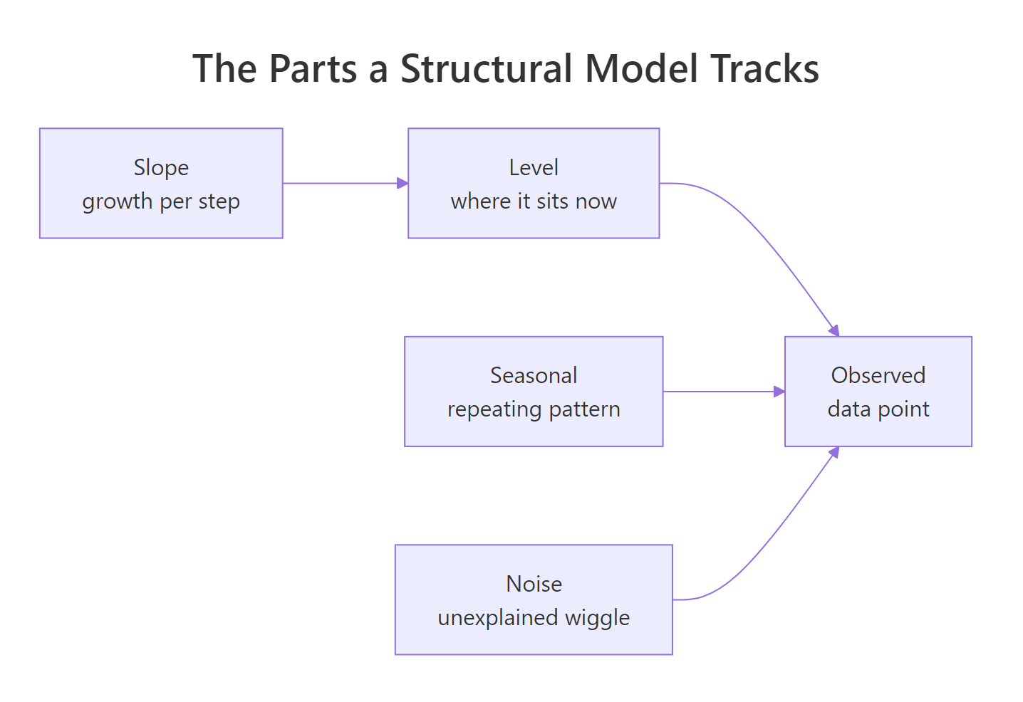
Figure 1: the slope adds to the level at each step, and the level, the seasonal term and the noise add up to the value you observe.
Now see the same three parts drawn over time, which is worth more than any table.
The level panel is a smooth upward curve with none of the summer sawtooth left in it. The seasonal panel holds a repeating shape that barely changes shape from year to year. The slope panel is a flat line, which is a genuine finding rather than a plotting artifact, and the next block explains why.
A structural model is controlled entirely by how much each part is allowed to move from one step to the next. That amount is a variance, and StructTS() estimates one per part.
Read those four numbers as speed limits. The level is allowed to drift a little each month (0.000772), the seasonal shape is allowed to drift about twice as much (0.001397), and the slope is allowed to move not at all (0.000000). A zero variance means that part is frozen: the growth rate is estimated once and then held fixed forever, which is why the slope panel was a flat line at 0.010.
Try it: The seasonal column swings between two extremes across the whole series. Report the smallest and largest value the fitted slope takes instead, and see whether it moves at all.
Click to reveal solution
Explanation: the smallest and largest values are the same number, so the slope never moves. That follows directly from its estimated variance of zero. The model concluded that a constant monthly growth rate of 0.0101 in log units, roughly 1% per month, plus a wandering level, explains this series better than a growth rate that changes.
How do you build a series from parts, and get them back again?
Reading components out of real data leaves one question open: where do they come from in the first place? The fastest way to answer that is to be the generator yourself. If you write the loop that produces the level, the slope and the season, then nothing about the model can stay mysterious, because you already know the true answer before any fitting happens.
Two rules define the whole family. The first says how an observation relates to the hidden parts:
$$y_t = \mu_t + \tau_t + \varepsilon_t$$
The second says how the hidden parts evolve from one step to the next:
$$\mu_t = \mu_{t-1} + \delta_{t-1} + \eta_t, \qquad \delta_t = \delta_{t-1} + \zeta_t$$
Where:
- $y_t$ = the value you actually observe at time $t$
- $\mu_t$ = the level, where the series sits once the season is stripped out
- $\delta_t$ = the slope, how much the level is expected to gain next step
- $\tau_t$ = the seasonal term for this position in the cycle
- $\varepsilon_t$, $\eta_t$, $\zeta_t$ = independent random shocks, one per part, each with its own variance
If the formulas are not your preferred language, skip them. The loop below is the same two rules written as R, and the code is the better explanation. Each step nudges the slope by a small random amount, then moves the level by the current slope plus its own small random amount.
The level started at 100 and finished at 120.03 after 96 quarters. The slope started at 0.5 per quarter and drifted down to 0.17, without anyone telling it to. That drift is the entire point of a local linear trend: growth is not assumed constant, it is allowed to decay or accelerate on its own.
Now add the two remaining ingredients. The seasonal pattern is a fixed four-quarter shape, and the noise is what stops the observed series from being a clean curve.
Quarter 1 is the high quarter in both years, and quarter 2 and quarter 4 are the low ones, matching the c(6, -2, -1, -3) shape we wrote. The values are not exactly level + season because rnorm(n, 0, 1) added a random amount to each one, which is the epsilon term.
Plotting the observed series next to the parts it was built from makes the relationship visible in one glance.
The top panel looks jagged and hard to read. The middle panel is the same series with the season and the noise removed, and it is a smooth climb. The bottom panel is the sawtooth that was hiding inside the top panel all along. A structural model's job is to reverse this picture: given only the top panel, reconstruct the other two.
Try it: How large is the seasonal effect in this series? Report the peak, the trough, and the gap between them, which is what a forecaster would call the seasonal swing.
Click to reveal solution
Explanation: the swing is 9 units, from a trough of -3 to a peak of 6. The final number confirms the design choice from the callout above: one full year of seasonal offsets sums to exactly 0, so the seasonal term adds nothing to the long-run level.
How does R recover parts it never observed?
You now have a series y and you know the truth behind it. Hand y to StructTS() and it sees only the top panel. How does it get the other two back?
The machinery is called the Kalman filter, and it works one time step at a time. It holds a current best guess of the level and slope, uses that guess to predict the next observation, compares the prediction with what actually arrived, and then nudges the guess in the direction of the error. A large surprise moves the guess a lot; a small surprise moves it a little. How much a given surprise moves the guess is decided by the variances, which is why those four numbers matter so much.
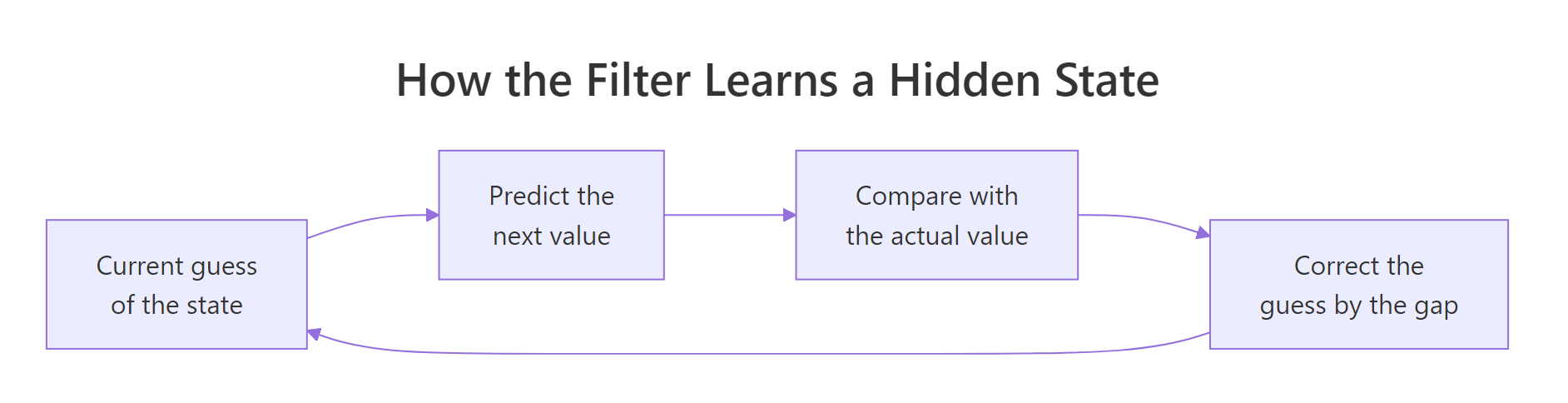
Figure 2: the filter guesses, predicts, compares with the actual value, and corrects the guess by part of the gap, once per time step.
Running that loop forward gives the filtered estimate, which uses only the past. Running a second pass backward over the whole series gives the smoothed estimate, which uses past and future together, and that is what tsSmooth() returns. Smoothed estimates are the right choice for understanding history; filtered estimates are the right choice for imitating what you would have known in real time. There is a full walkthrough of the recursion in the Kalman filter tutorial.
Fit the model to the simulated series and compare its four estimated variances against the values we actually used.
We generated the data with an observation noise of rnorm(n, 0, 1), which is a variance of 1. The model estimated 1.0382, so the noise level was recovered almost exactly. The other three are less flattering. We used a level variance of 0.04 and a slope variance of 0.0009, and the model reports 0.0000 for the level and 0.0620 for the slope, effectively swapping the two roles.
That looks alarming until you ask what actually matters. A wandering level and a wandering slope produce very similar looking paths, so the data cannot cleanly separate them. What the data can pin down is the combined path. Check that instead.
The recovered level tracks the true hidden level with a correlation of 0.9964 and a typical error of 0.48 units, on a series whose noise alone has a standard deviation of 1. The model reconstructed a quantity it never saw, to better accuracy than the noise on a single observation, by pooling information across all 96 quarters.
Try it: The level came back with a correlation of 0.996. Check the other hidden part: how closely does the recovered seasonal column match the true four-quarter pattern we wrote?
Click to reveal solution
Explanation: the seasonal term comes back at 0.997, marginally better than the level. Seasonality is the easiest component to recover because it repeats: every fourth quarter carries evidence about the same offset, so the filter gets 24 looks at each of the four numbers.
Where does the classical fit break, and why go Bayesian?
So far StructTS() has behaved well. Now give it a harder job, which is the job you actually care about: fit on part of the history and forecast the rest. We train on 1949 through 1958 and hold out the final two years of AirPassengers as a test set.
The variances came out completely differently from the full-sample fit. Earlier the level moved and the slope was frozen; now the level is frozen at 0.000000 and the slope is the part doing all the wandering, with a variance of 0.002405. Two of the four estimates sit exactly on zero, which is the edge of the allowed range rather than a value the data pointed to.
Watch what that does to a forecast.
The forecast declines month after month. It predicts 322 passengers for January 1959 and 61 for December 1960, on a series that had been climbing for a decade and in fact reached 432 that month. Because the slope was free to wander and happened to end the training window pointing down, the model extrapolated that downward slope for two solid years.
A mean absolute error of 300.5 passengers per month, against actual values in the 360 to 622 range, means the forecast is worse than useless.
Try it: Before judging a forecast, you need something to judge it against. A seasonal naive forecast just repeats the most recent full year. Compute its error on the same test set, using the final 12 months of the training window repeated twice.
Click to reveal solution
Explanation: repeating last year twice gives a mean absolute error of 71.25, four times better than the fitted structural model's 300.5. Any model that cannot beat this line does not deserve to be deployed. Keep the 71.25 in mind; it is the bar for the rest of this tutorial.
The problem is not the structural idea. The problem is committing to one guess about the variances. What we want is a method that carries every plausible set of variances forward at once, weights them by how well each explains the data, and averages the forecasts they produce. That is what a Bayesian treatment does, and it is what bsts is for.
How do you fit a bsts model and read its draws?
bsts stands for Bayesian structural time series. It was written by Steven L. Scott at Google, and it is the engine underneath the CausalImpact package. Instead of returning one estimate per variance, it returns thousands of draws from the range of variances the data finds credible.
bsts package needs compiled C++ code that the in-browser R build does not include, so these blocks are marked as static. Run install.packages("bsts") in RStudio and paste them in there. The outputs shown are from a real run, and the seeds are fixed, so you should reproduce them exactly.A model is built in two stages. First you describe the structure by growing a list of components. Then you hand that list to bsts().

Figure 3: every bsts analysis follows the same five steps, whatever components you choose.
library(bsts)
ss <- AddLocalLinearTrend(list(), train)
ss <- AddSeasonal(ss, train, nseasons = 12)
sapply(ss, function(component) class(component)[1])
#> [1] "LocalLinearTrend" "Seasonal"
Every Add* function takes an existing specification as its first argument and returns a longer one, which is why the pattern is ss <- AddSomething(ss, ...). Starting from list() means starting from no structure at all. The series is passed in as well because the functions use its scale to set sensible default priors. A prior is the model's starting belief about a quantity before it looks at the data, and here it amounts to a rough statement of how large each variance could plausibly be. nseasons = 12 says one full seasonal cycle is twelve observations.
Now fit it. This is where the sampling happens.
model <- bsts(train, state.specification = ss, niter = 1000, ping = 0, seed = 8675309)
dim(model$state.contributions)
#> [1] 1000    2  120
niter = 1000 asks for a thousand draws, ping = 0 silences the progress counter, and seed = 8675309 fixes the random stream so that rerunning the block gives identical results. Always set a seed, because a Bayesian fit that changes every time you run it is impossible to debug.
Those three numbers describe everything the fit produced: 1000 draws, 2 components, 120 time points. A draw is one complete, self-consistent answer to the question "what were the variances, and given those variances, what was the level and the season at every month?" bsts produces a thousand such answers, each slightly different, and their spread is the model's honest uncertainty.
The sampler alternates between two moves. Given a set of variances, it simulates a whole path for the hidden components; given those component paths, it draws a fresh set of variances. Repeating that a thousand times explores the whole range of explanations rather than settling on one, which is precisely the fix for the boundary collapse we just watched.
dimnames(model$state.contributions)[[2]]
#> [1] "trend"         "seasonal.12.1"
The two components you asked for come back labelled trend and seasonal.12.1. AddLocalLinearTrend() reports the level and the slope together under the single name trend, and seasonal.12.1 is the twelve-period season. These labels are how you pull one component out of the fit later, which the exercises at the end of this tutorial do.
bsts() and predict() each draw random numbers, and each takes its own seed argument. Fixing only the first still leaves your forecast wobbling between runs.Try it: Some series have short-term momentum that a level and a season cannot capture, and AddAr() adds an autoregressive component for exactly that. Add an AR(1) term to ss and confirm the specification now holds three components.
# Goal: build ss_ar with an AR(1) term added, then list its component classes.
# Hint: AddAr(ss, train, lags = 1) follows the same pattern as the other Add functions.
length(ss)
#> [1] 2
Click to reveal solution
ss_ar <- AddAr(ss, train, lags = 1)
sapply(ss_ar, function(component) class(component)[1])
#> [1] "LocalLinearTrend" "Seasonal"         "ArProcess"
Explanation: the specification is an ordinary list, so adding a component appends to it. The order you add components in does not matter to the fit; the sampler treats them as one combined state.
How do you read the posterior draws?
Not all thousand draws are usable. The sampler starts from an arbitrary position and needs time to find the region the data actually supports, and draws from that early stage would distort your estimates. Discarding them is called burn-in, and what remains is the posterior: the set of parameter values the model finds credible now that it has seen the data.
burn <- SuggestBurn(0.1, model)
burn
#> [1] 287
Note what happened there. SuggestBurn(0.1, model) is often described as "discard 10%", but it returned 287 out of 1000, not 100. The function looks at how the log likelihood climbed across the chain and reports where it stopped improving, so the answer is driven by this chain rather than by a fixed rule. On this series the sampler needed almost 300 iterations to settle, which is exactly the kind of thing a fixed 10% rule would have hidden.
With the warm-up gone, ask how well the model fits.
round(unlist(summary(model)[c("residual.sd", "prediction.sd", "rsquare", "relative.gof")]), 4)
#>   residual.sd prediction.sd       rsquare  relative.gof
#>        0.0184        0.0586        0.9978        0.6882
residual.sd of 0.0184 is the typical gap between the model's fitted value and the data, in log units, so roughly 1.9% in passenger terms. prediction.sd of 0.0586 is the larger and more honest number: it measures one-step-ahead errors, where the model has not yet seen the point it is guessing. rsquare of 0.9978 is flattering for the same reason most in-sample fit statistics are, and relative.gof of 0.6882 compares the model against a naive random walk, where 1 is perfect and 0 is no better than the walk.
Now for the thing StructTS could not give you. Every one of those component variances has a whole distribution behind it, so instead of one number you can ask for its range. One bookkeeping detail first: bsts stores these in the sigma.* slots as standard deviations, while StructTS reported variances. Square a bsts number before comparing it with a StructTS one.
draws <- cbind(obs   = model$sigma.obs[-(1:burn)],
               level = model$sigma.trend.level[-(1:burn)],
               slope = model$sigma.trend.slope[-(1:burn)],
               seas  = model$sigma.seasonal.12[-(1:burn)])
round(apply(draws, 2, quantile, probs = c(0.1, 0.5, 0.9)), 4)
#>        obs  level  slope   seas
#> 10% 0.0143 0.0221 0.0007 0.0016
#> 50% 0.0183 0.0262 0.0015 0.0042
#> 90% 0.0225 0.0303 0.0035 0.0084
Every column is a range rather than a point. The slope standard deviation sits between 0.0007 and 0.0035 with a middle value of 0.0015, so the model is confident the slope moves a little and confident it does not move much. Compare that with StructTS, which on this same training window put the level variance at exactly zero. Here the level standard deviation never comes near zero: even the 10% draw is 0.0221, a variance of about 0.0005, so not one draw supports a frozen level.
Try it: The table above reports the median observation noise as 0.0183 to four decimals. Get the median of the level standard deviation to five decimals instead.
# Goal: report the median of the level standard deviation to 5 decimals.
# Hint: this line does it for the observation noise; the level draws are in sigma.trend.level.
round(median(model$sigma.obs[-(1:burn)]), 5)
#> [1] 0.01832
Click to reveal solution
round(median(model$sigma.trend.level[-(1:burn)]), 5)
#> [1] 0.02617
Explanation: the level moves about 0.026 log units per month while the observation noise is about 0.018, so on this series the underlying level is genuinely more volatile than the measurement error around it.
How do you turn those draws into a forecast?
A forecast from bsts is not a formula evaluation. Each of the 713 surviving draws is a complete model, so predict() takes each one, runs it forward 24 months with fresh random shocks, and collects the resulting paths. The reported mean is the average over those paths, and the interval is a pair of quantiles across them.
pred <- predict(model, horizon = 24, burn = burn, quantiles = c(0.025, 0.975), seed = 1)
round(exp(pred$mean[1:6]), 1)
#> [1] 350.7 340.6 393.4 378.1 377.9 432.1
January 1959 is forecast at 350.7 passengers against an actual of 360, and June at 432.1 against an actual of 472. The forecast keeps climbing and keeps its seasonal shape, which is what the collapsed StructTS fit failed to do on identical data.
round(c(bsts_mae = mean(abs(exp(pred$mean) - exp(test)))), 2)
#> bsts_mae
#>    52.94
52.94 against 300.5 for StructTS on the same training window, and against 71.25 for the seasonal naive benchmark. Same components, same data, same 24-month horizon; the only change is averaging over the uncertainty in the variances instead of guessing at them once.
Point forecasts are the least interesting output. The interval is where a structural model earns its place.
round(exp(pred$interval[, c(1, 12, 24)]), 1)
#>        [,1]  [,2]  [,3]
#> 2.5%  322.9 263.0 192.2
#> 97.5% 381.5 464.8 633.1
One month out the model is confident: somewhere between 323 and 382, a span of about 59 passengers. Twelve months out the span has grown to about 202, and twenty-four months out to about 441. The interval widens because each extra step forward adds another round of unknown shocks, and because the parameter uncertainty compounds along with them. A forecast that quotes the same interval at every horizon is hiding one of those two effects.
Try it: The block above printed three horizons at once. Pull out just the 24-month-ahead interval and compute how wide it is in passengers.
# Goal: get the horizon-24 interval on its own, then subtract low from high.
# Hint: this line does it for horizon 1; interval has one column per horizon.
round(exp(pred$interval[, 1]), 1)
#>  2.5% 97.5%
#> 322.9 381.5
Click to reveal solution
round(exp(pred$interval[, 24]), 1)
#>  2.5% 97.5%
#> 192.2 633.1
round(unname(exp(pred$interval[2, 24]) - exp(pred$interval[1, 24])), 1)
#> [1] 440.9
Explanation: two years out the model will only commit to a range of 192 to 633 passengers, a width of 440.9. That is honest rather than weak, and the next section shows that a different trend component narrows it substantially.
Which trend component should you choose?
The interval above is wide because AddLocalLinearTrend() lets the slope random-walk with no anchor. Over 24 steps that slope can drift a long way, and the model correctly reports that it might. Three trend components handle this differently.
AddLocalLevel() has no slope at all. The level wanders, but there is no growth term to extrapolate, so long forecasts flatten out. AddLocalLinearTrend() adds a slope that random-walks freely, which tracks short-term changes in growth well and fans out over long horizons. AddSemilocalLinearTrend() gives the slope a long-run average and pulls it back toward that average, so short-term growth changes are still tracked but the slope cannot wander off forever.
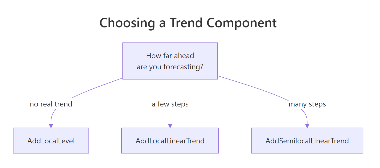
Figure 4: pick the trend component from how far ahead you need to forecast.
Rather than take that on faith, fit all three on the same training window and score them on the same held-out two years.
ss_ll <- AddSeasonal(AddLocalLevel(list(), train), train, nseasons = 12)
m_ll  <- bsts(train, state.specification = ss_ll, niter = 1000, ping = 0, seed = 8675309)
ss_sl <- AddSeasonal(AddSemilocalLinearTrend(list(), train), train, nseasons = 12)
m_sl  <- bsts(train, state.specification = ss_sl, niter = 1000, ping = 0, seed = 8675309)
c(local_level = SuggestBurn(0.1, m_ll), semilocal = SuggestBurn(0.1, m_sl))
#> local_level   semilocal
#>          37          15
Both alternatives settled far faster than the local linear trend did, needing 37 and 15 warm-up draws against 287. A sampler that converges quickly is usually a sign that the model is a comfortable fit for the data.
score <- function(fit) {
  b <- SuggestBurn(0.1, fit)
  p <- predict(fit, horizon = 24, burn = b, quantiles = c(0.025, 0.975), seed = 1)
  c(mae   = round(mean(abs(exp(p$mean) - exp(test))), 2),
    width = round(unname(exp(p$interval[2, 24]) - exp(p$interval[1, 24])), 1))
}
res <- rbind(local_level  = score(m_ll),
             local_linear = score(model),
             semilocal    = score(m_sl))
res
#>                mae width
#> local_level  73.63 201.8
#> local_linear 52.94 440.9
#> semilocal    27.50 268.0
The semilocal trend wins clearly: an error of 27.50 passengers per month, a little over half the local linear trend's 52.94 and less than a tenth of the collapsed StructTS fit's 300.5. It reaches that while quoting an interval of 268 rather than 441, so it is both more accurate and more decisive.
The local level model is the cautionary row. It has the narrowest interval at 201.8, and the worst error of the three at 73.63, which is actually worse than the 71.25 you get from simply repeating last year. Its interval is narrow because a model with no slope has nothing to be uncertain about, not because it knows more.
Try it: The table has two columns pointing in different directions. Identify which trend gives the narrowest interval, and whether the same trend also gives the lowest error.
# Goal: name the row with the smallest width, and the row with the smallest mae.
# Hint: this line reads one column; which.min gives you the winning row number.
res[, "mae"]
#>  local_level local_linear    semilocal
#>        73.63        52.94        27.50
Click to reveal solution
rownames(res)[which.min(res[, "width"])]
#> [1] "local_level"
rownames(res)[which.min(res[, "mae"])]
#> [1] "semilocal"
Explanation: they are different models. The narrowest interval belongs to the least accurate model, which is the clearest possible demonstration that confidence and correctness are separate properties.
How do you add predictors with a spike-and-slab prior?
Everything so far used the series' own past. bsts also accepts predictors through an ordinary formula interface, which is what makes it a nowcasting tool: if a related indicator is available before your target series is published, the model can lean on it.
The package ships a real example. initial.claims holds weekly US unemployment insurance claims alongside ten Google search popularity series that were found to correlate with it.
data(iclaims)
dim(initial.claims)
#> [1] 456  11
colnames(initial.claims)[1:5]
#> [1] "iclaimsNSA"                "michigan.unemployment"     "idaho.unemployment"
#> [4] "pennsylvania.unemployment" "unemployment.filing"
456 weeks, one response column and ten candidate predictors. Look at the values before modelling them.
round(head(initial.claims[, 1:3], 3), 3)
#>            iclaimsNSA michigan.unemployment idaho.unemployment
#> 2004-01-04      2.536                 1.488             -0.561
#> 2004-01-11      0.882                 1.100             -0.992
#> 2004-01-18 -0.077 1.155 -1.212Ten predictors for one response is the setting where ordinary regression starts inventing relationships. bsts handles it with a spike-and-slab prior. The spike is a lump of probability sitting exactly on zero, saying "this predictor is probably irrelevant"; the slab is a wide distribution for the coefficient in the event that it is relevant. On each draw, the sampler decides for each predictor which side it falls on, so the model is choosing its variables a thousand times rather than once.
expected.model.size sets how many predictors you expect to survive that choice, and it controls how heavy the spike is.
ss_r <- AddLocalLinearTrend(list(), initial.claims$iclaimsNSA)
ss_r <- AddSeasonal(ss_r, initial.claims$iclaimsNSA, nseasons = 52)
mr <- bsts(iclaimsNSA ~ ., state.specification = ss_r, data = initial.claims,
           niter = 1000, expected.model.size = 3, ping = 0, seed = 4321)
burn_r <- SuggestBurn(0.1, mr)
burn_r
#> [1] 433
The formula iclaimsNSA ~ . means "use every other column as a predictor". This fit takes about 45 seconds because a 52-week seasonal component carries 51 hidden states and the sampler must draw all of them a thousand times.
Because variable selection happened on every draw, the natural summary is the fraction of draws in which each predictor was included.
inclusion <- colMeans(mr$coefficients[-(1:burn_r), ] != 0)
round(sort(inclusion, decreasing = TRUE)[1:5], 3)
#>        idaho.unemployment       unemployment.office pennsylvania.unemployment
#>                     1.000                     1.000                     0.035
#>       unemployment.filing     illinois.unemployment
#>                     0.025                     0.023
Two predictors were selected in every single draw, and the third-placed candidate appears in 3.5% of them. That is a decisive verdict, and it is more informative than a table of p-values: across the 567 draws kept after burn-in, there was not one in which idaho.unemployment or unemployment.office was left out.
For the two survivors, ask how large the effect is when it is present.
kept <- mr$coefficients[-(1:burn_r), ]
avg  <- apply(kept, 2, function(col) if (any(col != 0)) mean(col[col != 0]) else 0)
round(avg[names(sort(inclusion, decreasing = TRUE))[1:2]], 4)
#>  idaho.unemployment unemployment.office
#>              0.1211              0.5541
A one standard deviation rise in searches for unemployment.office goes with a 0.55 standard deviation rise in claims, and idaho.unemployment contributes a smaller 0.12. Averaging only over the draws where the coefficient is non-zero matters: averaging over all draws would drag a genuinely useful predictor toward zero purely because it was occasionally excluded.
Try it: expected.model.size = 3 translates into a prior probability that each individual predictor is included. Work out what that probability is for this fit.
# Goal: compute expected.model.size divided by the number of coefficients.
# Hint: this line gives you the denominator you need.
ncol(mr$coefficients)
#> [1] 11
Click to reveal solution
round(3 / ncol(mr$coefficients), 3)
#> [1] 0.273
Explanation: each predictor starts with a 27.3% chance of being in the model, since 3 expected predictors spread over 11 coefficients gives 3/11. The data then pushed two of them to 1.000 and the rest below 0.04, which is a large update away from the prior and therefore strong evidence.
How do you check whether the model is any good?
Comparing models on a single 24-month holdout is thin evidence. One unusual year can crown the wrong winner. The stronger test uses one-step-ahead prediction errors, which score the model at every point in the series rather than at one arbitrary split.
errors_llt <- bsts.prediction.errors(model, burn = burn)$in.sample
errors_ll  <- bsts.prediction.errors(m_ll, burn = SuggestBurn(0.1, m_ll))$in.sample
round(c(local_linear = mean(abs(colMeans(errors_llt))),
        local_level  = mean(abs(colMeans(errors_ll)))), 5)
#> local_linear  local_level
#>      0.04106      0.04032
This result deserves a pause. The local level model, which was the worst of the three at forecasting two years ahead, is very slightly better at predicting one month ahead. That is not a contradiction. Predicting one step needs a model that tracks the recent past closely, and predicting two years needs a model whose trend behaves sensibly when extrapolated. A component can be good at one and poor at the other.
CompareBstsModels() plots how each model's error accumulates across the series, and returns the underlying matrix.
pdf(NULL)
cmp <- CompareBstsModels(list("local level" = m_ll, "local linear" = model), burn = burn)
invisible(dev.off())
dim(cmp)
#> [1]   2 120
Two models, 120 time points, each entry the running total of absolute one-step error up to that point. Reading the same column for both models tells you who was ahead at that date, and reading across the row tells you when each model gained or lost ground.
Try it: Compare the two models halfway through the series and at the end. Print the cumulative error at time 120 and see whether the ranking at the midpoint still holds.
# Goal: read column 120 of cmp instead of column 60.
# Hint: cmp is an ordinary matrix, so cmp[, 60] is the midpoint.
round(cmp[, 60], 3)
#> [1] 2.974 3.001
Click to reveal solution
round(cmp[, 120], 3)
#> [1] 4.843 4.927
Explanation: the local level model leads at the midpoint (2.974 against 3.001) and still leads at the end (4.843 against 4.927), so its small one-step advantage is consistent rather than lucky. It remains the worse choice for a two-year forecast, which is the whole lesson of this section.
Complete Example: forecast air passengers end to end
Here is the full workflow in one block, using the component that won: a semilocal linear trend for the long horizon, plus a twelve-month season. Build the specification, fit, discard the warm-up, forecast, and score.
final_ss   <- AddSeasonal(AddSemilocalLinearTrend(list(), train), train, nseasons = 12)
final_fit  <- bsts(train, state.specification = final_ss, niter = 1000, ping = 0, seed = 20260723)
final_burn <- SuggestBurn(0.1, final_fit)
final_pred <- predict(final_fit, horizon = 24, burn = final_burn,
                      quantiles = c(0.025, 0.975), seed = 7)
round(c(burn   = final_burn,
        mae    = mean(abs(exp(final_pred$mean) - exp(test))),
        low24  = exp(final_pred$interval[1, 24]),
        high24 = exp(final_pred$interval[2, 24])), 2)
#>         burn          mae   low24.2.5% high24.97.5%
#>        15.00        27.50       309.17       577.13
Fifteen warm-up draws discarded, a mean absolute error of 27.50 passengers per month over two unseen years, and a two-year-ahead interval running from 309 to 577. December 1960 actually came in at 432, comfortably inside that range.
Practice Exercises
Exercise 1: Does the log transform earn its keep?
Every model in this tutorial was fitted to log(AirPassengers). Fit the same semilocal trend plus seasonal model to the raw, untransformed series over the same 1949 to 1958 window, forecast 24 months, and compute the mean absolute error against the raw test values. Compare it with the 27.50 the log-scale model achieved.
# Build raw_train and raw_test from AirPassengers with window().
# Hint: no exp() is needed anywhere, because you never took a log.

# Write your code below:
Click to reveal solution
raw_train <- window(AirPassengers, end = c(1958, 12))
raw_test  <- window(AirPassengers, start = c(1959, 1))
my_ss   <- AddSeasonal(AddSemilocalLinearTrend(list(), raw_train), raw_train, nseasons = 12)
my_fit  <- bsts(raw_train, state.specification = my_ss, niter = 1000, ping = 0, seed = 11)
my_burn <- SuggestBurn(0.1, my_fit)
my_pred <- predict(my_fit, horizon = 24, burn = my_burn, seed = 3)
round(c(raw_scale_mae = mean(abs(my_pred$mean - raw_test))), 2)
#> raw_scale_mae
#>          86.6
Explanation: 86.6 against 27.50, so the log transform is worth more than three times the model's entire accuracy. The reason is that an additive seasonal component assumes the summer bump is the same size every year. On the raw scale it is not: the bump grows with the series. Taking logs converts that multiplying pattern into an adding one, which is the assumption the model was built on.
Exercise 2: Recover a seasonal pattern you already know
Fit a local level plus seasonal model with bsts to the simulated quarterly series y from the second section, using nseasons = 4. Pull the seasonal component out of state.contributions, average it across draws, and compute the swing across the first four quarters. Compare it against the true swing of 9 that you built into the data.
# The component you want is named "seasonal.4.1" in state.contributions.
# Hint: colMeans over the draws dimension gives a posterior mean per time point.

# Write your code below:
Click to reveal solution
my_sim_ss   <- AddSeasonal(AddLocalLevel(list(), y), y, nseasons = 4)
my_sim_fit  <- bsts(y, state.specification = my_sim_ss, niter = 1000, ping = 0, seed = 5)
my_sim_burn <- SuggestBurn(0.1, my_sim_fit)
my_season   <- colMeans(my_sim_fit$state.contributions[-(1:my_sim_burn), "seasonal.4.1", ])
round(c(recovered_swing = max(my_season[1:4]) - min(my_season[1:4]),
        true_swing      = max(season) - min(season)), 2)
#> recovered_swing      true_swing
#>            8.46            9.00
Explanation: the model recovered a swing of 8.46 against a true 8 to 9 unit swing, with the shortfall coming from the first few quarters where the filter is still finding its footing. The seasonal estimate tightens up considerably further into the series, which is why the very start of a fitted component is the part to trust least.
Exercise 3: How often do the two survivors appear together?
The claims model gave both idaho.unemployment and unemployment.office an inclusion probability of 1.000 individually. That does not automatically mean they were always selected in the same draw. Using mr$coefficients, compute the fraction of post-burn draws where both are non-zero at once, then tabulate how many predictors each draw selected in total.
# Hint: a coefficient matrix comparison like kept[, "x"] != 0 gives a logical vector,
# and rowSums over a logical matrix counts the selected predictors per draw.

# Write your code below:
Click to reveal solution
my_kept <- mr$coefficients[-(1:burn_r), ]
my_top2 <- names(sort(colMeans(my_kept != 0), decreasing = TRUE))[1:2]
round(mean(my_kept[, my_top2[1]] != 0 & my_kept[, my_top2[2]] != 0), 3)
#> [1] 1
table(rowSums(my_kept != 0))
#>   2   3   4
#> 501  64   2
Explanation: they do appear together in every draw, so the joint probability is 1. The table shows the sampler chose exactly two predictors in 501 of the 567 kept draws, three in 64, and four in only 2. The prior said to expect three; the data pulled that down to two and stayed there.
Frequently Asked Questions
Is bsts the same thing as CausalImpact? No, but they are closely related. CausalImpact uses bsts internally to build a forecast of what a series would have done without some intervention, then compares that counterfactual against what actually happened. Learning bsts first makes CausalImpact far easier to reason about, and there is a dedicated CausalImpact walkthrough once you are ready.
How many iterations do I need? Start at 1000, check what SuggestBurn() returns, and raise niter if the suggested burn-in is a large fraction of it. In this tutorial one model burned 287 of 1000 while another burned 15, on the same data, purely because of the trend component. If burn-in consumes more than half the chain, you are keeping too few draws to trust the quantiles.
Does bsts handle missing values? Yes, and this is one of the strongest practical arguments for state space models. A missing observation simply means the filter skips its correction step for that time point and carries the prediction forward, so no imputation is required. Pass NA values through and the model handles them.
Can it handle more than one seasonal period? Yes. Call AddSeasonal() more than once with different nseasons values, and use the season.duration argument when one cycle spans several observations, such as a day-of-week pattern in hourly data. AddTrig() provides a trigonometric alternative that uses far fewer states for long seasonal periods.
How is this different from decompose() or stl()? Those functions split a series into trend, seasonal and remainder using moving averages or a loess smoother. They describe the history you already have and stop there: they cannot forecast, they attach no uncertainty to the parts, and they cannot take predictors. A structural model instead states how the parts are generated and estimates the variances that drive them, so the same fitted object gives you the components and a forecast, each with an interval around it.
Should I use ARIMA or a structural model? Use ARIMA when you want a compact model of the correlation structure and you are forecasting a short way ahead. Use a structural model when you need the components themselves, when you want to add predictors with automatic variable selection, or when you have missing data. The two overlap heavily in accuracy, so let the requirement decide rather than the fashion. There is a full treatment in the ARIMA tutorial.
Why do the bsts blocks not run in the browser here? bsts depends on a large compiled C++ library, and the browser R build only carries packages that have been compiled for it. Base R, stats, and the whole first half of this tutorial run in the page; the bsts blocks are marked static and are meant to be pasted into RStudio.
Summary
| Function | Component or job | Reach for it when |
|---|---|---|
StructTS(x, type = "BSM") |
Classical level, slope and season fit | You want a fast look at the components with no extra packages |
AddLocalLevel() |
Wandering level, no slope | The series has no persistent direction |
AddLocalLinearTrend() |
Level plus a freely wandering slope | Forecasting a few steps ahead |
AddSemilocalLinearTrend() |
Slope pulled back to a long-run rate | Forecasting far ahead, which was the winner here |
AddSeasonal(nseasons = k) |
Repeating pattern of length k | The series has a cycle |
AddAr(lags = 1) |
Short-term momentum | Residuals still show correlation |
bsts(..., niter, seed) |
Draws samples from the model | Always, and always with a seed |
SuggestBurn(0.1, model) |
How many warm-up draws to drop | Before reading any output |
predict(model, horizon, burn, seed) |
Forecast with credible intervals | The reason you fitted the model |
expected.model.size |
Spike-and-slab sparsity | You have more predictors than you trust |
bsts.prediction.errors() |
One-step-ahead errors | Comparing models honestly |
The workflow never changes: describe the structure as a list of components, fit it, drop the warm-up draws, read the components, then forecast. What changes between problems is which components you list, and the scoreboard from this tutorial shows how much that choice is worth: 300.5 mean absolute error for the classical fit that collapsed, 71.25 for repeating last year, 52.94 for a local linear trend, 27.50 for a semilocal one.
References
- Scott, S. L.
bsts: Bayesian Structural Time Series. CRAN package page, the canonical source for the current version, dependencies and vignettes. Link bstsreference manual (full argument documentation for everyAdd*function). Link- Scott, S. L. Fitting Bayesian structural time series with the
bstsR package. Unofficial Google Data Science Blog (2017). Link - R Core Team.
StructTS: Fit Structural Time Series. R manual. Link - R Core Team.
KalmanLikeand friends: Kalman filtering in base R. R manual. Link - Brodersen, K. et al. CausalImpact: inferring causal effects with Bayesian structural time series. Link
- Hyndman, R. J. and Athanasopoulos, G. Forecasting: Principles and Practice, 3rd edition, chapter on exponential smoothing state space models. Link
- Bayesian structural time series: model definition and history. Link
Continue Learning
- Kalman Filter in R walks through the predict-and-correct recursion that powers every fit in this tutorial, one step at a time.
- CausalImpact in R puts
bststo work estimating the effect of an intervention by forecasting the world in which it never happened. - ETS Models in R covers exponential smoothing, the other major state space family, and shows where it overlaps with the structural models here.