Forecast Value Added: When Human Judgment Helps
Forecast Value Added (FVA) is a simple audit that asks one question of every step in your forecasting process: did this step make the forecast more accurate than the step before it? A step that beats the previous one has positive FVA and earns its place. A step that makes the forecast worse has negative FVA and is quietly costing you money.
Most forecasting processes are a chain of steps. A computer produces a statistical forecast, then a human reviews it and nudges the numbers up or down. Each step takes time and salary. FVA is how you find out which steps actually help and which ones just add noise. Everything in this tutorial runs in the code boxes right on this page, so you can change a number and re-run it. We use base R for the first four sections and the forecast package in the last one.
What is Forecast Value Added, and why should you measure it?
Think of your forecast as passing through a relay of hands. First a naive rule of thumb, then a statistical model, then an analyst who overrides the model. FVA checks each hand in turn and asks whether it improved accuracy or made it worse. The trick is that you always compare a step to a cheaper alternative, so a step only "wins" if it beats something you could have done for free.
That free alternative is the naive forecast. It is the placebo in a drug trial: if an expensive treatment cannot beat a sugar pill, the treatment is not working. In forecasting, the classic placebo is the random walk, where next month's forecast is simply this month's actual value. If your fancy model cannot beat "next month looks like this month," the model is not adding value.
Let's make this concrete. Below is one product's demand over 12 months, together with three competing forecasts of that same demand: the naive random walk, a statistical model, and the analyst's overridden numbers. Run it to see all four side by side.
Here is how to read the table. The actual column is what really sold each month. The naive column just copies last month's actual forward, which is why naive in month 2 is 102, the actual from month 1 (month 1 uses the prior December value of 100). The statistical column is a smooth model, and the override column is what the analyst submitted after editing the model.
One month stands out. Month 8 jumped to 165 because of a promotion, and you can already see the forecasts disagree wildly there. Hold that thought, because month 8 turns out to be the whole story.
The relay of hands is easier to picture as a ladder, where each rung is judged against the rung below it.

Figure 1: The FVA ladder: each step is judged against the step before it.
Try it: Compute the size of each month's miss for the statistical forecast, which is the absolute difference between the actual value and the statistical forecast.
Click to reveal solution
Explanation: abs() turns each difference into a positive size of the miss. Notice month 8 has an error of 45, far bigger than any other month, because the model never saw the promotion coming.
How do you measure whether a forecast is any good?
Before you can say one forecast beats another, you need a single number that scores accuracy. The most common one in demand planning is the Mean Absolute Percentage Error, or MAPE. It answers a plain question: on average, by what percentage did the forecast miss?
The recipe is short. For each month, take the miss, divide it by the actual value to turn it into a percentage, drop the sign, and average those percentages across all months. Writing it as a formula makes the steps explicit.
$$\text{MAPE} = \frac{100}{n} \sum_{t=1}^{n} \left| \frac{A_t - F_t}{A_t} \right|$$
Where:
- $A_t$ = the actual value in period $t$
- $F_t$ = the forecast for period $t$
- $n$ = the number of periods you are scoring
Lower MAPE is better, because it means the forecast missed by a smaller percentage. Let's write that recipe as a function and score all three forecasts at once.
Read the three numbers as report cards. The naive forecast missed by 10.5% on average, which is our floor to beat. The statistical model cut that almost in half to 5.9%, so the model is clearly doing something useful. The override, at 9.0%, is better than naive but noticeably worse than the model it started from.
That last comparison is the surprise. The analyst took a 5.9% forecast and handed back a 9.0% forecast. On the whole, the human editing made things worse. We will pin down exactly where that damage happened in a moment.
Try it: Some teams prefer Mean Absolute Error (MAE), the average miss in plain units instead of percentages. Complete the function so it returns the MAE, then score the override.
Click to reveal solution
Explanation: MAE drops the "divide by actual" step, so the answer stays in units. The override was off by about 10.5 units per month on average. MAE and MAPE often tell the same story, but MAE keeps the original scale.
How do you calculate Forecast Value Added?
Now we can define FVA precisely. Forecast Value Added is just the drop in error that a step produced compared to a benchmark. Because error is bad, a drop in error is good, so we subtract the step's error from the benchmark's error.
$$\text{FVA} = \text{error}_{\text{benchmark}} - \text{error}_{\text{step}}$$
A positive FVA means the step lowered the error and added value. A negative FVA means the step raised the error and destroyed value. In a real process you report two FVA numbers for each step: one against the naive floor, and one against the step immediately before it. Let's build that standard table, which practitioners call the FVA stairstep report.
Walk down the table one row at a time. The naive row is the baseline, so its FVA cells are blank. The statistical row shows fva_vs_naive of 4.6, meaning the model cut MAPE by 4.6 points versus naive. That is a strong, positive result: the model earns its keep.
The override row is where the process leaks. Its fva_vs_naive is 1.5, still positive, so at a glance the analyst looks helpful. But look at fva_vs_stat, which is -3.1. Compared to the model it actually edited, the override added 3.1 points of error. The analyst was measured against the wrong yardstick and looked fine, when in truth the editing set the forecast back.
Try it: Confirm the override's value against the naive baseline directly. Compute the naive MAPE minus the override MAPE and round to one decimal.
Click to reveal solution
Explanation: The override beat the naive floor by 1.5 points, which matches the fva_vs_naive cell in the table. The problem is not that the analyst lost to naive, it is that the analyst lost to the model.
When does human judgment actually help?
The overall numbers make the analyst look like a net drag. But averages hide as much as they reveal. To find out where the human helped and where they hurt, split the months into two groups: the single promotion month, when the analyst knew about a marketing push the model could not see, and the routine months, when the analyst was just tweaking a stable forecast.
Now the split makes it clear. On the promotion month the model missed badly, off by 27.3%, because it had no way to know a promotion was coming. The analyst, who did know, cut that miss to 3.0%, an enormous FVA of 24.3 points. This is human judgment at its best: the person had information the model simply did not have.
On routine months the picture flips. The model was already sharp at 3.9%, and the analyst's tinkering pushed the error up to 9.6%, an FVA of -5.7 points. With nothing special to add, the human was just injecting noise into an already-good forecast.
So the answer to the title is precise. Human judgment helps when the human knows something the model cannot know, such as a promotion, a new competitor, or a one-off event. It hurts when the human overrides a stable forecast out of habit. The quadrant below sums up the rule.
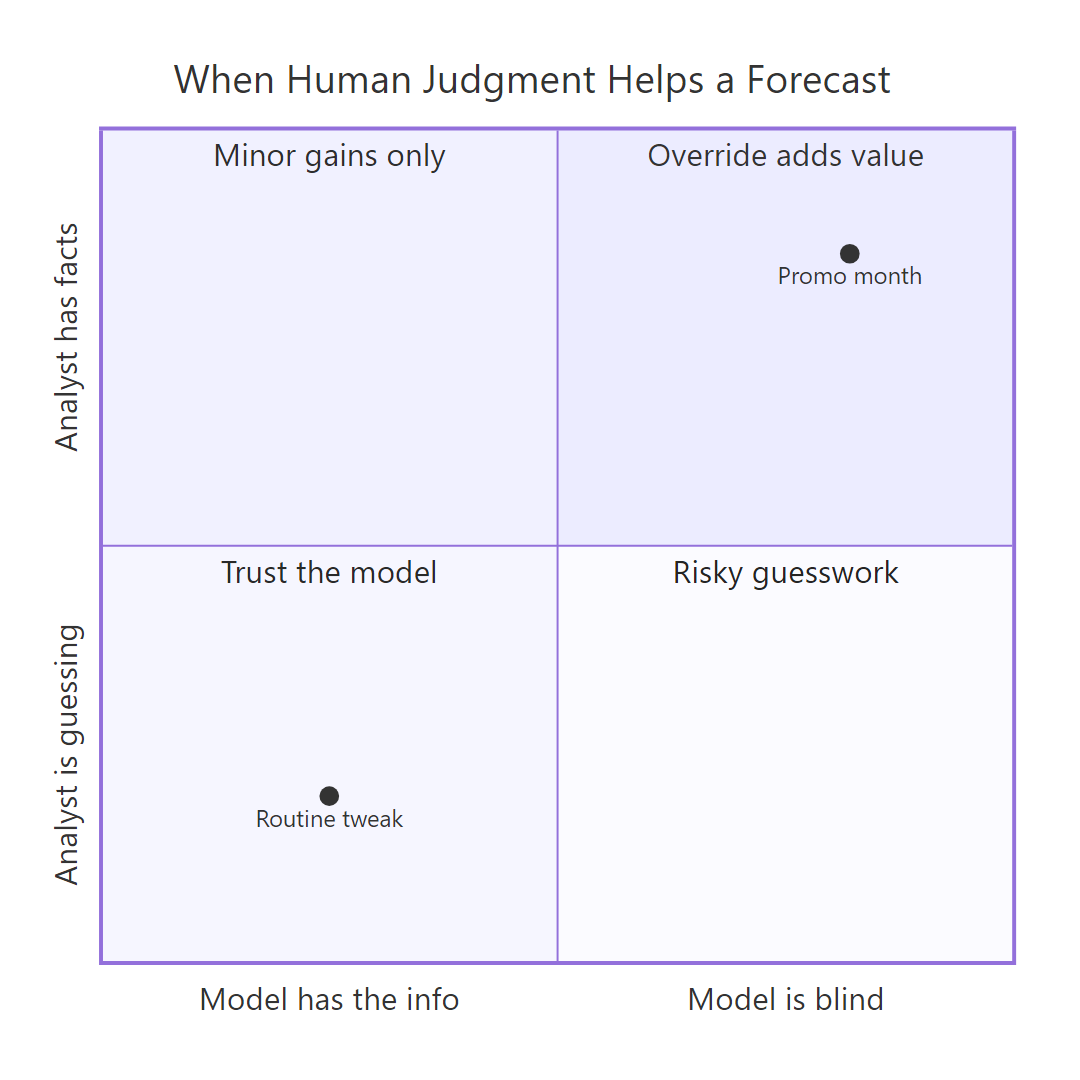
Figure 2: Human overrides add value only when the analyst knows something the model does not.
Try it: Count how many of the routine months the override missed by more than the model did. A high count confirms the tinkering was almost always harmful.
Click to reveal solution
Explanation: There are 11 routine months, and the override was worse on every single one. The analyst added value on exactly one month out of twelve, and it happened to be the month that mattered most.
How do you run an FVA analysis on real forecasts?
The example so far used hand-picked numbers so the lesson was clear. In practice you generate the naive and statistical forecasts yourself, then test any override on data the models never saw. Let's do that with the forecast package and the built-in AirPassengers series of monthly airline passengers.
The method is standard. Train the models on the early years, hold out the last two years as a test set, and score each forecast on that untouched holdout. We use a seasonal naive forecast as the baseline, an automatically chosen exponential smoothing model as the statistical step, and an analyst who expects continued route expansion and lifts the model by 5%.
The window() function slices the series by date, so train holds every month through the end of 1958 and test holds 1959 onward. The snaive() function repeats last year's same month as the forecast, a sensible floor for seasonal data, and ets() fits an exponential smoothing model automatically. Both snaive() and forecast() return an object that keeps its point predictions in a $mean component, which is the column we score and the one the analyst multiplies by 1.05. We reuse the same mape() function from earlier, so nothing new to learn there. Now turn those three MAPEs into the same stairstep report.
Here the human comes out ahead. The statistical model beat seasonal naive by 2.2 points, and the analyst's 5% lift beat the model by another 3.7 points. Why did the override help this time? The exponential smoothing model damped the upward trend, so it under-forecast a business that was still growing fast. The analyst knew growth was continuing and corrected exactly that blind spot. This is the same lesson as the promotion month, on real data: the override won because the human supplied information the model had discounted.
Try it: Not every hunch is right. Suppose a different analyst feared a slump and trimmed the model by 5% instead. Compute that override's FVA against the statistical model.
Click to reveal solution
Explanation: Trimming the forecast on a growing series made it worse, for an FVA of -4.3 points. Same tool, opposite result: the upward edit helped because it matched what actually happened, the downward edit hurt because it did not. FVA measures only the accuracy of the final number, not the reasoning behind the edit.
Practice Exercises
These combine the pieces above. The mape() function you wrote earlier is still available, so lean on it.
Exercise 1: Build the stairstep for a new product
A second product has its own promotion in month 8. Build the full FVA stairstep table for it: MAPE for each step, plus FVA versus naive and versus the statistical model.
Click to reveal solution
Explanation: Same pattern as the tutorial. The model added 6.5 points over naive, but the override gave back 2.2 of them, so this product has the same leaky-override problem.
Exercise 2: Write a reusable FVA reporter
Turn the stairstep logic into a function. Write fva_report() that takes the actuals, a named list of forecasts, and the name of the benchmark, and returns a data frame of MAPE and FVA versus that benchmark for every forecast.
Click to reveal solution
Explanation: sapply() runs the MAPE calculation over every forecast in the list at once. Indexing mapes[benchmark] grabs the benchmark's score, and subtracting each MAPE from it gives the FVA column. Now any process can be scored with one call.
Exercise 3: Find the override's best month
The override was harmful in most months but helpful in one. Find the single month where the override reduced the error the most compared to the statistical model, and report how many units of error it saved.
Click to reveal solution
Explanation: my_change is positive when the override missed by more than the model. The most negative value is the override's best moment, and which.min() finds it: month 8, the promotion, where the override cut the error by 40 units. One well-informed edit paid for the whole review process.
Frequently Asked Questions
What counts as a good FVA value?
Any FVA above zero means the step helped, so zero is the bar. In practice, a statistical model should show a clearly positive FVA against naive, and you want each human step to show a positive FVA against the step it edited. A step sitting near zero is a candidate for removal, because it costs effort without moving accuracy.
Which naive forecast should I use as the benchmark?
Use the simplest forecast that respects your data's pattern. For data without seasonality, the random walk (this period equals last period) is standard. For seasonal data like monthly sales, a seasonal naive forecast (this month equals the same month last year) is fairer, which is why the airline example used snaive().
Does a negative FVA mean we should fire the analysts?
No. It means you should redirect their effort. The segmented analysis showed the same analyst adding huge value on the promotion month and destroying value on routine months. The goal is to stop overriding stable forecasts and concentrate human attention on the events that models cannot see.
Is MAPE the only metric I can use for FVA?
Not at all. FVA works with any error metric, including MAE, RMSE, or weighted variants. Just keep the metric fixed across every row of a stairstep report so the comparisons are apples to apples. MAPE is popular because its percentages compare cleanly across products of different sizes.
How much history do I need before I trust an FVA result?
One month is an anecdote, not evidence. The 12-month examples here illustrate the mechanics, but for a real decision you want many periods and, ideally, many products, so a lucky override does not fool you. Segment the results by event type so consistent patterns, rather than one-off wins, drive your changes.
Summary
Forecast Value Added turns a vague worry ("is our forecasting process worth the effort?") into a number you can act on. The workflow is short and repeatable.
| Step | What you do | What it tells you |
|---|---|---|
| Pick a benchmark | Choose a naive forecast (random walk or seasonal naive) | The free floor every step must beat |
| Score each step | Compute MAPE for naive, statistical, and override | The accuracy report card |
| Build the stairstep | FVA = benchmark error minus step error | Which steps add value, which destroy it |
| Compare to the previous step | Score each step against the one before it, not just naive | Catches value-destroying overrides |
| Segment the results | Split by event type (promo vs routine) | Where human judgment truly helps |
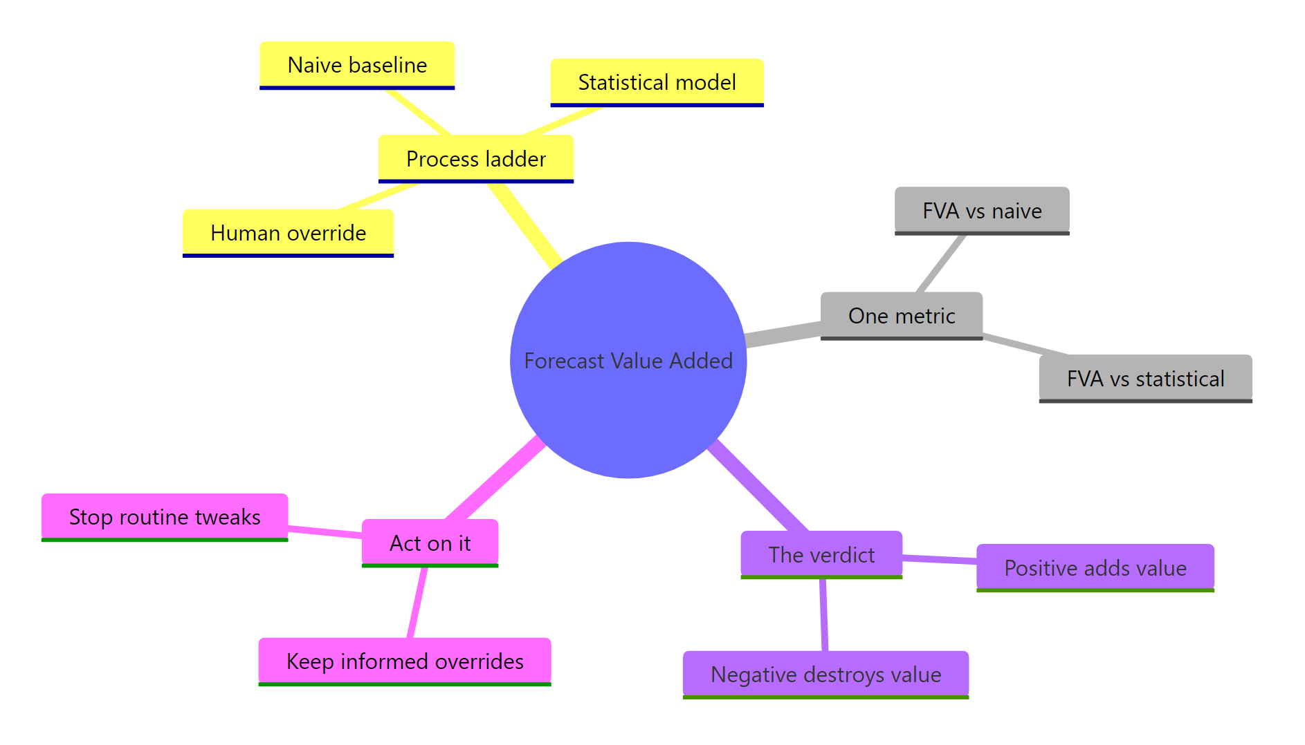
Figure 3: Forecast Value Added at a glance.
The headline lesson is about people, not math. Human overrides are worth it precisely when the human knows something the model cannot, such as a promotion or a structural change. When they are just editing a stable forecast, they tend to add noise. FVA is how you tell the two apart and put everyone's effort where it pays off.
References
- Gilliland, M. Forecast Value Added Analysis: Step by Step. SAS white paper. Link
- Hyndman, R.J. & Athanasopoulos, G. Forecasting: Principles and Practice, 3rd ed. Evaluating forecast accuracy. Link
- Hyndman, R.J. & Athanasopoulos, G. Forecasting: Principles and Practice, 3rd ed. Some simple forecasting methods (naive benchmarks). Link
- Hyndman, R.J. et al. forecast: Forecasting Functions for Time Series and Linear Models. CRAN. Link
- Hyndman, R.J. forecast package documentation. Link
- Hyndman, R.J. Show me the evidence (on evidence-based forecasting and simple benchmarks). Link
- Lokad. Forecast Value Added (FVA). Link
Continue Learning
- Forecast Accuracy in R: a deeper look at MAPE, MAE, RMSE, and how to choose the right error metric for your data.
- Benchmark Forecasts in R: how to build the naive and seasonal-naive baselines that every FVA analysis starts from.
- Monitoring Forecast Models in Production: once your process adds value, this shows how to watch it over time and catch accuracy drift.