Forecasting Through Structural Breaks in R
A structural break is a moment when the rule that generates your data changes: the average may jump to a new level or a steady trend may suddenly bend. A forecast trained on the old rule then drifts wrong. This tutorial shows you how to spot a break in R and forecast right through it.
What is a structural break, and why does it wreck a forecast?
Almost every forecasting method assumes the future behaves like the past. That assumption quietly breaks the moment something structural changes: a competitor exits, a pricing policy flips, a pandemic starts, a product goes viral. Analysts call that moment a structural break, and if you feed a model history from both sides of it, the model splits the difference between the two regimes and describes neither well. Let's build a series with a break so you can see the problem before we fix it.
We simulate ten years of monthly sales. For the first 72 months the average sits near 100 units. Then, at month 73, it jumps permanently to 150, the kind of shift a new distribution deal would cause. We load the two packages, then build the series and plot it.
The plot shows a flat band near 100 that suddenly steps up to a flat band near 150 at the red dashed line. The two numbers confirm it: the average was 99.2 before the break and 149.7 after. Nothing gradual happened, the level simply shifted. That single jump is the whole problem, and it comes in three flavours you will meet again and again.
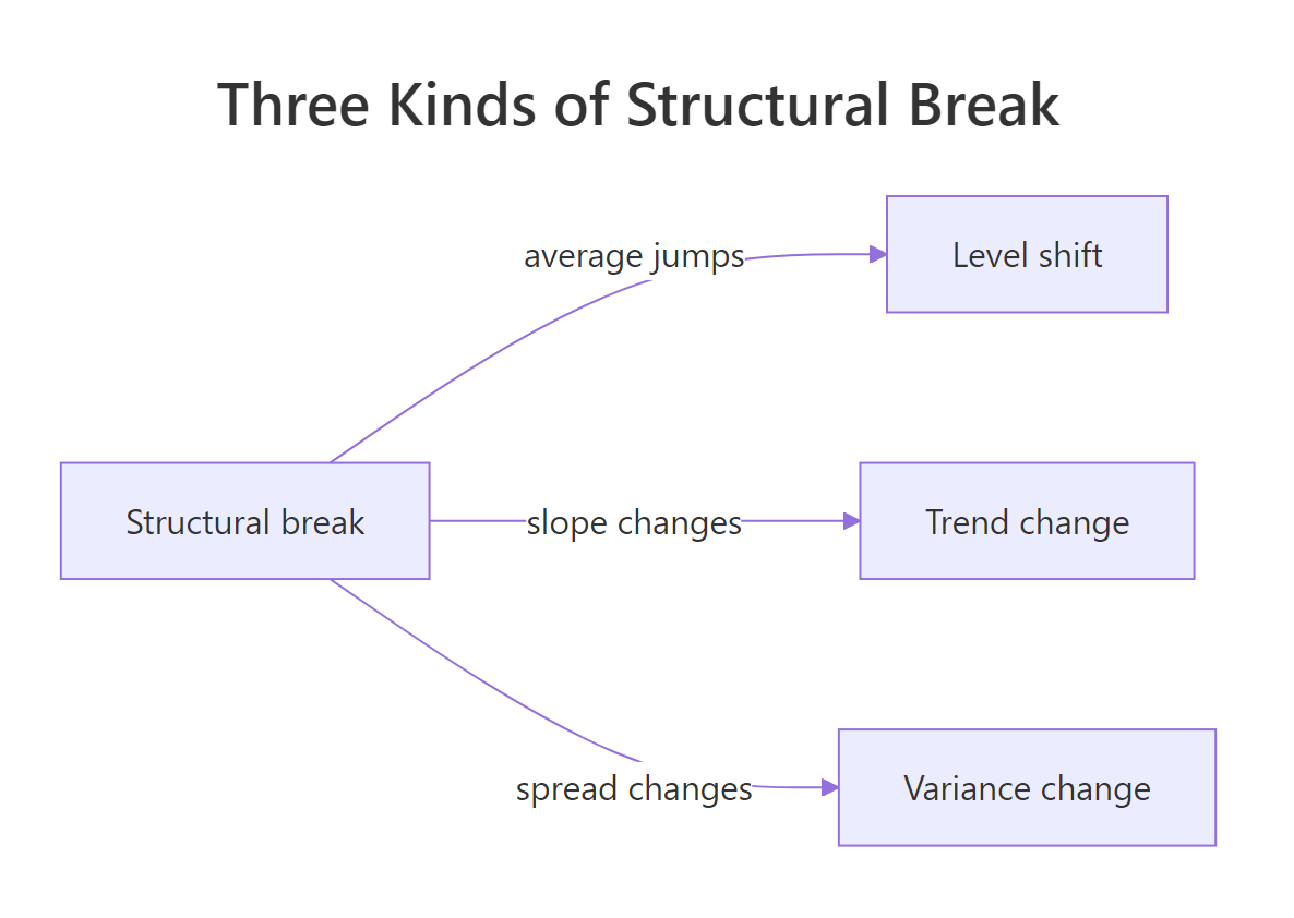
Figure 1: The three kinds of structural break a forecaster must handle.
A break can move the level (the average jumps, like our sales), bend the trend (steady growth suddenly plateaus), or widen the variance (the series becomes noisier without changing its average). Our example is a level shift, the most common and the easiest to see. Now watch what a standard forecast does with it. We hold out the last 12 months as a test set, then forecast them using the simplest baseline there is: the average of all history.
Look at the forecast line in the plot: it sits at roughly 116, floating in empty space between the old regime and the new one. The red line of reality is up near 150, far above it. On the test set the error is large, a root mean squared error (RMSE, the typical size of a forecast miss) of 32.72 units. The forecast is bad not because the method is broken, but because it averaged the 72 pre-break months near "100" with the 36 post-break months near "150" in the training window and landed at a number that describes neither.
That is the mistake this whole tutorial exists to prevent. But before you can forecast through a break, you have to know where it is. So the first job is detection.
Try it: Rebuild the series with a bigger jump, from 100 up to 190, keep the same 108-month training window, and forecast it with meanf(). Read off the single point forecast and notice how it again lands between the two levels.
Click to reveal solution
Explanation: The training window holds 72 months near 100 and 36 months near 190, so their average is about 130.8, a forecast stranded halfway between the two regimes. A larger break just makes the averaging error larger.
How do you find where the break happened?
To forecast through a break you first have to locate it. "Eyeballing the chart" does not scale to hundreds of series and misses breaks that are real but subtle. Instead we let an algorithm scan the series and find the split point that best explains the data. The changepoint package does exactly this, and it runs directly in your browser here.
The core idea is simple. For every possible split point, the algorithm measures how much better the data is described by two segments (each with its own average and spread) instead of one. The split that gives the biggest improvement, after paying a penalty for added complexity, is the break. We use cpt.meanvar(), which allows both the mean and the variance to change across the break.
The function found the break at month 72, exactly where we planted it. The cpts() helper returns the break location, and param.est() reports what each segment looks like: the average is 99.2 before the break and 149.7 after, matching the true regimes. The method = "PELT" argument names the search algorithm (Pruned Exact Linear Time), which finds the optimal split points quickly even on long series. In one call, you have turned "something changed around here" into a precise month.
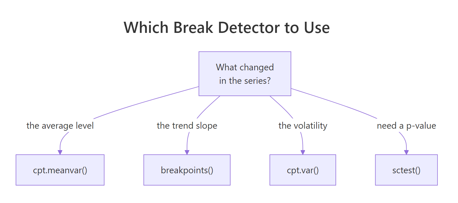
Figure 2: Match the detector to the kind of change you expect.
There is one trap worth naming, because it bites almost everyone the first time. The sister function cpt.mean() searches for shifts in the average while assuming the noise level is fixed and equal to one. Real data rarely obeys that, so it tends to chop the series into dozens of tiny false segments. Using cpt.meanvar(), which estimates the noise as it goes, avoids the problem and finds the single true break.
The same package detects breaks in variance, where the average holds steady but the series suddenly gets noisier. That matters for forecasting because it inflates your prediction intervals, not your point forecast. Here we build a series whose spread jumps at observation 80 and let cpt.var() find it.
The detector placed the variance break at observation 82 (the truth was 80) and estimated the spread as 3.3 in the calm first half against 66.1 in the turbulent second half. The average never moved, but the spread around it jumped sharply. Which detector you reach for depends on what kind of change you expect, and Figure 2 above is your cheat sheet.
Try it: The series below has two clear halves. Run cpt.meanvar() on it and read the break location with cpts().
Click to reveal solution
Explanation: The series switches from an average of 5 to an average of 12 at observation 50, and cpt.meanvar() with method = "AMOC" returns that single split point.
How do the classic tests confirm a structural break?
The changepoint approach answers "where is the break?" A second family, from econometrics, answers a slightly different question: "is there a break at all, and can I put a confidence interval and a p-value on it?" That family lives in the strucchange package. It is built on regression, so it also handles breaks in a trend, not just a level. These functions need a full R installation rather than the in-browser engine, so the blocks below are marked to run locally, but every result is real.
The workhorse is breakpoints(). We regress the series on a constant (sales ~ 1), which tells the function to look for shifts in the average, and it returns the split that minimises the total squared error, along with a confidence interval.
library(strucchange)

bp <- breakpoints(sales ~ 1)
bp$breakpoints
#> [1] 72
confint(bp)
#>   2.5 % breakpoints 97.5 %
#> 1    71          72     73
The estimate agrees with changepoint to the month: the break is at observation 72, and the 95% confidence interval is a tight window of months 71 to 73. That interval is genuinely useful, it tells you how sure you can be about the timing, which a point estimate alone never does. Regressing on sales ~ trend instead would hunt for a change in slope, the tool for a trend break, and the Bayesian Information Criterion picks how many breaks the data actually supports.
Sometimes you need a formal yes-or-no answer before you act. Two classic tests provide it. The supF test (also called the Quandt Likelihood Ratio) scans every candidate break date and reports the largest instability it finds, while the OLS-CUSUM test tracks the running sum of forecast errors and flags when it drifts too far from zero.
qlr <- Fstats(sales ~ 1)
sctest(qlr)
#> 	supF test
#> data:  qlr
#> sup.F = 1962.8, p-value < 2.2e-16

ocus <- efp(sales ~ 1, type = "OLS-CUSUM")
sctest(ocus)
#> 	OLS-based CUSUM test
#> data:  ocus
#> S0 = 5.1904, p-value < 2.2e-16
Both tests return a p-value below 2.2e-16, far under any sensible threshold, so both reject the idea that the series is stable. The huge supF statistic of 1962.8 is the strength of the single most significant break; the CUSUM statistic of 5.19 confirms the running errors wander far from zero. In plain terms: yes, there is definitely a break, and you are safe to treat the series as two regimes.
Try it (run locally): The bp object above stores the break index in bp$breakpoints. Convert that index into a calendar year and month, remembering the series starts in January 2016.
# your code here: read bp$breakpoints, then compute the year and month.
# Hint: year = 2016 + (index - 1) %/% 12, month = (index - 1) %% 12 + 1
Click to reveal solution
brk_index <- bp$breakpoints
c(index = brk_index,
  year  = 2016 + (brk_index - 1) %/% 12,
  month = (brk_index - 1) %% 12 + 1)
#> index  year month
#>    72  2021    12
Explanation: Month 72 of a series that starts in January 2016 is December 2021, so the last stable month is December 2021 and the new regime begins in January 2022.
How do you forecast through a structural break?
Now for the payoff. You have found the break; the question is how to forecast the future without letting the pre-break past pollute it. There are three practical strategies, and Figure 3 lays them out. Each one takes the detected break and turns it into a reliable forecast; they differ in how much data they keep and how much modelling they do.
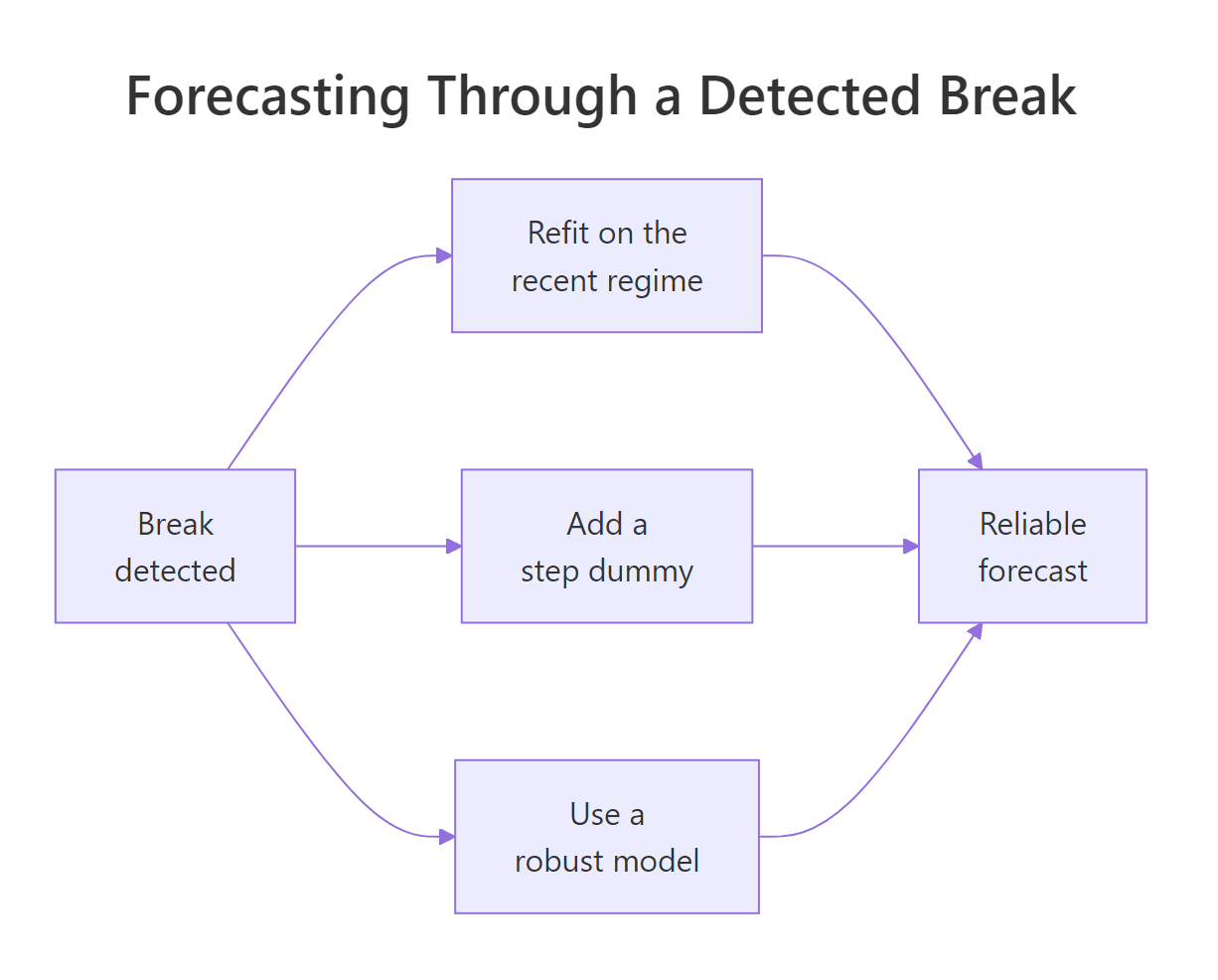
Figure 3: Three routes from a detected break to a reliable forecast.
Strategy 1: refit on the recent regime. The simplest fix is also the most effective: detect the break, throw away everything before it, and fit your model on the current regime only. We detect the break inside the training data, keep the post-break months, and forecast from there.
The test-set RMSE drops from 32.72 with the full history to 6.72 on the recent regime, a nearly fivefold improvement, from the exact same forecasting method. All we changed was the data we fed it. By fitting only the post-break months, the average settles at the true new level of about 150 instead of being dragged down by ancient history.
Strategy 2: model the break with a step dummy. Refitting throws data away, which stings when the post-break regime is short. A thriftier option keeps every observation but tells the model exactly when the level shifted, using a step variable that is 0 before the break and 1 after. We add it as an external regressor to an ARIMA model.
The model reads the break perfectly. It estimates a baseline level of 99.2 and a step coefficient of 51.0, which recovers the true jump of about 50 units almost exactly. The test RMSE matches the refit approach at 6.72, but notice the training RMSE is lower (6.00 versus 6.87), because this model learned from all 108 months instead of just the recent 36. What that step regressor does is captured in one small equation.
$$y_t = \beta_0 + \beta_1 D_t + \varepsilon_t$$
Where:
- $y_t$ = the observed value at time $t$
- $\beta_0$ = the baseline level before the break
- $D_t$ = the step dummy, equal to 0 before the break and 1 after
- $\beta_1$ = the size of the level shift (here about 51)
- $\varepsilon_t$ = the remaining noise
If you are not interested in the algebra, skip it: the code already showed that $\beta_1$ lands on the true shift. To forecast, you simply set the dummy to 1 for every future month, since the future lives in the post-break world.
Strategy 3: prefer break-robust models and watch your intervals. Some models absorb a level shift better than others. An adaptive model like exponential smoothing (ETS) keeps re-estimating the current level, so after a jump it quickly re-anchors and its point forecast survives. The hidden cost is the prediction interval: the break inflates the model's estimate of the noise, so its intervals balloon. Compare the same model fit on all history versus the recent regime.
The point forecasts are close (RMSE 7.79 versus 6.72), confirming that ETS re-anchored to the new level on its own. But the 95% prediction interval is 36.2 units wide on the full history and only 27.7 units wide on the clean regime. The break inflated the full-history model's estimate of the noise, so its intervals are wider than the recent regime warrants. For a trend break rather than a level shift, the robust choice is a damped trend, which stops the model extrapolating a slope that no longer holds.
Try it: Fit an ETS model on the post-break window post and read its test-set RMSE, confirming it matches the refit result.
Click to reveal solution
Explanation: Fitting ETS on the clean post-break regime gives a test RMSE of 6.72, the same as the naive refit, because once the old regime is gone there is little left to model beyond the new level.
Which detector and forecasting strategy should you pick?
You now have a toolbox. The trick is matching the tool to the break. The table below is the decision guide: identify the kind of change, pick the detector, then pick the forecasting move.
| Break is in the | Looks like | Detect with | Forecast with |
|---|---|---|---|
| Level | The average jumps to a new plateau | cpt.meanvar() or breakpoints(y ~ 1) | Refit on the regime, or a step dummy |
| Trend | Growth speeds up, slows, or reverses | breakpoints(y ~ trend) | Refit, or a damped trend |
| Variance | Same average, suddenly noisier | cpt.var() | Keep the model, widen the intervals |
To make this repeatable, wrap the common case in a tiny helper. It runs the single-break detector, returns the break month, and reports the average in each regime so you can see the size of the shift at a glance.
The helper reports the break at month 72 and the two regime averages, 99.2 and 149.7. With the shift size in hand (about 50 units on a base of 100, a big move), you would confidently refit on the recent regime. A tiny shift, by contrast, might not be worth acting on at all, which is the judgement the next callout is about.
Try it: Run the diagnose_break() helper on the mystery series below, read the break location and the two regime averages, and decide which forecasting strategy fits.
Click to reveal solution
Explanation: The helper finds a break at observation 40 with the average moving from 30.2 to 54.8, a large level shift, so refitting on the post-break regime (or a step dummy) is the right call.
Complete Example: forecasting website traffic after a launch
Let's put every piece together on a fresh, realistic problem. A website runs steady at about 1,200 daily sessions, then a marketing launch on day 60 lifts it permanently to around 1,750. We have 180 days of history and want to forecast the next three weeks. First we detect the break.
The detector pins the break to day 59, one day before the true launch, and estimates the two levels as 1,221 and 1,758 sessions, both spot on. Now we forecast the final 21 days three ways: with the full history, with a refit on the post-break regime, and with a step dummy, then compare their errors on the held-out test set.
The verdict is stark. The full-history forecast misses by an RMSE of 215.3 sessions, because it averages the quiet pre-launch weeks with the busy post-launch ones. Both break-aware strategies cut that error to 83.2, more than a twofold improvement, by forecasting from the world that actually exists now. This is the entire workflow in miniature: detect the break, then either refit on the recent regime or model the break explicitly, and never let stale history set your baseline.
Practice Exercises
These two exercises combine detection and forecasting. Each uses its own variables so nothing clashes with the tutorial code above, and every expected number is shown so you can check your work.
Exercise 1: Detect a break and beat the full-history forecast
A series of 96 months holds at an average of 40 until month 60, then jumps to 65. Detect the break in the first 84 months, refit meanf() on the post-break regime, and compare its test-set RMSE (on the last 12 months) against a full-history forecast. You should find the refit forecast is dramatically better.
Click to reveal solution
Explanation: The detector finds the break at month 60. Refitting on the post-break regime cuts the test RMSE from 17.21 to 4.84, because the forecast now sits at the true new level of 65 instead of averaging in the old level of 40.
Exercise 2: Recover the size of a level shift with a step dummy
A series of 100 observations shifts up by 15 units at observation 51. Without discarding any data, fit an ARIMA model with a step dummy, recover the estimated shift from the coefficients, and forecast 12 steps ahead. The step coefficient should land near 15 and the forecast near 35.
Click to reveal solution
Explanation: The model estimates a baseline of 19.9 and a step of 14.5, recovering the true shift of 15 without throwing away a single observation. Setting the dummy to 1 for the future gives a forecast of 34.4, right at the new regime level.
Frequently Asked Questions
What is the difference between a structural break and an outlier? An outlier is a single unusual point that the series returns from immediately. A structural break is a permanent change in the rule generating the data: after it, the new behaviour continues. Detect outliers with spike-focused methods; treat breaks by re-scoping your training data or modelling the shift.
How much post-break data do I need before I can trust a refit? Enough to estimate your model. A plain level model needs only a handful of points, while a seasonal model needs at least a full cycle or two. If the post-break regime is too short, keep the full sample and use a step dummy instead of refitting.
Can I just forecast without detecting the break? Sometimes. Adaptive models such as ETS and differenced ARIMA partly absorb a level shift on their own, so the point forecast may survive. But they inflate their prediction intervals and mishandle trend breaks, so explicit detection plus a refit or step dummy is safer and more accurate.
Does differencing or auto.arima fix structural breaks automatically? Only partly. Differencing turns a one-time level shift into a single spike in the differenced series, which localises the damage but does not remove it, and it does nothing for a trend or variance break. Detecting the break and acting on it is more reliable than hoping the model absorbs it on its own.
changepoint or strucchange, which should I use? Use changepoint for fast, general detection of shifts in mean or variance, especially across many series. Use strucchange when you want confidence intervals, a formal significance test, or detection of a break in a regression relationship such as a trend. They usually agree on the location.
Summary
Structural breaks are the reason a perfectly reasonable forecast can be badly wrong: the model is describing a past that no longer applies. The fix is a two-step discipline, detect the break, then forecast from the current regime.
| Concept | Tool in R | Takeaway |
|---|---|---|
| See the break | plot() plus regime means | A level shift, trend bend, or variance jump splits history into regimes |
| Locate the break | cpt.meanvar(), cpt.var() | changepoint pins the break month in one call, in your browser |
| Confirm the break | breakpoints(), sctest() | strucchange adds confidence intervals and a formal p-value |
| Refit on the regime | window() plus meanf()/ets() | Dropping pre-break data cut our RMSE nearly fivefold |
| Model the break | Arima(xreg = step) | A step dummy keeps all data and recovers the shift size |
| Robust forecasting | ets(), damped trend | Adaptive models survive the point forecast but widen their intervals |
The through-line: never let data from before a break set your baseline. Detect it, then either refit on the recent regime or tell the model exactly when the world changed.
References
- Killick, R. & Eckley, I. A. - changepoint: An R Package for Changepoint Analysis. Journal of Statistical Software, 58(3), 2014. Link
- Zeileis, A., Leisch, F., Hornik, K. & Kleiber, C. - strucchange: Testing for Structural Change in Linear Regression Models. Journal of Statistical Software, 7(2), 2002. Link
- Hyndman, R. J. & Athanasopoulos, G. - Forecasting: Principles and Practice, 3rd edition. OTexts, 2021. Link
- changepoint package reference. Comprehensive R Archive Network. Link
- strucchange package reference. Comprehensive R Archive Network. Link
- strucchange reference manual (PDF). Comprehensive R Archive Network. Link
- Hyndman, R. J. - forecast: Arima() function reference. Link
Continue Learning
- Choosing a Forecasting Model in R - how to compare competing forecasts on a hold-out set, the exact method used to grade our three strategies.
- Measuring an Intervention's Effect with CausalImpact in R - when the break is a known event you caused, estimate how big its effect really was.
- Forecasting Very Short (and Very Long) Time Series in R - the recent-window idea behind refitting on a regime, generalised to any long series.