Forecasting Very Short (and Very Long) Time Series in R
The length of a time series decides which forecasting methods are safe to use. Too few observations and you cannot estimate a model reliably. Too many and a single fixed model quietly averages over dynamics that have long since changed. This tutorial shows you how to handle both extremes in R.
Why does the length of a time series change how you forecast it?
Most forecasting tutorials hand you a tidy series with a couple of hundred observations and a clean seasonal pattern. Real projects are rarely that kind. Sometimes you have a brand-new product with twelve months of sales, and sometimes you have three decades of daily readings. The forecasting recipe is different at each extreme, and getting it wrong is a common, silent mistake.
Here is a reassuring fact to start with: you can forecast a series with only twelve points. Let's prove it. We load the forecast package, create a short series of monthly signups, and let R pick and fit a model automatically.
That worked. The auto.arima() function found a model, and forecast() produced three point forecasts (the "Point Forecast" column) plus 80% and 95% prediction intervals. The forecasts continue the upward trend, climbing from 97 to about 107 at the first step and on to 126 by the third. Twelve points were enough to see a trend and extend it.
So if twelve points can be forecast, what actually goes wrong at the extremes? Two different things, pulling in opposite directions.
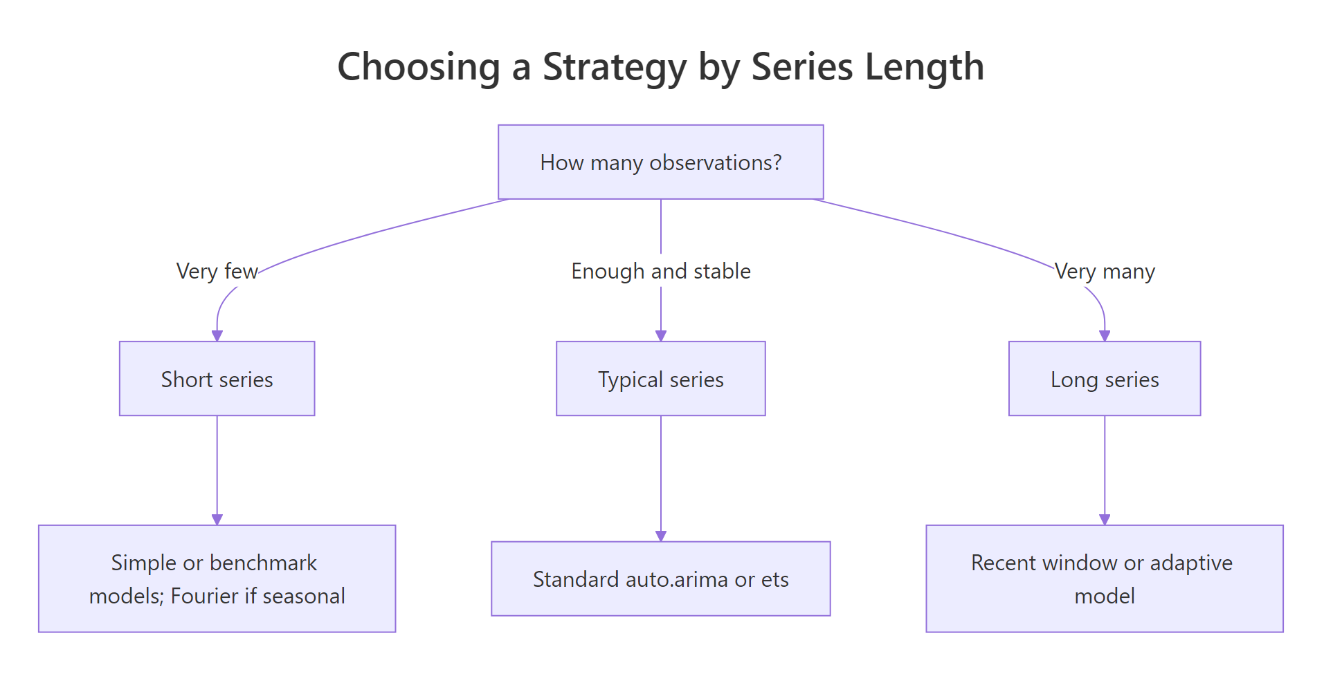
Figure 1: Series length points you to a forecasting strategy.
With a very short series, the danger is on the supply side: there is not enough information to estimate anything complicated, so you must keep the model tiny. With a very long series, the danger is subtler: there is so much history that a single model has to fit patterns from long ago that no longer hold today.
How many observations do you need to fit a forecasting model?
Before we can talk about "too few" observations, we need to know what "few" means. The honest answer is refreshingly simple. You can only estimate a model when you have more data points than the number of quantities the model has to learn from the data.
$$n > k$$
Here $n$ is the number of observations and $k$ is the number of parameters the model estimates. Every parameter is a number the fitting procedure has to pin down, and each one needs data to support it. Let's see how many parameters our signups model actually used.
Read the second line of that output: ARIMA(1,2,0). Those three numbers are the orders of the model. For a non-seasonal ARIMA written as $\text{ARIMA}(p,d,q)$, the number of estimated parameters is
$$k = p + q + P + Q + (\text{1 if a constant, mean, or drift is included})$$
where $P$ and $Q$ are the seasonal orders (zero here, because this series has no season). The middle number, $d = 2$, is differencing: it transforms the data before fitting and costs no estimated parameters. So this model has $p = 1$ autoregressive term and nothing else, which is exactly the [1] 1 that length(coef()) reports. One parameter, twelve observations. Comfortably within budget.
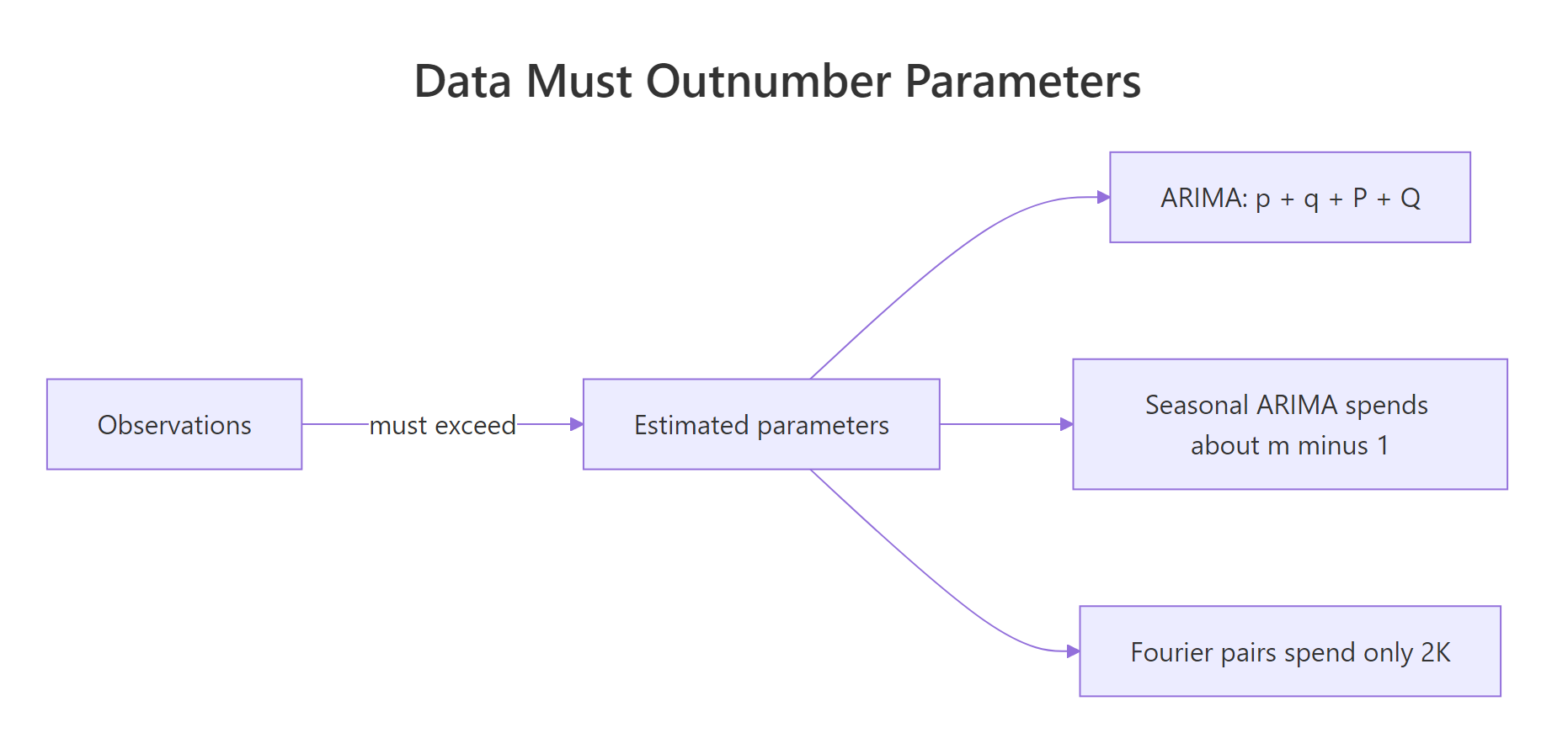
Figure 2: You need more observations than the parameters your model estimates.
You may have heard that ARIMA needs "at least 30 observations." That rule is a myth. It ignores both the number of parameters and how noisy the data is, and it has no basis in theory or practice. What happens instead is that the automatic search simply refuses to estimate parameters it cannot support. Watch what auto.arima() does with ten noisy points that have no clear trend.
The chosen model is ARIMA(0,0,0) with non-zero mean: no autoregression, no differencing, no moving average, just an estimate of the average level. With ten scattered points and no real signal, the safest forecast is the mean, which is exactly what the search returns. This is the myth-busting rule of thumb in action: the model gets as simple as the data demands.
Try it: Fit a model to the built-in uspop series (US population, 19 observations) with auto.arima(), then count its parameters. How few does it use?
Click to reveal solution
Explanation: The model is ARIMA(0,2,0), a pure "second difference" random walk. It estimates zero coefficients: it simply projects the recent local trend forward. Even 19 smooth points need no estimated parameters, which is the shortest budget possible.
How do you forecast a very short series?
When data is scarce, your best friends are the simplest possible models. A forecasting benchmark is a rock-bottom method you can always fall back on, and there are three you should know. The mean method forecasts every future value as the average of the past. The naive method forecasts the last observed value. The drift method extends the straight line drawn between the first and last observations.
Let's run all three on the signups trend and compare.
Look at how differently they behave. The mean method predicts a flat 53.4, which is nonsense for a series that has been climbing steadily. The naive method predicts a flat 97, the last value, ignoring the trend. Only the drift method captures the upward slope, forecasting 104, 111, then 118. And notice how close those drift numbers are to the automatic model's forecasts from earlier, which climbed from about 107 to 126. When a simple benchmark and a fancier model nearly agree, that agreement is a signal you can trust the result.
Benchmarks matter even more when you cannot hold out a test set. With a short series there simply are not enough points to split off a chunk for evaluation. The trick is a model-selection score called the AICc, which R prints in every model summary. You can think of the AICc as a stand-in for one-step out-of-sample error: it rewards a good fit while penalizing extra parameters, so a lower AICc points to a model that should forecast well without over-fitting. That is why auto.arima() and ets() lean on it to pick simple models when data is thin.
Try it: Produce a drift forecast for the noisy annual_sales series, three steps ahead. Because that series has no real trend, the drift forecast should barely move.
Click to reveal solution
Explanation: The average change across annual_sales is tiny, so the drift line is almost flat. The forecast nudges up by less than one unit per step, which is appropriate for a series with no clear direction.
What if the short series is also seasonal?
Seasonality raises the stakes for short data, because a seasonal model is expensive. To learn a monthly pattern, a seasonal model has to estimate a separate behavior for each month, which spends roughly $m - 1$ parameters, where $m$ is the number of periods per cycle ($m = 12$ for monthly data). With only two years of monthly data, you barely have enough points to see each month twice, let alone estimate a full seasonal model on top of a trend.
Let's watch this happen. We take the first two years of the classic AirPassengers series, 24 monthly observations, and let auto.arima() decide.
Notice what is missing. The chosen model is ARIMA(0,0,2) with no seasonal part at all. The search decided that 24 points could not support a seasonal model, so it dropped seasonality entirely. That decision has consequences for the forecast.
The forecast wobbles for two months and then flatlines at 134.2, the series mean. A traveler could tell you air traffic peaks every summer, but this model has thrown that knowledge away. We need a cheaper way to represent the season.
That cheaper way is Fourier terms. Instead of estimating a separate value for every month, we approximate the seasonal shape with a few smooth sine and cosine waves. Each pair of waves is one "Fourier term" of order $K$, and $K$ pairs cost only $2K$ parameters. Choose a small $K$ and you capture the seasonal shape for a fraction of the parameter budget a full seasonal model would demand. We add these terms as an external regressor and turn the built-in seasonal search off.
The model is now a regression with ARIMA errors. The S1-12 and C1-12 coefficients are the sine and cosine of the first Fourier pair, and they encode the seasonal shape using just two numbers. Now forecast with matching Fourier terms for the next twelve months.
This forecast follows the season. It dips in the winter months, rises to a summer peak around July at 149.4, and falls again toward year end, the seasonal pattern the earlier flat forecast could not represent. We recovered the season with only two extra parameters instead of eleven.
Try it: Build Fourier terms of order K = 2 for air_short and look at the first three rows. You should see four columns, two sine-cosine pairs.
Click to reveal solution
Explanation: With K = 2 you get four columns: the first sine-cosine pair (S1-12, C1-12) and a second, faster pair (S2-12, C2-12). More pairs let the seasonal curve bend more sharply, at the cost of two extra parameters each.
Why do forecasts get worse when a series is very long?
Now flip to the other extreme. It seems obvious that more data should always help, and for short and medium series it usually does. But a long series hides a trap. Real data does not actually come from the neat model we fit to it. For a couple of hundred observations, the model is a fine approximation. Stretch to thousands of points spanning many years, and the gap between the real process and the model becomes impossible to ignore, because the world that generated the early data is not the world that generated the recent data.
A single fixed model has to fit the entire history at once. If the trend was steep for decades and then flattened, the model splits the difference and gets the present wrong. Let's manufacture exactly that situation: 480 observations that climb steadily and then level off near the end, and fit one model to all but the last two years.
We held out the final 24 points as test so we can grade the forecast honestly. The model fitted to the full history is an ARIMA(1,1,1). Now compare its forecast to what really happened over that held-out window.
The forecast keeps rising, reaching 316.3 by the end, while the actual series had already flattened and sat at 305.4. The model learned the long, steep climb that dominated most of its history and projected it forward, blind to the recent change in behavior. The extra decades of data actively hurt the forecast.
How do you forecast a very long series?
The simplest fix follows directly from the diagnosis. If you only care about forecasting the next few points, throw away the ancient history and fit the model to a recent window. This is equivalent to letting the model change over time, and it is far easier to reason about. Let's refit the very same method to just the last 72 observations of the training data.
Same function, same automatic search, just less history. Now let's grade both forecasts against the held-out test window using root mean squared error, where smaller is better.
The recent window nearly triples the accuracy, cutting the error from 6.57 to 2.36. By ignoring the era that no longer applies, the shorter fit matched the current, flatter behavior. This is the counterintuitive heart of long-series forecasting: sometimes the best thing to do with old data is to discard it.
There are gentler alternatives to a hard cutoff. Models that already adapt to local behavior, like exponential smoothing or a differenced ARIMA, put more weight on recent observations and cope better with slow change than a rigid regression would. And if the seasonality is long or complex, dynamic harmonic regression (an ARIMA model with Fourier terms) scales to it without exploding the parameter count.
Try it: Fit auto.arima() to the last 120 observations of train and report the chosen model order with arimaorder().
Click to reveal solution
Explanation: A different window can lead the automatic search to a different model, here an ARIMA(0,2,2). That is expected: each window sees a slightly different slice of behavior, which is exactly why the window size is a choice worth testing rather than fixing blindly.
Complete Example: a length-aware forecasting workflow
Let's tie the whole tutorial into one reusable helper. Given any time series, it reports how much data you have, whether it is seasonal, and which strategy to reach for first. Think of it as a triage step you run before modeling.
Now run it across the four series we have met, from the twelve-point trend to the 480-point simulation.
Each series lands in the right bucket. The thresholds here (fewer than 24 points, or fewer than three full seasonal cycles, or more than 400 points) are deliberately rough. They are a starting point for the decision, not a law. The one non-negotiable rule, which the myth of "30 observations" ignored, is to confirm your choice out-of-sample whenever you possibly can.
Practice Exercises
These combine several ideas from the tutorial. Try each one before opening the solution.
Exercise 1: Trust-check a short forecast with a benchmark
Forecast the signups series four steps ahead two ways: once with auto.arima() and once with the drift method. Put the two forecasts side by side in a data frame so you can see whether they agree. Close agreement is your evidence that the automatic model is trustworthy on this short series.
Click to reveal solution
Explanation: The automatic model and the drift benchmark track each other closely, drifting apart by only a handful of units at the four-step horizon. When a bare-bones benchmark shadows your model this tightly, you can forecast the short series with confidence.
Exercise 2: Find a good window for the long series
For the long series, the full history was a poor teacher. Write a function that fits auto.arima() to the last k observations of train, forecasts 24 steps, and returns the RMSE against test. Run it for windows of 48, 72, 120 and 240, then compare. Is the shortest window always best?
Click to reveal solution
Explanation: Every recent window beats the full-history RMSE of 6.57, which confirms the core lesson. But the best window here is 120, not the shortest, and the numbers are not perfectly ordered. Window size is a genuine tuning knob: test a few, do not assume smaller is automatically better.
Frequently Asked Questions
Is 30 the minimum number of observations for an ARIMA model?
No. There is no theoretical or practical basis for the "30 observations" rule. The only firm requirement is that you have more observations than parameters, and the automatic search will pick a model simple enough to satisfy that. In practice you want comfortably more than the bare minimum, but the exact number depends on how noisy your series is, not on a magic constant.
What is the absolute fewest points I can forecast?
You can produce a forecast from a handful of points, because benchmarks like the naive and drift methods estimate zero or one parameter. Whether that forecast is any good is a separate question. With very few points, prefer a benchmark and treat the forecast as a rough guide rather than a precise prediction.
Why did auto.arima() ignore the seasonality in my data?
Because your series was probably too short to support a seasonal model. A seasonal model needs to see each season repeated several times, spending about $m - 1$ parameters on the pattern. When there are not enough cycles, the search drops the seasonal part. Add Fourier terms with a small K to represent the season cheaply instead.
Should I always forecast a long series from its most recent window?
Not blindly. A recent window helps when the dynamics have shifted over time, which is common for long real-world series. If the process has genuinely been stable for decades, the full history can help. The safe move is to test both against a held-out window and let accuracy decide, as Exercise 2 shows.
Does adding more historical data always improve a forecast?
No. More data helps up to a point, then can hurt if the older data was generated by a different regime. A single model fitted to a very long series averages across all those regimes and may forecast the present poorly. Beyond a few hundred observations, check whether a recent window or an adaptive model does better.
Summary
The length of your series is the first thing to check before you forecast, because it dictates what is even possible. Short series force simplicity; long series reward forgetting.
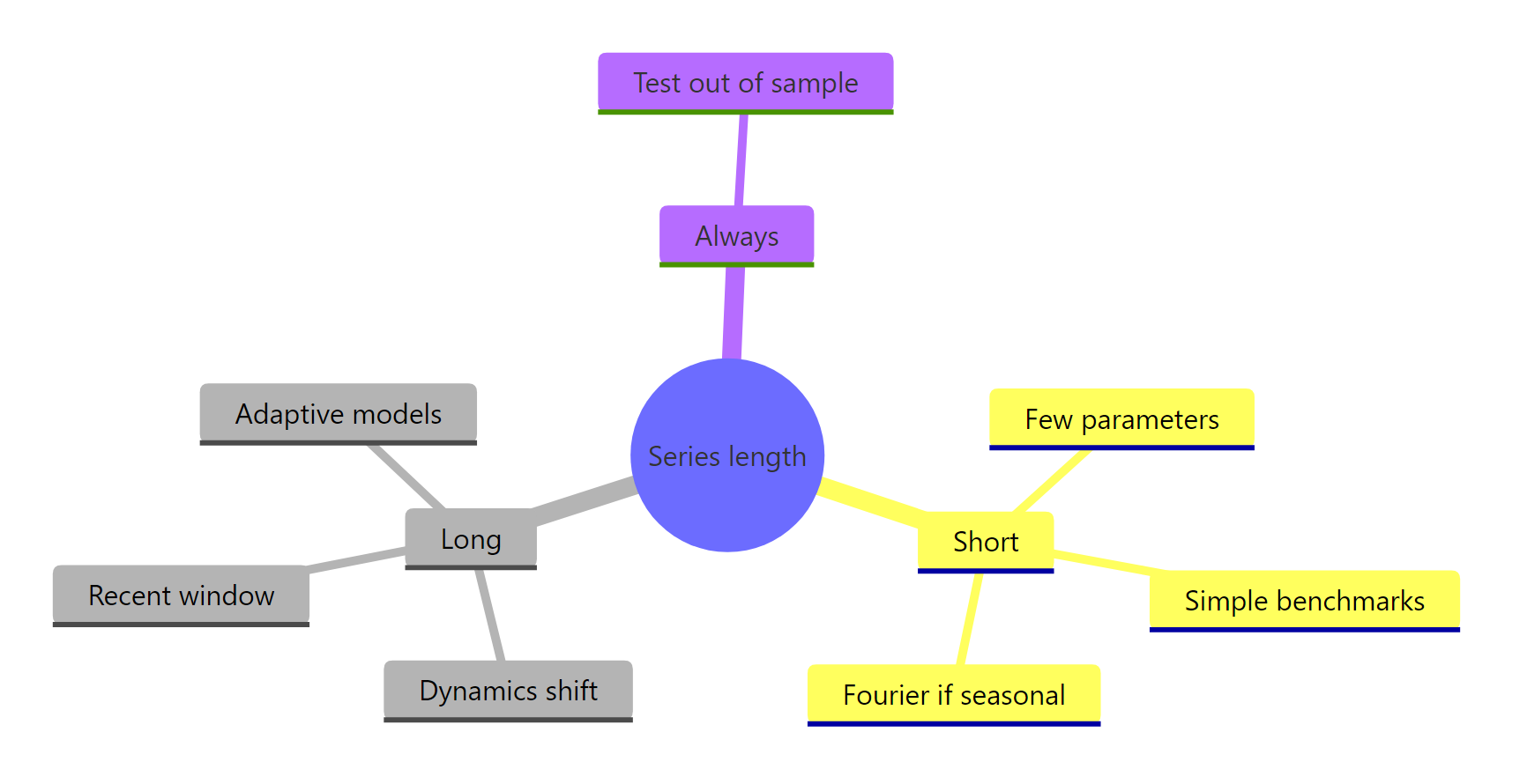
Figure 3: The short-versus-long decisions at a glance.
| Situation | The risk | What to do in R |
|---|---|---|
| Very short, non-seasonal | Too few points to estimate anything complex | Let auto.arima() or ets() pick a low-parameter model; compare to naive() and rwf(drift = TRUE) |
| Very short, seasonal | A seasonal model spends too many parameters | Add fourier() terms with a small K and set seasonal = FALSE |
| Typical length | Few special concerns | Standard auto.arima() or ets() |
| Very long | One model averages over changed dynamics | Fit a recent window, or use adaptive models; validate window size out-of-sample |
The single rule that survives every case is the one the "30 observations" myth forgot: keep your model no more complex than your data can support, and confirm the choice out-of-sample whenever you can.
References
- Hyndman, R.J. - Fitting models to short time series. Link
- Hyndman, R.J. - Fitting models to long time series. Link
- Hyndman, R.J. & Athanasopoulos, G. - Forecasting: Principles and Practice, Section 12.7: Very long and very short time series. Link
- Hyndman, R.J. & Athanasopoulos, G. - Forecasting: Principles and Practice (3rd ed.), Dynamic harmonic regression. Link
- Hyndman, R.J. & Khandakar, Y. - Automatic Time Series Forecasting: The forecast Package for R. Journal of Statistical Software (2008). Link
- forecast package reference -
fourier(). Link - Hyndman, R.J. & Athanasopoulos, G. - Forecasting: Principles and Practice (3rd ed.), full text. Link
Continue Learning
- auto.arima() in R - how the automatic search chooses ARIMA orders, the engine behind most of this tutorial.
- Forecast Accuracy in R - RMSE, MAE, and how to score forecasts properly on a holdout.
- ETS Models in R - exponential smoothing, the adaptive model family that copes well with slowly changing long series.